Detector de pontos de interesse baseado em características visuais e de profundidade

DETECTOR DE PONTOS DE INTERESSE BASEADO

EM CARACTERÍSTICAS VISUAIS E DE

LEVI OSTERNO VASCONCELOS

DETECTOR DE PONTOS DE INTERESSE BASEADO

EM CARACTERÍSTICAS VISUAIS E DE

PROFUNDIDADE

Dissertação apresentada ao Programa de Pós--Graduação em Ciência da Computação do Instituto de Ciências Exatas da Universidade Federal de Minas Gerais como requisito par-cial para a obtenção do grau de Mestre em Ciência da Computação.

O

: E

R

N

C

: M

F

M

C

Belo Horizonte

LEVI OSTERNO VASCONCELOS

A KEYPOINT DETECTOR BASED ON VISUAL AND

DEPTH FEATURES.

Dissertation presented to the Graduate Pro-gram in Ciência da Computação of the Uni-versidade Federal de Minas Gerais in partial fulfillment of the requirements for the degree of Master in Ciência da Computação.

A

: E

R

N

C

-A

: M

F

M

C

Belo Horizonte

c

2015, Levi Osterno Vasconcelos.

Todos os direitos reservados.

Vasconcelos, Levi Osterno

V278d Detector de pontos de interesse baseado em

características visuais e de profundidade / Levi Osterno Vasconcelos. — Belo Horizonte, 2015

xx, 49 f. : il. ; 29cm

Dissertação (mestrado) — Universidade Federal de Minas Gerais

Orientador: Erickson Rangel do Nascimento

Coorientador: Mario Fernando Montenegro Campos

1. Computação - Teses. 2. Visão por computador. 3. RGB-D, 4. Keypoints. I. Orientador. II. Coorientador. III Título.

Acknowledgments

I am truly thankful for everyone who helped me, directly and indirectly, towards the

conclu-sion of this work.

First, I would like to thank my family; my parents José Sidney and Carmen Angela. My brother Jansen and my sister Tainá and last, but not least, my wife Rebeca for all the

given support during the whole process. For you all, my sincere gratitude and love.

To my advisors Erickson Rangel do Nascimento and Mario Fernando Montenegro

Campos (Co-orientation), I would like to register my admiration and sincere gratitude for

all the lessons, orientation and knowledge that were directed towards me. It was a great and

huge experience of self-improvement and learning. Thank you.

Also, the amazing laboratory that has built an incredible community, I would like to

thank the VeRLab crew: Paulo Drews, Elerson Rubens, Jhielson Pimentel, Omar Pino, David

Saldana, Hector Azpurua, Daniel Balbino, Rafael Colares, Ramon Melo, Samuel Servulo, Igor Campos, Vinicius Santos, Claudio Fernandes and many others that i am forgetting and,

for sure, a will be ashamed of once I remember.

For my personal friends, for all the support and fun we had during the whole process:

Rogerio Fonteles, Samuel Servulo, Vladimir Portela, Paulo Drews, Igor Campos, Omar Pino,

Elerson Rubens, Jhielson Pimentel, Clayson Celes, Caio Rodrigues, Gustavo Malkomes,

Rodrigo Viana.

For the financial and infra-structure support, my sincere thanks for CNPQ, VeRLab

and UFMG.

Resumo

Em sistemas de visão computacional, é prática comum representar partes de imagens por um

conjunto de pontos cuidadosamente selecionados, tais pontos são identificados de acordo

com características convenientes à aplicação. Exemplos de características são: arestas,

quinas,blobseridges. Tais regiões são denominadas comopontos de interesseoukeypoints.

Inúmeras aplicações em visão computacional necessitam da extração de pontos de

in-teresse. Apesar da grande quantidade de trabalhos presentes na literatura de detectores de

pontos de interesse em imagens, poucas metodologias combinam, de forma eficiente,

infor-mações visuais e geométricas.

Neste trabalho, apresentamosKeypoints from Visual and Depth Data(KVD), um novo

detector de pontos de interesse invariante a escala que combina informação de textura e

ge-ometria utilizando operações de baixo custo e uma árvore de decisão. Também apresentamos

a análise de duas abordagens para a fusão de informação para dados RGB-D: a abordagem aditiva e a concatenação.

Graças à fusão de informação, o algoritmo é capaz de encontrar keypointsconfiáveis

mesmo em cenários desafiadores, como em ambientes escuros ou com pouca textura.

Ap-resentamos vários resultados que mostram que nossa abordagem produz o melhor resultado

quando comparado com outros métodos da literatura, mantendo boas taxas de repetibilidade

para: rotação, translação e escala, bem como robustez a ruídos tanto na informação visual,

quanto na geométrica. Nosso método, quando comparado a algoritmos com tipos de entrada

equivalentes, possui o menor gasto de tempo.

Palavras-chave: KVD, pontos de interesse, RGB-D, detector.

Abstract

In computer vision systems, its a common practice to represent patches of an image using a

set of carefully chosen points, those points are identified based on desired local features that

are convenient to the application. Examples of such features are edges, corners, blobs and

ridges. Those areas are commonly denoted askeypoints.

One of the first steps in numerous computer vision tasks is the extraction of keypoints.

Despite the large number of works proposing image keypoint detectors, only a few

method-ologies are able to efficiently use both visual and geometrical information.

In this work we introduce Keypoints from Visual and Depth Data (KVD), a novel

key-point detector which is scale invariant and combines intensity and geometrical data through

low-cost operations and a decision tree. We also present an evaluation of two different

meth-ods for combining and extracting information from RGB-D data: the additive and the

con-catenation approach.

Thanks to the information fusion, the algorithm is capable to find reliable keypoints

even under challenging scenarios, such as dark rooms and textureless environments.

Re-sults from several experiments that show that our methodology produces the best performing

detector when comparing to state-of-the-art methods are presented, with good repeatability

scores for rotations, translations and scale changes, as well as robustness to corruptions on

either visual or geometric information. When compared to algorithms with equivalent input

type, our algorithm yields the best time results.

Keywords: keypoint, detector, KVD, RGB-D.

List of Figures

1.1 Keypoints being applied to object identification within different images. . . 1

1.2 Point cloud and keypoints. . . 3

1.3 Images from the inside of a cave . . . 4

2.1 keypoint vicinity. . . 12

3.1 The algorithm’s flow chart. . . 16

3.2 Feature extraction. . . 18

3.3 Kappa function explanation. . . 19

3.4 Scale weight curve. . . 20

3.5 KVD geometric detections. . . 22

3.6 Example of images from the RGB-D Berkeley 3-D Object Dataset (B3DO). . . 23

4.1 Motion samples. . . 26

4.2 Samples of the illumination sequence. . . 27

4.3 Corruption samples. . . 29

4.4 Fusion hipothesis experiment. . . 31

4.5 Corruption robustness experiments. . . 32

4.6 Motion and light robustness experiments . . . 34

4.7 Distinctiveness experiments. . . 36

4.8 Time experiments. . . 37

4.9 Difference sample graphicly. . . 38

4.10 Overall comparison graph. . . 39

4.11 Factors star graph. . . 39

4.12 Scale and translation statistical comparisons. . . 40

4.13 Row and Yaw statistical comparisons. . . 41

4.14 Noise and brightness statistical comparisons. . . 42

4.15 Contrast and illumination changes statistical comparisons. . . 43

List of Tables

2.1 Literature summary table. . . 14

3.1 Decision tree confusion matrix. . . 23

4.1 Accuracy for different geometrical thresholds. . . 31

4.2 Confidence interval table. . . 33

4.3 Area Under Curve summary table. . . 35

4.4 Sample size used to compute the confidence interval of each transformation. . . 38

Contents

Acknowledgments ix

Resumo xi

Abstract xiii

List of Figures xv

List of Tables xvii

1 Introduction 1

1.1 Motivation . . . 2

1.2 Objectives . . . 4

1.3 Contributions . . . 4

1.4 Organization . . . 5

2 Related Work 7 2.1 Intensity 2D Images . . . 7

2.1.1 The Harris Corner Detector . . . 8

2.1.2 The SIFT Detector . . . 9

2.1.3 Machine Learning Techniques . . . 10

2.2 Point Clouds and Range Images . . . 12

2.3 Multiple Cues . . . 13

2.3.1 Descriptors . . . 13

2.3.2 Keypoint Detectors . . . 13

2.4 Summary . . . 13

3 Methodology 15 3.1 Surface’s Normal Estimation . . . 15

3.2 Feature Vector Extraction . . . 17

3.2.1 Feature Computation . . . 18

3.2.2 Scale Invariance . . . 20

3.2.3 Final Feature Vector . . . 21

3.2.4 Fusion Processes Discussion . . . 22

3.3 Decision Tree Training . . . 22

3.4 Non-Maximal Suppression . . . 23

4 Experiments 25 4.1 Dataset . . . 25

4.2 Decision Tree Training . . . 27

4.3 Evaluation and Criteria . . . 27

4.3.1 Repeatability . . . 27

4.3.2 Robustness . . . 28

4.3.3 Distinctiveness . . . 30

4.3.4 Time Performance . . . 30

4.4 Parameter Settings . . . 30

4.5 Results . . . 31

4.5.1 Robustness . . . 32

4.6 Discriminative Power and Time Performance . . . 33

4.7 Comparison . . . 35

4.8 Concluding Remarks . . . 40

5 Conclusion 45 5.1 Conclusion . . . 45

5.2 Future Work . . . 45

Bibliography 47

Chapter 1

Introduction

Over the years, selecting a set of points of interest in images has been an omnipresent step in a large number of computer vision methodologies. A careful choice of points of interest in

an image may avoid the effect of noisy pixels and identify regions rich in information, which

allows for an effective description of the regions containing these points. Also, the use of

an image subset makes it possible to tackle cluttered backgrounds and occlusions in object

recognition [Lowe., 2004; Chen and Bhanu, 2004] and scene understanding applications,

while greatly reduces the search space and the computational burden required, which further

can be focused on more likely relevant areas for the problem.

Moreover, the ever growing volume of data, such as high resolution images, RGB-D

data (composed of visual and three dimensional data) and the massive image repositories

available in the web, make the creation of keypoint detectors crucial for a large number of

computer vision techniques, specially by reducing the data search space, thus making the

processing of such data a manageable task.

The detection and selection of a set of points of interest (Figure 1.1), to which we will

henceforth refer askeypoints, consist in looking for unique points located in discriminative

Figure 1.1. Keypoints being applied to object identification within different images. Each line marks the correspondence between keypoints from both images. Figure taken from Rusu [2010]

2 CHAPTER 1. INTRODUCTION

regions of the image, that will account for good repeatability, which in turn may lead to

less ambiguity. There is a vast body of literature on keypoint detectors, of which [Harris

and Stephens, 1988; Lowe., 2004; Rosten et al., 2010; Rublee et al., 2011] are well known

representatives.

Broadly speaking, the main task of a keypoint detector is to assign a saliency score

to each pixel of an image. This score is then used to select a smaller subset of pixels that

presents the following properties (Tuytelaars and Mikolajczyk [2008]):

• Repeatability: The selected pixels should remain stable under several image

perturba-tions;

• Distinctiveness: The neighborhood around each keypoint should present an intensity

pattern with strong variations;

• Locality: The features should be a function of local information;

• Accurately localizable: The localization process should be less error-prone with

re-spect to scale and shape;

• Efficiency: Low processing time.

1.1

Motivation

From the time the first corner detection was proposed in the late 70’s, the quest for the

optimal keypoint detector has been marked by an impressive advancement. Scale invariance

[Lowe., 2004; Rublee et al., 2011], estimation of canonical direction of the keypoints and robustness to noise [Lowe., 2004], reduction in processing time [Rosten et al., 2010; Rublee

et al., 2011], are some of the improvements seen throughout the years. Keypoint detection

based on visual and geometrical data has been thoroughly investigated, and every year new

techniques are debuted. In spite of all the advances in keypoint detection, there is a gap that

needs to be further addressed, namely, the efficient use of distinct type of data, such as visual

and geometrical.

The richness of information being constantly engrafted in images has naturally pushed

the envelope for several image based keypoint detection techniques. The vision literature

presents numerous works that use different cues for keypoint detection based on pixel

in-tensity [Harris and Stephens, 1988; Lowe., 2004; Rublee et al., 2011; Rosten et al., 2010].

Nearly all of those techniques are based on the analysis of local gradients. Keypoint

1.1. MOTIVATION 3

Figure 1.2.A point cloud created from a RGB-D image and the keypoints detected (red points) by our methodology.

As a consequence, common issues concerning real scenes, like variation in illumination and

textureless objects, may dramatically decrease the performance of such techniques.

Nowadays 3D data abounds, such as those obtained from range images. Compared to

2D cameras, the newer 3D sensors are less sensitive to illumination and provide the scale associated to each point. Steder et al. [2011] and Zaharescu et al. [2009] are some examples

of approaches that use 3D information.

Although 3D sensing techniques have been largely available, such as those based on

LIDAR, time-of-flight (Canesta), and projected texture stereo, they are still very expensive

and demand substantial engineering effort to be acquired. With the recent introduction of fast and inexpensive RGB-D sensors, the integration of synchronized intensity (color) and

depth has become easier to obtain. The growing availability of inexpensive, real time depth

sensors, has made depth images increasingly popular, inducing many new computer vision

techniques.

RGB-D systems output color images and the corresponding pixel depth information

enabling the acquisition of both depth and visual cues in real-time. These systems have opened the way to obtain 3D information with unprecedented trade-off between richness

and cost. One such system is the Kinect, a low cost commercially available system that

produces RGB-D data in real-time for gaming applications.

The 3D information provided by such technologies, allows computer vision systems

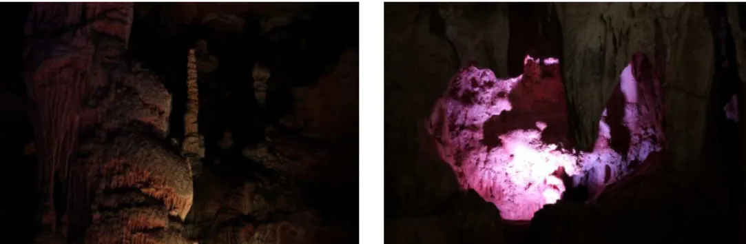
to approach more challenging environments such as Figure 1.3. One can extract geometric cues from 3D information to cope with illumination and texture absence. There is an

increas-ing demand for systems capable of mappincreas-ing and monitorincreas-ing complex environments such as

caves and mines which usually alternates between absence of illumination and wide

sky-opened natural structures. Those tasks nowadays relies on the usage of expensive and heavy

equipments, such as 3D laser scans and entire lighting structures to provide the necessary

4 CHAPTER 1. INTRODUCTION

Figure 1.3. Images from the inside of a cave, we can see that most of the image is lost due to illumination issues.

For this reason, RGB-D cameras can be of great help for such complex environments.

Although the relatively low range of approximately five meters, this low cost device can

easily be carried by mobile platforms, or even by humans. Nevertheless, we need a robust

keypoint detector algorithm to cope with these complex scenarios, such an algorithm needs to

be capable of function in both dark and illuminated environments, as well as take advantage

of geometry information to deal with textureless surfaces.

1.2

Objectives

We aim at building a novel RGB-D keypoint detection technique combining both intensity

and 3D information, capable of handling lack of illumination as well as dealing with

sub-stantial noise on both intensity and depth data, while maintaining a good computational

efficiency. The detector should also be robust to motion disturbances, such as rotation, scale,

and translational motion.

1.3

Contributions

The main contribution of this work is the creation and analysis of a keypoint detector called

KVD (Keypoints from Visual and Depth data) that efficiently combines intensity and depth

data. Besides addressing the properties set in Tuytelaars and Mikolajczyk [2008]:

• repeatability,

• distinctiveness/informativeness,

• locality,

1.4. ORGANIZATION 5

• accuracy and

• efficiency,

the proposed methodology also produces the best performing detector by using both visual

and geometrical data, and that still presents a good performance and graceful degradation

even in the absence of either one of them.

The results of this work were published at:

• Vasconcelos, L. O., Nascimento, E. R., and Campos, M. F. M. (2015). A scale invariant keypoint detector based on visual and geometrical cues. In Iberoamerican Congress on Pattern Recognition. IEEE.

1.4

Organization

We have organized this document into the following chapters:

• Chapter 2 - Related Work: This chapter we discuss important works in the literature

which is related with ours.

• Chapter 3 - Methodology: A thorough explanation of the method developed through

this work is given.

• Chapter 4 - Experiments: Explains the purposes and shows the results of several

dif-ferent experiments performed to access and understand the behaviour of our method.

• Chapter 5 - Conclusion: Closes this document with a conclusion, also discussing future

Chapter 2

Related Work

Several terms are used in the literature to describe a point of interest within an image which

presents high variation in its vicinity and it is stable for affine, rotational, scale and

illumina-tion transformaillumina-tion. Hereafter we will refer to such a point of interest as akeypoint. We also

use the term invariant from the literature to characterize keypoint detectors which present

stability for certain types of transformations, for example: we say a algorithm is scale

in-variant if the keypoints detector repeatability rate1 _{does not deprecate harshly under scale}

transformations.

In this section, we summarize several popular keypoint detector methods which relate to our work. They have been organized by their handled data type where extra attention has

been given to the methods we thought comparable to our developed technique. Although

we compare our method with several state-of-the-art approaches, we address two methods

as main concurrent: Harris 6D and ORB (Sections 2.1 and 2.3 respectively), which will be

presented and justified along this section.

2.1

Intensity 2D Images

The detection of keypoints in images is an essential component in a myriad of applications

in pattern recognition and computer vision algorithms. Since the seminal paper of Morevec

[1977], where he presented one of the first corner detectors, a large number of keypoint

detectors have been proposed. The basic idea of Moravec’s work was to select the points that have large intensity variations in specified directions. This variation is measured by

centering a rectangular window at the queried point and monitoring the average changes of

1_{repeatability rate is used to evaluate the performance of a keypoint detector under a specific}

transforma-tion, it will be thoroughly explained at Chapter 4

8 CHAPTER 2. RELATEDWORK

image intensityE while shifting the window towards a given(x, y)direction:

Ex,y = X

u,v

wu,v[I(x+u, y+v)−I(u, v)]2, (2.1)

wherewspecifies the window: it is one within a specified rectangular region, and zero

else-where. The functionI(u, v)stands for the(u, v)pixel intensity. Intuitively, if the point lies

in a flat region, then all shifts will result in low intensity variation. If it lies on an edge,

mov-ing across the edge will yield low intensity variation. However, if we shift perpendicularly

to the edge, a high intensity variation will be observed. Thus, to find corner pixels, one can

search for points with high intensity variation in every direction, or, in a more formal way,

when the minimum change produced by a shift is larger than a threshold.

2.1.1

The Harris Corner Detector

The above described methodology was later improved by Harris and Stephens [1988], where

they replaced the discrete shifted windows with the partial derivatives of the Sum of Squared

Differences (SSD). The authors noted that Equation 2.1 could be seen as:

E(x, y) = (x, y)M(x, y)T_{, (2.2)}

with the2_×2matrix:

M=

"

X2_⊗w (XY)_⊗w

(XY)_⊗w Y2_⊗w

#

, (2.3)

for:

X =I_⊗(₋1,0,1) = δI

δx,

Y =I_⊗(₋1,0,1)T ₌ δI

δy,

(2.4)

whereI denotes the intensity image and_⊗ is the convolution operator. Intuitively, this

ex-pands Moravec’s work to consider small shifts in every possible direction, a thorough

expla-nation of this fact is shown in Harris and Stephens [1988].

Analysing the matrixMas an auto-correlation matrix, its eigenvalues and eigenvectors

play an important role in estimating whether the target point is a corner. Intuitively, the eigenvectors point toward the directions of most significant intensity variations (maximum

and minimum). Thus, similarly to Moravec’s reasoning, a corner can be detected if the

smallest eigenvalue is above a given threshold.

2.1. INTENSITY 2D IMAGES 9

upon the eigenvalues of the correlation matrixM. To avoid the explicit eigenvalue

decom-position, which is an expensive operation, the response functionRis given as:

R =Det(M)₋k_×T r(M), (2.5)

whereDet(_·)andT r(_·)stands for the Determinant and Trace of the matrixMrespectively.

The Harris corner detector, as this approach is known in the literature, comprehends an

intuitively and powerful methodology for keypoints detection, since the method has several

desirable properties such as: rotational invariance, robustness to illumination changes, and

easily extendable for different data types, as we will present later. The main drawbacks of

Harris-like detectors is that they demand relatively high computational efforts to calculate

the correlation matrix, exhausting it for real time applications.

The Harris detector searches for keypoints in only one scale (defined by the window’s

size), which makes the method sensible to scale transformations. In order to tackle this

issue, a modified version of the Harris detector, known as Harris-Laplacian, was proposed

by Mikolajczyk and Schmid [2004], the authors exploited the response function of the Harris

detector to make it invariant to scale changes. To achieve this, the Harris cornerness response

is accessed in a set of different scales for each queried point. The automatic scale selection is

performed by following the methodology proposed by Lindeberg [1998], where the correct

scale is chosen according to the local maximum of the cornerness response within the scale

space. Even though this new version presents some invariance to changes in scale, it returns low distinctive keypoints and considerably increases the computational time.

2.1.2

The SIFT Detector

One of the most popular modern algorithm that detect distinctive, small illumination changes as well as camera viewpoint changes is the SIFT algorithm Lowe. [2004]. This technique

extracts features using local gradients and estimates a characteristic orientation and the scale

of the keypoint’s neighborhood to provide rotational and scale invariance.

The algorithm firstly builds a scale pyramid by repeatedly applying Gaussian filters

and sub-sampling the original image. Once the pyramid is built, the authors approximate the

scale-normalized Laplacian of Gaussian filter by performing Difference of Gaussians (DoG)

among subsequent pyramid levels. To select one point as a keypoint candidate, the point needs to be an extrema (maximum or minimum) among its neighbouring pixels, both in the

image and scale space.

Later, the keypoint candidates are tested for high contrast and cornerness. For the

10 CHAPTER 2. RELATEDWORK

candidate, and depending on the quality of the fit, the point is rejected. For the cornerness

test, the keypoint is tested similarly to the Harris cornerness function response. The main

drawback of this algorithm is the high need of computational resources.

2.1.3

Machine Learning Techniques

A recent approach that has become popular is based on machine learning techniques. Dias

et al. [1995] deployed a Neural Network based Sub-Image Classifier (NNSIC) to detect

corners. Their algorithm receives an 8_× 8 window from the input image and outputs a

binary image indicating the presence or absence of a corner. One of the key contributions of

using an artificial neural network was to show the capability of this approach in providing a

way to compute a generalized representation for a corner.

Following the machine learning approach, Rosten and Drummond [2005] proposed the Features from Accelerated Segment Test (FAST) detector, an interest point extractor

from intensity images, which considers a circle around the queried point and analyses the

intensity differences between the pixels at the arc and the central point to decide whether the

queried point is a keypoint or not. In Rosten and Drummond [2006], the authors extended its

previous work by training a decision tree, which takes the intensity differences as features, to

learn the FAST detector, improving severely the efficiency of the method. Finally, in Rosten

et al. [2010] was applied simulated annealing to optimize the decision tree. The search

is performed by randomly modifying an initially trained decision tree and monitoring how

well the modified tree behaves concerning repeatability and efficiency.

Although FAST algorithm was designed to be a low-cost algorithm, it shows reliable

results concerning repeatability under illumination change, noise corruption and translational

motion. As drawbacks, the method shows sensitivity regarding scale transformation and

rotational motion. The method also lacks a reliable keypoint response function, relying on a

simple average of the pixels lying at the ring.

In order to cope with the above mentioned issues, the work of Rublee et al. [2011]

presented a novel detector called Oriented FAST and Rotated BRIEF (ORB) that builds

upon FAST’s methodology. To deal with the scale sensitivity problem, the authors deployed

the method suggested by Lindeberg [1998], adopting the Harris cornerness response instead of FAST’s response. A scale pyramid is employed and the correct scale is chosen as the one

maximizing the Harris response within the pyramid space.

The scale pyramid is carried out by subsequently smoothing and sub-sampling the

image. For each pyramid level, the authors ran the FAST keypoint detector and evaluate

them using the Harris response. For each detected keypoint, the chosen scale will then be

2.1. INTENSITY 2D IMAGES 11

To account for rotational invariance, the authors were inspired by Rosin [1999]. They

defined the corner orientation based on intensity centroids. The moments of a given patch

are defined as:

mpq = X

x,y

xpyqI(x, y). (2.6)

The centroid is then calculated as:

c=

m10

m00

,m01 m00

. (2.7)

The corner orientation is then given by the vectoroc~ . Whereostands for the corner’s center.

The corner orientation is now calculated as:

θ=atan2(m01, m10), (2.8)

where atan2 is the quadrant-aware version of arctan.

The ORB detector is a state-of-the-art algorithm, albeit designed only to 2D intensity images, it is quite robust being invariant to rotation, illumination changes and scale

transfor-mation, while maintaining a low computational cost. Due to this robustness we chose this

algorithm for a more detailed comparison with our method.

A similar approach to ours is carried by Hasegawa et al. [2014], where the authors

enhanced the FAST methodology implementing a cascade of decision trees to classify a

target point as a corner. The idea is to avoid badly classified corners through analysing a

bigger vicinity and checking the corner consistency among the consecutive pixels.

The region analysed consists of three concentric Bresenham’s circles of growing radii

(r1 = 3, r2 = 4andr3 = 5). For each radius, a decision tree is trained, just like the FAST

methodology. A point is classified as a keypoint if considered as a true keypoint by all three

decision trees and if the corner orientation matches in all analysed circles.

The corner orientation for each analysed Bresenham’s circle is calculated based on the

sequence of all brighter or all darker consecutive pixels as shown in Figure 2.1.3. A positive

keypoint is considered if, besides being classified by all decision trees as positive, all those

orientation directions point approximately toward the same direction. The algorithm is then

12 CHAPTER 2. RELATEDWORK

2.2

Point Clouds and Range Images

Extracting data from images can usually provide rich information on the object features,

but geometrical information produced by 3D sensors based on structured lighting or time of

flight is less sensitive to visible light conditions. Three-dimensional data has been

success-fully exploited by algorithms such as NARF Steder et al. [2011], which has been proposed

to extract features from 3D point cloud data for object recognition and pose estimation.

NARF’s approach is based on a set of points classified as stable, and the explicit use of

border information.

The benefits of using three-dimensional data have led to the proposal of several 3D

detectors implementations derived from 2D approaches, some examples of these are SIFT3D

and HARRIS3D Rusu and Cousins [2011]. In general, these three-dimensional variations

consist in replacing gradient images by surface normals. These methodologies are useful

mainly for unordered 3D point clouds.

A machine learning based method for keypoint extraction from depth maps is detailed at Holzer et al. [2012]. The authors make use of a random forest to approximate a specially

tailored response function which takes advantage of the curvature and the repeatability of

each point. Each tree of the forest implements several queries concerning the depth

compar-ison between different points in a given vicinity centred at the queried point. The response

function is constructed by combining the curvature response and the repeatability of each

point, such repeatability is computed by the reconstruction of the training set images

se-quence.

2.3. MULTIPLE CUES 13

2.3

Multiple Cues

2.3.1

Descriptors

The use of multiple cues, such as visual and geometric features, is growing popular among

descriptor techniques. Kanezaki et al. Kanezaki et al. [2011] combined depth and visual

into a global descriptor, called VOSCH, in order to increase the recognition rate. Local

descriptors such as BRAND and BASE Nascimento et al. [2013], Color SHOT Tombari et al. [2011] and MeshHOG Zaharescu et al. [2009] also combines the visual information to

improve matching quality.

2.3.2

Keypoint Detectors

A keypoint detector that goes in the same fashion, making use of both visual and

geomet-ric informations, is the Harris 6D. As far as we know, it is an unpublished work that is

implemented by Rusu and Cousins [2011]. The Harris 6D methodology follows the same

reasoning of the original Harris corner detector, the extension relies on the construction of

the correlation matrix, which takes into consideration both RGB (red, green and blue) and 3D

Euclidian spaces. Each instance on the RGB space stands for an image pixel color, while the

3D Euclidian space is crowded by the normal vectors of each 3D point composing the point

cloud. This detector inherits all properties from the Harris corner detector and adds illumi-nation independence, since it operates also on the point cloud, which is independent from

the intensity image. It is a very stable detector in spite of its sensitivity to scale changes. The

Harris 6D merges both visual and geometry information and is a commonly used keypoint

detector. For those reasons we select this method as the main competitor to our proposed

approach.

2.4

Summary

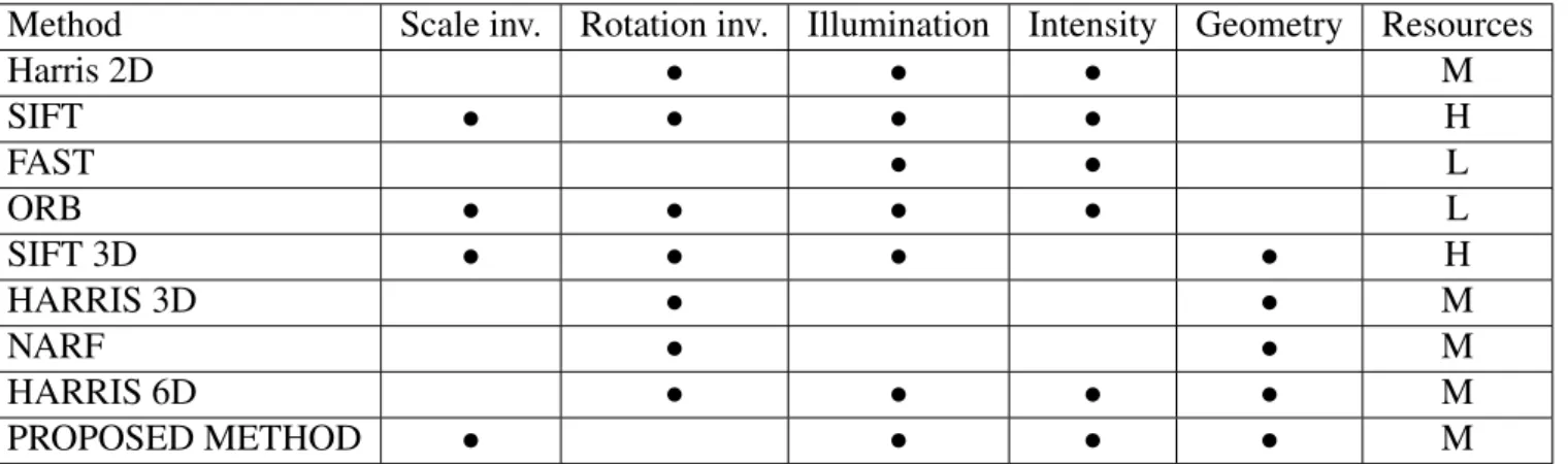
The previously presented information is summarized at Table 2.4

In this work, we follow a similar approach to Harris 6D for the keypoint detection

problem. Our technique leads to the synthesizing of a detector which simultaneously

con-sider both visual and geometrical information to classify points as a keypoint. This

detec-tor excels both in its low computational cost and its high repeatability rate with no loss in

performance of the other desirable features set out by properties defined in Tuytelaars and

14 CHAPTER 2. RELATEDWORK

Method Scale inv. Rotation inv. Illumination Intensity Geometry Resources

Harris 2D _{• • •} M

SIFT _{• • • •} H

FAST _{• •} L

ORB _{• • • •} L

SIFT 3D _{• • • •} H

HARRIS 3D _{• •} M

NARF _{• •} M

HARRIS 6D _{• • • •} M

PROPOSED METHOD _{• • • •} M

Chapter 3

Methodology

In this chapter we detail the methodology of the proposed KVD keypoint detector, which is

based on a machine learning approach for keypoint detection, similar to other works in the

literature (Rosten et al. [2010]; Rublee et al. [2011]). However, differently from their work,

we assume that both 3D and visual data are available to the detection process, which enables

our detector to work even in the absence of image data.

The input of our algorithm is a data pair(I,D), which denotes the output of a typical

RGB-D device, where I andD are the intensity and the depth matrices, respectively. Let

x= (i, j)denotes a pixel’s coordinates,I(x)the pixel’s intensity,D(x)is the depth for that

pixel,P(x)is the corresponding 3D point, andN(x)is its normal vector.

As stated, our technique is built upon a supervised learning approach, with a training step where a decision tree is created. This decision tree plays a key role in the detection

procedure, since it is used to classify points into keypoints. There are four steps in this

clas-sification process: the surface’s normal estimation, the feature vector extraction, the model

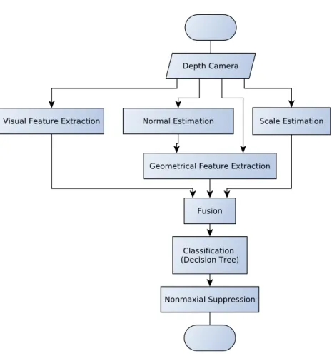
training, and the non-maximal suppression. An overview of the process can be seen in

Fig-ure 3.1.

3.1

Surface’s Normal Estimation

To calculate an approximation of the surface’s normal for each point, we need to analyse

the relationship of the target point with nearby points from its vicinity. Once the surface’s

normal vector is estimated we can evaluate geometrical information of the surface in local

patches. This information is leveraged to improve the quality of the selected keypoints.

There are several methods to estimate the normal vectors from a point cloud [Klasing

et al., 2009]. One accurate approach consists in performing Principal Component Analysis

(PCA) on the3_×3covariance matrixCof a small vicinity_Karound the target point.

16 CHAPTER 3. METHODOLOGY

Figure 3.1. The algorithm’s flow chart. After estimating a scale and extracting both visual and geometric features, the algorithm assembles this information in a final feature vector which is further classified by a decision tree into keypoints candidates or not. Finally the algorithm performs nonmaximal suppression to avoid multiple detections in a small patch.

The vicinity_K plays an important role on this process. The analysed vicinity should

be large enough to cope with noisy points, and small enough to represent the plane within

the required details. Thus, the sensor’s resolution must be taken into account. As a golden

rule, we should pick the vicinity just large enough to handle the necessary quality of details

for the application. The covariance matrixCis computed as:

C = 1 |K|

X

pi∈K

(pi−p)(p¯ i−p)¯ T, (3.1)

where p¯ is computed as p¯ = 1

|K|

P

pi∈K

pi. We take the eigenvector that is assigned to the

smallest eigenvalue of C as the surface’s normals estimation. This vector represents the

direction towards the data that has the lowest variance. For example, in a planar surface with

3.2. FEATURE VECTOR EXTRACTION 17

be seen as a plane fitting among the neighbouring points.

The computation of the neighbouring points is of extreme importance for the method’s

accuracy. Since poorly selected points may not properly represent the targeted plane. An

accurate solution is to select the vicinity as the points lying within a sphere of radiusk,

cen-tered at the queried point. Although this provides good estimates for the normal vectors, the search for neighbouring points in non-indexed point clouds is an computationally expensive

operation, even when using of spacial data structures such as octrees, kd-trees, etc.

In order to speed the vicinity search, it is possible to exploit the matrix structure of a

depth image and represent the vicinity as the pixels lying within a rectangular region centered

at the queried point. This method, although much faster, results in estimated normal vectors of lower quality.

Both methods are implemented in Rusu and Cousins [2011]. We performed

experi-ments using both normal estimation methods, which can be found in Chapter 4.

3.2

Feature Vector Extraction

The first step of the detection process is to create a feature vector for every point, which will

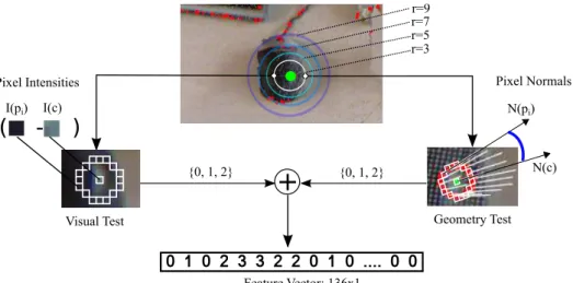
be fed into a decision tree for classification. Figure 3.2 shows a representation of the feature

vector construction.

To decide if a given pixel is a keypoint, we analyze a circular vicinity of the given point

in increasing radii, as depicted in Figure 3.2. The figure refers to the radii set_S =_{3,5,7,9_},

which is the settings used in our experiments. It is worth noting that the algorithm is defined

for any arbitrary set_S.

Given an image pixel’s coordinates c _{∈ R}2, we consider its vicinity as the image

patches containing the circles centred atcwith radii varying inr_{∈ S}. Each circle is defined

by the functionB(r,c)which we denote asBr(c):

Br(c) :R3 → {p1,p2, ...,pn}. (3.2)

TheBr(c)map function outputs all pixelspi lying within the Bresenham’s circle

[Pit-teway, 1967] with radius equal tor. Thus, the total vicinity considered consists of the

con-catenation of all vectorsBr(c),∀r∈ S. We define the vicinity of a central pixelcas

Vc ={Br1(c), Br2(c), . . . , Br|S|(c)}, ∀ri ∈ S. (3.3)

For instance, in our implementation we use four fixed radii of sizes_S = _{3,5,7,9_}.

18 CHAPTER 3. METHODOLOGY

+

0 1 0 2 3 3 2 2 0 1 0 .... 0 0

Feature Vector: 136x1

Geometry Test Visual Test

( - )

{0, 1, 2} {0, 1, 2}

Pixel Intensities Pixel Normals

N(pi)

N(c) I(pi) I(c)

r=3 r=5 r=7 r=9

Figure 3.2. Visual and geometrical feature extraction for a keypoint. The highlighted squares correspond the Bresenham’s circle.

analysed, consisting of the circles computed byB3,B5,B7,B9, each with 16, 28, 40and52

pixels. Figure 3.2 shows the four Bresenham’s circles. The circle with radius3is denoted

by red squares. For each vicinity elementp_{∈ V}c, we compute visual and geometric features.

3.2.1

Feature Computation

The visual features are computed based on simple intensity difference tests among a carefully

chosen vicinity, reducing the memory consumption and processing time. For each pixel

p_{∈ V}cwe evaluate

τv(c,p) =         

2, ifI(p)₋I(c)<₋tv

1, ifI(p)₋I(c)_≥tv

0, otherwise,

(3.4)

wheretv represents a toleration threshold (tv = 20in our settings). This function analyses

the intensity relationship between both pixelscandp, encoding whether the pixel intensity

I(p)is darker, lighter or at similar intensity regarding the pixel intensityI(c), respectively.

The visual feature extraction implemented by the function τv is similar to the one

described in Rosten et al. [2010], however we embed geometric cues into our feature vector

to increase robustness to illumination changes and to the lack of texture in the scenes.

Geometric feature extraction is performed by the τg(.) function. This process is

de-picted in Figure 3.2. It is based on two invariant geometric measurements:

3.2. FEATURE VECTOR EXTRACTION 19

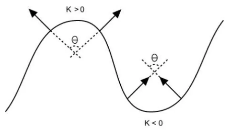
Figure 3.3. The dot product between surface normals is ambiguous, but they have

op-posite curvature signs, which is captured by the functionκ(·).

• the surface’s convexity.

While the normal displacement test is performed to check whether the dot product between

the normalsN(c)andN(xi)is smaller than a given displacement thresholdtg, the convexity

test is accomplished by the local curvature indicator,κ, estimated as:

κ(c,pi) = hP(c)−P(pi), N(c)−N(pi)i, (3.5)

where _h._i is the dot product, and P(c) is the3D spatial point associated with pixel p and

depthD(p). Theκfunction is used to capture the convexity of geometric features and also

to unambiguously characterize the dot product between surface normals. The sign of the

functionκdenotes whether the surface between the two points accessed is convex (positive

signed) or concave (negative signed), as shown in Figure 3.3.

Thus, the geometrical features are computed by analysing the behaviour of the surface

between two points:

τg(c,pi) = 

   

   

2, if_hN(pi), N(c)i< tg∧κ(c,pi)>0

1, if_hN(pi), N(c)i< tg∧κ(c,pi)<0

0, otherwise.

(3.6)

Intuitively, it encodes whether the surface between the central pixelcand the queried

pointpi is convex, concave or plane, respectively. We consider a plane ifhN(pi), N(c)i ≥

20 CHAPTER 3. METHODOLOGY

3.2.2

Scale Invariance

Scale invariance is endowed to our detector by taking advantage of the geometry

informa-tion available, in order to weight the Bresenham’s circles of different radii. We analyze the

geometrical vicinity encompassed by each Bresenham’s circle Br(c) in the 3D scene, by

computing the minimum Euclidean distance among all vectors v = P(c)₋ P(pi), with

pi ∈Br(c):

dr =min pi k

P(c)₋P(pi)k, (3.7)

whereP(c)andP(pi)are the 3D points corresponding to the central pixel cand the pixels

composing the Bresenham’s circlepi ∈Br(c).

The minimal distancedris taken as an estimative of the circle’s radius in the 3D scene.

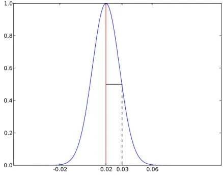
It is then weighted by the unidimensional-Gaussian function, in order to penalize circles

which its estimated radii in the 3D scene are distant from µ = 0.02 meters, a predefined

radius which seems as a reasonable value for our application.

wr = exp

−(u−dr)

2

2σ2

, (3.8)

the standard deviationσ = 0.011 was empirically chosen, targeting a sufficiently narrow

shape around the mean value. This curve can be seen in Figure 3.4.

-0.02 0.02 0.03 0.06

0.0 0.2 0.4 0.6 0.8 1.0

Figure 3.4. Gaussian curve penalizing 3D scene radii lying further from the meanµ=

3.2. FEATURE VECTOR EXTRACTION 21

The weighting procedure avoids the addition of noise by circles covering

non-interesting areas, e.g. points too far from the camera, larger circles might have to be strongly

penalized.

3.2.3

Final Feature Vector

In order to combine the geometric and visual information in one final feature vector, we

deployed two different approaches:

3.2.3.1 The Additive Approach

This method combines both cues by adding both visual and geometric feature vectors. We

extract a feature vector from a Bresenham’s circle of radiusr centered atcas a row vector

~

vr = h

f1 f2 . . . f|Br(c)| i

where eachfi ∈~vr is given by:

fi(c, r) = wr∗(τv(c,pi,r) +τg(c,pi,r)), (3.9)

wherepi,ris theith element of the respective Bresenham’s circleBr(c).

The final feature vectorF~ is generate by concatenating all the feature vectorsvras:

~

F=h ~vr1 ~vr2 · · · ~vr|S|

i

∀r_{∈ S}. (3.10)

3.2.3.2 The Concatenation Approach

To combine both informations in this approach, we concatenate two vectors, where one

encodes visual features and the other geometrical features. We will depict the visual vector

~

Fv construction, while the geometric vector~Fg follows a similar process.

For each Bresenham’s circle, a row feature vector ~vr =

h

f1 f2 . . . f|Br(c)| i

, is

computed where eachfi ∈~vris calculated as:

fi(c, r) = wr∗τv(c,pi,r), (3.11)

then, the visual feature vector_F~v is defined as:

~

Fv = h

~

vr1 ~vr2 · · · ~vr|S|

i

∀r_{∈ S}. (3.12)

The geometric feature vector F~g follows the same logic, but applying the function

τg(·) instead of τv(·) in Equation 3.11. Finally, the final feature vector ~F consists of the

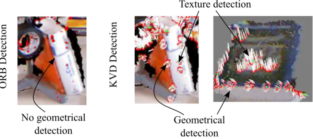
22 CHAPTER 3. METHODOLOGY Texture detection Geometrical detection OR B D et ec tion No geometrical detection KV D D et ec tion

Figure 3.5.Comparison between keypoints detected by our methodology (right images) and ORB algorithm (left image). One can note the absence of keypoints around the border of the book in the right image. Since KVD captures both visual and geometrical features to find keypoints it is capable to detect such keypoints.

~

F=hF~v, ~Fg i

. (3.13)

3.2.4

Fusion Processes Discussion

The concatenation approach yields a final feature vector of length equals to 2_|V|. From

the one hand, this approach maintain all information extracted during the feature extraction process, on the other hand, the final feature vector is twice as long as the final vector of the

additive approach, which impacts on the computational time performance. We performed

experiments to compare both approaches which is shown in Chapter 4.

Due to the fusion process, our method is able to detect keypoints using both visual and

geometrical data. Figure 3.5 depicts detected keypoints exploiting the fused information.

3.3

Decision Tree Training

The decision tree is a fundamental part of the algorithm, it is used to decide whether a target

point should be considered as a keypoint candidate or not. In order to do that, we select a

sample of training points. This sample contains both keypoints and non-keypoints examples properly labeled. Further, we use this set as a keypoint-model to train a decision tree for

predicting whether an addressed point is a keypoint.

The decision tree algorithm was chosen because, differently from other classical

ma-chine learning algorithms, the decision tree can be straightforwardly converted into a

3.4. NON-MAXIMAL SUPPRESSION 23

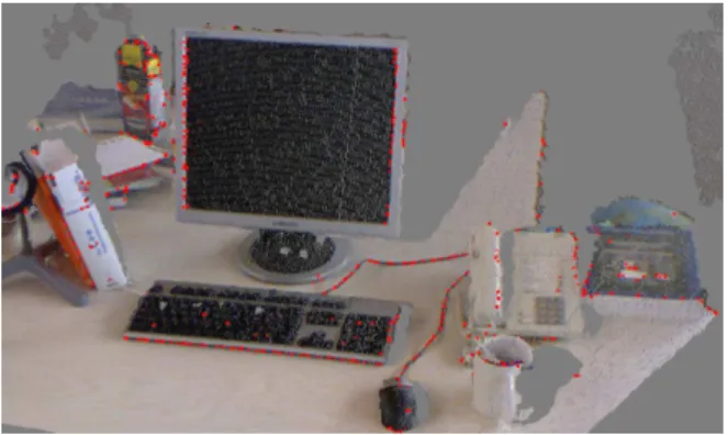
Figure 3.6. Example of images from the RGB-D Berkeley 3-D Object Dataset (B3DO), where the right images shows the smoothed depth map. Figure taken from http://kinectdata.com/

Table 3.1.Confusion matrix of keypoint classification based on a decision tree.

Keypoint Non-Keypoint

Keypoint 0.89 0.11

Non-Keypoint 0.08 0.92

In the training step, we created a training set by extracting a total of160,144 points

from the RGB-D Berkeley 3-D Object Dataset (B3DO) Janoch et al. [2011]. This dataset is

publicly available1 _{and it is composed of a large number of real world scenes with several}

different objects, geometry and visual data. The images were captured with a KinectTMsensor

at a resolution of640_×480pixels and all the depth maps had been smoothed. An example

of the dataset is shown in Figure 3.6.

3.4

Non-Maximal Suppression

The last step in our methodology is to perform a non-maximal suppression. This step avoids the algorithm from finding redundant keypoints. To achieve this we rank the keypoint

candi-dates (classified as positive by the decision tree) lying within a small image patch. Selecting

as the true keypoint the candidate with highest score among the patch.

Although the visual and the geometrical tests do not provide a response value, it is still

possible to perform a non-maximal suppression based on the values of the features. In order

to do so we need to define the set

Xrck ={pi : pi ∈Br(c) ∧ (τv(c,pi) =k ∨ τg(c,pi) = k)}, (3.14)

which contains all the pixels within a Bresenham’s circle Br(c)whose geometry or visual

24 CHAPTER 3. METHODOLOGY

feature has valuek.

For each radiusr_{∈ S}, we calculate the partial responseRp(c, r)as:

Rp(c, r) = max

X ∈{Xrc₁,Xrc₂}

1 |X |

X

xi∈X

Dv(c,xi) +λDg(c,xi)

, (3.15)

where

Dv(c,x) = |I(x)−I(c)|

Dg(c,x) = 1− hN(x), N(c)i

(3.16)

give the visual and geometrical responses respectively. The factor λ is used to define the

contribution of the geometrical information into the response.

The final response is then defined as the maximum response among all radii:

Rf(c) =max

r Rp(c, r)

,_∀r_{∈ S}. (3.17)

Equation 3.17 uses both the absolute difference between intensities and the normal

surface angles for the pixels in the contiguous arc of the Bresenham’s circle as well as the keypoint candidate to rank the maximal points.

Next, we divide the image into smaller patches with sizew_×w(in this work we use

Chapter 4

Experiments

This chapter details how we evaluate and compare our approach to other literature from

the field. We performed several experiments to evaluate the behaviour of our detector. In

order to analyse its repeatability, distinctiveness, robustness and time performance we

com-pared our approach against standard ones for two-dimensional images, SIFT Lowe. [2004],

ORB Rublee et al. [2011], and SIFT3D (using all three color channels), for geometric data Harris3D (a 3D version of Harris corner detector) and NARF Steder et al. [2011], and the

Harris6D, which similarly to our methodology, uses both visual and geometrical data to

de-tect keypoints. The implementation of the later three methods can be found in Rusu and

Cousins [2011].

4.1

Dataset

We performed experiments with two different datasets. We used the RGB-D SLAM Dataset

and the Benchmark presented in Sturm et al. [2011] to evaluate the behaviour of the

meth-ods regarding image changes in translation, scale, and rotation in both the image (roll) and

horizontal (yaw) planes. This dataset is publicly available1 and contains several real world

sequences of RGB-D data captured with a KinectTMsensor. Images were acquired at a frame

rate of 30Hz and a resolution of 640_×480 pixels. Each sequence in the dataset provides

the ground truth for the camera pose estimated by a motion capture system, which allows the computation of the homographies relating each image pair by a plane projective

transforma-tion.

We separated a different sequence of images for each camera motion type, as can be

seen in Figure 4.1. The translational changes Figure 4.1 (a) were produced by shifting the

1_{https://cvpr.in.tum.de/data/datasets/rgbd-dataset}

26 CHAPTER4. EXPERIMENTS

(a)

(b)

(c)

(d)

Figure 4.1. Samples of the image sequences of the different transformation changes, where (a) is the translational , (b) is the scale, (c) is the rotation in the image plane, and (d) is the rotation in the horizontal plane.

sensor along the horizontal axis with an maximum offset of0,75meters. The scale changes

(b) were acquired by moving the camera away from the scene where the maximum shift is

approximately0,40meters. The image rotations (c) and (d) vary from 0,5 to180 degrees

for the roll axis, and0,5to35degrees around the yaw axis.

In order to test the algorithms for illumination changes, we built a dataset by capturing

4.2. DECISION TREE TRAINING 27

Figure 4.2.Samples of the illumination sequence.

of one minute between acquisitions. The images were captured using a KinectTM_{sensor with}

the resolution setted to640_×480pixels standing at a fixed position, as shown in Figure 4.2.

We will furthermore refer to this dataset asVerlab_Dusk.

4.2

Decision Tree Training

For the Decision tree training, we assigned 66% of the points from the training set and

the remaining points (54,449) to test the quality of the final decision tree. Both sets were

equally divided into positive and negative samples. In order to define the threshold of the curvature for a positive keypoint, we computed the curvature of several, manually selected,

positive keypoints. We have found the value of0.09based on the average of these curvatures.

Thus, all the points with curvature larger than 0.09were labeled as positive samples for the

keypoint class. To take visual features into account, we also add keypoints detected by ORB

as positive examples. The final confusion matrix is shown in Table 3.1.

4.3

Evaluation and Criteria

We evaluate and compare our method to others from literature regarding three concepts:

Robustness, Distinctiveness and Time performance. In order to assess the Robustness of the

methods, we use the Repeatability criterion. In the graphics, both KVD and Concatenation

represents our methods which respectively implements the additive and concatenation fusion

approaches.

4.3.1

Repeatability

One of the most important properties of a keypoint detector is its ability to find the same set

of keypoints on images acquired of a scene from different view points. Thus, to evaluate

and compare the robustness of KVD detector with other approaches, we applied the same

28 CHAPTER4. EXPERIMENTS

The repeatability score for a pair of images is computed as the ratio between

corre-sponding regions of the keypoints in two frames and the smaller number of keypoints in

these frames. To calculate the number of corresponding regions between framesiandi+ ∆,

let_Kibe the set of keypoints found in imagei. To compute the correspondence we define

KG

i→(i+∆) ={Hi→(i+∆)ki;∀ki ∈ Ki} (4.1)

as the ground-truth set which represents the projection of the keypointski ∈ Ki (keypoints

found in frame i) onto the framei+ ∆, where H is the homography matrix relating both

frames.

Thus, for each keypoint kG_{i ∈ K}G_i→(i+∆) we define an elliptic region RkG

i centered

atkG_i with radius proportional to its normalized scale (we refer the reader to Mikolajczyk

et al. [2005]). A correspondence is found if the overlap error between R_kG

i and Rki+∆ is

sufficiently small:

1₋ Rk

G

i ∩Rki+∆

R_kG

i ∪Rki+∆

< ǫ,

whereRki+∆ is the elliptic region centered at location of keypointkin the framei+ ∆. In

our experiments,ǫ= 0,4.

An important factor to be considered is the coverage area, which is the area covered

by all keypoints found. For a fair comparison, we adequately adjusted the threshold of all

detectors since they return the closest approximation to500keypoints per frame.

4.3.2

Robustness

To test for robustness we evaluate the repeatability of the methods over several

transforma-tions: translational, scaling, rotational and illumination as well as artificial corruptions to

contrast, brightness and added noise in both the visual image and the normal estimation.

In order to corrupt the contrast and brightness of an image we apply multiplication and

addition with constants of increasing values:

¯

I(x, y) =αI(x, y) +β,

whereI¯is the corrupted image, α is the gain, which adjusts image contrast, and β is the

bias that controls brightness. For the added noise we used a Gaussian distribution with zero

mean. Examples of these corruptions are represented in Figure 4.3.

For each transformation test, we compute the repeatability score under a specific image

4.3. EVALUATION ANDCRITERIA 29

(a) Contrast

(b) Brightness

(c) Noise

Figure 4.3.Examples of the impact of the corruptions applied to an image

affected by the targeted transformation. The repeatability score is calculated among all

se-quence pairs of the form(q0, qi), whereq0, qi ∈Qt.

In order to avoid occlusion effects in motion related transformations, for every

se-quence pair(q0, qi)we consider only the portion of the image that is common for both frames

q0 andqi. To achieve this, we build a binary mask by projecting the first frameq0 onto the

camera position relative to frame qi. Then, for a pixel (i, j) of the mask: it is one if any

projected point lies on it, and zero otherwise. We apply the keypoint detectors only on pixels

where its corresponding (same coordinates) mask pixel has value equal to one.

The mask step is performed to prevent the repeatability rate from dropping due to un-related issues (like object occlusion), instead of from the analysed transformation. A similar

precaution was taken regarding the image corrupted tests (contrast, brightness and noise). To

make sure the experiment is evaluating the algorithm’s robustness to image corruption, we

compute for each sequence positionqnthe average of the repeatability score of10

consecu-tive pairs(qn, qi), wherei∈[n+ 1, n+ 10], thus we can assure that the repeatability rate is

30 CHAPTER4. EXPERIMENTS

To account for normal estimation noise we use two different methods, as discussed in

Chapter 3. In order to assess how sensible each method is regarding the normals quality,

we selected from thefreighburg_xyz2dataset 50 sequences of 10 consecutive images_Qx =

{qx1, qx2,· · · , qx10}at random, totalling 500 elements. We run KVD, Harris3D and Harris6D

with both coarse and accurate normal estimations, and calculate the repeatability scores over

all pairs(qn0, qni), whereqn0, qni ∈ Qn for each of the 50 sequences. Further we calculate

the differences between both coarse and accurate repeatability results for each method. A

robust method should offer a lower variance when compared to itself using a different normal

estimation method. Thus we evaluate the normal noise robustness by assessing the variance of this difference.

4.3.3

Distinctiveness

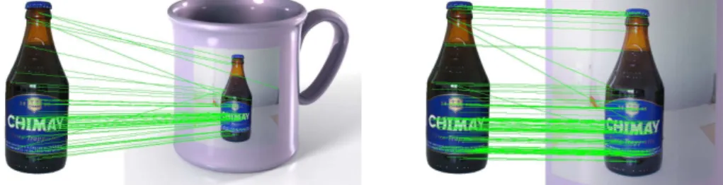
The keypoints distinctiveness evaluates the detector capability to find good features for a

matching task for 2D descriptors (ORB and BRIEF Tombari et al. [2010]), 3D descriptors

(FPFH Rusu et al. [2009] and SHOT Tombari et al. [2010]) and 2D + 3D descriptors BASE

and CSHOT.

In order to evaluate the discriminative power of KVD detector, and to compare it against other approaches, we matched pairs of keypoints from several pairs of different

im-ages by using a brute force algorithm and feature vectors extracted by all these descriptors.

4.3.4

Time Performance

For time performance, we assess the processing time of the compared methods by averaging

the detection time of900 runs over entire images. The detection time was measured while

the experiments were running on an Intel Core i7 3.5GHz (using only one core) processor

running Ubuntu 12.04 (64bits).

4.4

Parameter Settings

In this section, we analyse the best parameter values to be used by our detector.

We chose the radii set_S = _{3,5,7,9_}as it represents well the scale spectrum, given

that the Kinect’s reach for the depth image ranges from 0.3 to 5 meters. It seems as a good

balance between time performance and robustness.

In order to choose a value for the geometric threshold tg, we ran the learning and

testing phases for15, 30and60degrees. As shown in Table 4.1, the value which returned

4.5. RESULTS 31

Table 4.1.Accuracy for different geometrical thresholds.

Detector tg = 15o tg = 30o tg = 60o

Additive (KVD) 0.90 0.82 0.87

Concatenation 0.91 0.86 0.90

Geometric only 0.83 0.78 0.85

Visual only 0.75 0.78 0.76

additive and concatenation combination. We chose to use the additive combination, since

the concatenation spends twice the memory as the additive and the difference in their test

accuracy was of one percentage point, and also shows better robustness to image corruptions

noise (noise, brightness and contrast) as we will show in Section 4.5.

We experimented with different methods for combining the geometric and visual fea-tures. Figure 4.4 shows the scale robustness evaluation for four different methods: additive

(KVD), concatenation, texture only, and geometric only. We can see that fusing

informa-tion yields a stronger keypoint detector. We further examine KVD versus concatenainforma-tion by

testing for different transformation.

0.00 0.07 0.14_meters0.21 0.28 0.35 0.0

0.1 0.2 0.3 0.4 0.5 0.6 0.7 0.8 0.9

Repeatibility (%)

KVD

CONCATENATION GEOMETRIC ONLY TEXTURE ONLY

Figure 4.4.Scale test evaluating our method for four different feature vector extractions. The image shows that combining both visual and geometric information yields a stronger keypoint detector.

4.5

Results

32 CHAPTER4. EXPERIMENTS

0 20 40 60 80 100 120 140 160 alpha 0.0 0.1 0.2 0.3 0.4 0.5 0.6 0.7 Repeatibility (%) KVD CONCATENATION HARRIS6D SIFT SIFT3D HARRIS3D ORB NARF

0 20 40 60 80 100 120 140 beta 0.0 0.1 0.2 0.3 0.4 0.5 0.6 0.7 0.8 Repeatibility (%) KVD CONCATENATION HARRIS6D SIFT SIFT3D HARRIS3D ORB NARF

(a) Contrast (b) Brightness

0 20 40 60 80 100 120

σ 0.1 0.2 0.3 0.4 0.5 0.6 0.7 0.8 Repeatibility (%) KVD CONCATENATION HARRIS6D SIFT SIFT3D HARRIS3D ORB NARF (c) Noise

Figure 4.5. Detector robustness experiments for (a) Contrast; (b) brightness changes and (c) Gaussian Noise.

4.5.1

Robustness

We evaluated each detector for robustness to translational, scaling, rotational and

illumina-tion as well as artificial corrupillumina-tions to contrast, brightness and added noise.

We selected four sequences from the datasets to be used in our experiments, as previ-ously explained in Section 4.1:

• freiburg2_xyz: Kinect sequentially moved along the x/y/z axes. We used a sequence

with difference from3mm to0.75meters (horizontal direction) for translational tests.

For scale tests we selected another set of frames with the camera moving away from

the scene up to0.35meters;

4.6. DISCRIMINATIVE POWER ANDTIME PERFORMANCE 33

Detector µ σ

KVD 0.00515 0.00055

HARRIS6D 0.00523 0.00063

HARRIS3D 0.2 0.00395

Table 4.2. Table summarizing the meanµand variationσof the difference when using

an accurate and a coarse normal estimation, we can see that KVD and HARRIS6D had the best performance.

to35and180degrees around the yaw and roll axes, respectively.

• Verlab_Dusk: Standing still Kinect capturing images at a rate of one per minute,

start-ing at dusk (partial illumination) totallstart-ing104captures.

Figure 4.6 shows the results of the motion tests: translational (a), scale (b) and both

rotations (c) and (d), as well as the illumination change experiment. Our detector performs

better than other approaches in most of the presented sequences. It provides the highest

repeatability rate when there are large translational movements (0.7meters) and large yaw

angular rotations (35degrees). A summary of the performance for all detectors is shown in

Table 4.3. We can see that for most of the experiments the KVD detector presents the higher

repeatability rate.

The results for the illumination change experiment can be seen in Figure 4.6 (e). The

figure shows that only KVD and HARRIS3D (which uses only 3D data), were capable to

continue to provide keypoints under low illumination. Although HARRIS6D combines both

geometric and visual cues like KVD, it reveals much more dependence on visual features

than our proposed method.

In Figure 4.5 shows that our detector presented the largest repeatability rate in the

majority of the tests, followed by HARRIS3D. Since our detection methodology considers

visual and geometric information, we were able to detect keypoints even in the absence of

visual data (α >10) or when the image was completely saturated (β >45). Once again we

can notice the HARRIS6D visual dependence.

For the normal robustness test, we summarized the results in Table 4.2, we can see that

all three methods presented a good performance, with variations close to zero. But KVD and

HARRIS6D outperformed HARRIS3D, in our metrics, by one order of magnitude.

4.6

Discriminative Power and Time Performance

Finally, in this section we present the results for the keypoints distinctiveness experiments.

descrip-34 CHAPTER4. EXPERIMENTS

0.00 0.15 0.30 0.45 0.60 0.75

Metros 0.0 0.1 0.2 0.3 0.4 0.5 0.6 0.7 0.8 0.9 Repetibilidade (%) KVD HARRIS6D SIFT SIFT3D HARRIS3D ORB

0.00 0.07 0.14 0.21 0.28 0.35

Metros 0.2 0.3 0.4 0.5 0.6 0.7 0.8 0.9

Repetibilidade (%) KVD HARRIS6D SIFT SIFT3D HARRIS3D ORB

(a) Translation (b) Scale

0 10 20 30 40

Graus 0.1 0.2 0.3 0.4 0.5 0.6 0.7 0.8

Repetibilidade (%) KVD HARRIS6D SIFT SIFT3D HARRIS3D ORB

0 45 90 135 180 225 270 315

Graus 0.3 0.4 0.5 0.6 0.7 0.8 0.9 Repetibilidade (%) KVD HARRIS6D SIFT SIFT3D HARRIS3D ORB

(c) Rotation (yaw) (d) Rotation (roll)

(A) (B) (C)

(A)

(B)

(C)

(e) Illumination change