Image Mining for Mammogram Classification by Association
Rule Using Statistical and GLCM features
Aswini kumar mohanty1, Sukanta kumar swain2 ,Pratap kumar champati3 ,Saroj kumar lenka4
1
Phd scholar, SOA University , Bhubaneswar, Orissa, India
2
NIIS,Madanpur,Bhubaneswar, Orissa,India
3
Deptt.Comp.Sc,.ABIT,Cuttack, Orissa,India
4
Mody Univesity,Department of Comp Sc,Laxmangargh, rajstan,India
Abstract
The image mining technique deals with the extraction of implicit knowledge and image with data relationship or other patterns not explicitly stored in the images. It is an extension of data mining to image domain. The main objective of this paper is to apply image mining in the domain such as breast mammograms to classify and detect the cancerous tissue. Mammogram image can be classified into normal, benign and malignant class and to explore the feasibility of data mining approach. A new association rule algorithm is proposed in this paper. Experimental results show that this new method can quickly discover frequent item sets and effectively mine potential association rules. A total of 26 features including histogram intensity features and GLCM features are extracted from mammogram images. A new approach of feature selection is proposed which approximately reduces 60% of the features and association rule using image content is used for classification. The most interesting one is that oscillating search algorithm which is used for feature selection provides the best optimal features and no where it is applied or used for GLCM feature selection from mammogram. Experiments have been taken for a data set of 300 images taken from MIAS of different types with the aim of improving the accuracy by generating minimum no. of rules to cover more patterns. The accuracy obtained by this method is approximately 97.7% which is highly encouraging. Keywords: Mammogram; Gray Level Co-occurrence Matrix feature; Histogram Intensity; Genetic Algorithm; Branch and Bound technique; Association rule mining.
1. Introduction
Breast Cancer is one of the most common cancers, leading to cause of death among women, especially in developed countries. There is no primary prevention since cause is still not understood. So, early detection of the stage of cancer allows treatment which could lead to high survival rate. Mammography is currently the most effective imaging modality for breast cancer screening. However, 10-30% of breast cancers are missed at mammography [1]. Mining information and knowledge from large database has been recognized by many researchers as a key research topic in database system and machine learning Researches that use data mining approach in image learning can be found in [2,3].
Classification process typically involves two phases: training phase and testing phase. In training phase the properties of typical image features are isolated and based on this training class is created .In the subsequent testing phase , these feature space partitions are used to classify the image. A block diagram of the method is shown in figure1.
Fig.1.Block diagram for mammogram classification system
We have used association rule mining using image content method by extracting low level image features for classification. The merits of this method are effective feature extraction, selection and efficient classification. The rest of the paper is organized as follows. Section 2 presents the preprocessing and section 3 presents the feature extraction phase. Section 4 discusses the proposed method of Feature selection and classification. In section5 the results are discussed and conclusion is presented in section 6
.
2. Methodologies
2.1 Digital mammogram database
The mammogram images used in this experiment are taken from the mini mammography database of MIAS (http://peipa.essex.ac.uk/ipa/pix/mias/). In this database, the original MIAS database are digitized at 50 micron pixel edge and has been reduced to 200 micron pixel edge and clipped or padded so that every image is 1024 X 1024 pixels. All images are held as 8-bit gray level scale images with 256 different gray levels (0-255) and physically in
portable gray map (pgm) format. This study solely concerns the detection of masses in mammograms and, therefore, a total of 100 mammograms comprising normal, malignant and benign case were considered. Ground truth of location and size of masses is available inside the database.
2.2. Pre-processing
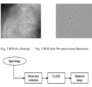
The mammogram image for this study is taken from Mammography Image Analysis Society (MIAS)†, which is an UK research group organization related to the Breast cancer investigation [13]. As mammograms are difficult to interpret, preprocessing is necessary to improve the quality of image and make the feature extraction phase as an easier and reliable one. The calcification cluster/tumor is surrounded by breast tissue that masks the calcifications preventing accurate detection and shown in Figure.3. .A pre-processing; usually noise-reducing step [14] is applied to improve image and calcification contrast figure 3. In this work the efficient filter (CLAHE) was applied to the image that maintained calcifications while suppressing unimportant image features. Figures 3 shows representative output image of the filter for a image cluster in figure 2. By comparing the two images, we observe background mammography structures are removed while calcifications are preserved. This simplifies the further tumor detection step.
Fig. 2 ROI of a Benign Fig. 3 ROI after Pre-processing Operation
Fig.4. Image pre-processing block diagram.
2.3. Histogram Equalization
Histogram equalization is a method in image processing of contrast adjustment using the image's histogram [17]. Through this adjustment, the intensities can be better distributed on the histogram. This allows for areas of lower local contrast to get better contrast. Histogram equalization accomplishes this by efficiently spreading out the most frequent intensity values. The method is useful in images with backgrounds and foregrounds that are both bright or both dark. In particular, the method can lead to better views of bone structure in x-ray images, and to better detail in photographs that are over or under-exposed. In mammogram images Histogram equalization is used to make contrast adjustment so that the image abnormalities will be better visible.
†
peipa.essex.ac.uk/info/mias.html .
3. Feature extraction
Features, characteristics of the objects of interest, if selected carefully are representative of the maximum relevant information that the image has to offer for a complete characterization a lesion [18, 19]. Feature extraction methodologies analyze objects and images to extract the most prominent features that are representative of the various classes of objects. Features are used as inputs to classifiers that assign them to the class that they represent.
In this Work intensity histogram features and Gray Level Co-Occurrence Matrix (GLCM) features are extracted.
3.1 Intensity Histogram Features
Intensity Histogram analysis has been extensively researched in the initial stages of development of this algorithm [18,20]. Prior studies have yielded the intensity histogram features like mean, variance, entropy etc. These are summarized in Table 1 Mean values characterize individual calcifications; Standard Deviations (SD) characterize the cluster. Table 2 summarizes the values for those features.
Table 1: Intensity histogram features
Feature Number assigned Feature
1. Mean
2. Variance
3. Skewness
4. Kurtosis
5. Entropy
6. Energy
In this paper, the value obtained from our work for different type of image is given as follows
Table 2: Intensity histogram features and their values
Imag e Type
Features
Mea n
Varia nce
Skewne ss
Kurtos is
Entro py
En erg y norma
l
7.25 34
1.690 9
-1.4745 7.8097 0.250 4
1.5 152 malig
nant 6.81 75
4.098 1
-1.3672 4.7321 0.190 4
1.5 555 benig
n
5.62 79
3.183 0
-1.4769 4.9638 0.268 2
1.5 690
3.2 GLCM Features
Each element (I, J) in the resultant GLCM is simply the sum of the number of times that the pixel with value I
occurred in the specified spatial relationship to a pixel with value J in the input image.
3.2.1 GLCM Construction
GLCM is a matrix S that contains the relative frequencies with two pixels: one with gray level value i and the other with gray level j-separated by distance d at a certain angle θ occurring in the image. Given an image window W(x, y, c), for each discrete values of d and θ, the GLCM matrix S(i, j, d, θ) is defined as follows.
An entry in the matrix S gives the number of times that gray level i is oriented with respect to gray level j such that W(x
1, y1)=i and W(x2, y2)=j, then
We use two different distances d={1, 2} and three different angles θ={0°, 45°, 90°}. Here, angle representation is taken in clock wise direction.
Example
Intensity matrix
The Following GLCM features were extracted in our research work:
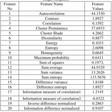
Autocorrelation, Contrast, Correlation, Cluster Prominence, Cluster Shade, Dissimilarity Energy, Entropy, Homogeneity, Maximum probability, Sum of squares, Sum average, Sum variance, Sum entropy, Difference variance, Difference entropy, information measure of correlation1, information measure of correlation2, Inverse difference normalized. Information difference normalized. The value obtained for the above features from our work for a typical image is given in the following table 3.
..
Table 3 : GLCM Features and values Extracted from Mammogram Image(Malignant)
Feature No
Feature Name Feature
Values
1 Autocorrelation 44.1530
2 Contrast 1.8927
3 Correlation 0.1592
4 Cluster Prominence 37.6933
5 Cluster Shade 4.2662
6 Dissimilarity 0.8877
7 Energy 0.1033
8 Entropy 2.6098
9 Homogeneity 0.6645
10 Maximum probability 0.6411
11 Sum of squares 0.1973,
12 Sum average 44.9329
13 Sum variance 13.2626
14 Sum entropy 133.5676
15 Difference variance 1.8188
16 Difference entropy 1.8927
17 Information measure of correlation1 1.2145
18 Information measure of correlation2 -0.0322 19 Inverse difference normalized 0.2863 20 Information difference normalized 0.9107
4. Feature subset selection
Feature subset selection helps to reduce the feature space which improves the prediction accuracy and minimizes the computation time [23]. This is achieved by removing irrelevant, redundant and noisy features .i.e., it selects the subset of features that can achieve the best performance in terms of accuracy and computation time. It performs the Dimensionality reduction.
Features are generally selected by search procedures. A number of search procedures have been proposed. Popularly used feature selection algorithms are Sequential forward Selection, Sequential Backward Selection, Genetic Algorithm and Particle Swarm Optimization, Branch and Bound feature optimization. In this work a new approach of oscillating search for feature selection technique [24] is proposed to select the optimal features. The selected optimal features are considered for classification. The oscillating search has been fully exploited to select the feature from mammogram which is one of the best techniques to optimize the features among many features. We have attempted to optimize the feature of GLSM and statistical features.
4.1 Oscillating Search Algorithms for Feature
Selection
known subset selection methods the oscillating search is not dependent on pre-specified direction of search (forward or backward). The generality of oscillating search concept allowed us to define several different algorithms suitable for different purposes. We can specify the need to obtain good results in very short time, or let the algorithm search more thoroughly to obtain near-optimum results. In many cases the oscillating search over-performed all the other tested methods. The oscillating search may be restricted by a preset time-limit, what makes it usable in real-time systems.
Note that most of known suboptimal strategies are based on step-wise adding of features to initially empty features set, or step-wise removing features from the initial set of all features, Y. One of search directions, forward or
backward, is usually preferred, depending on several factors [25], the expected difference between the original and the final required cardinality being the most important one. Regardless of the direction, it is apparent, that all these algorithms spend a lot of time testing features subsets having cardinalities far distant from the required cardinality d.
Before describing the principle of oscillating search, let us introduce the following notion: the “worst” features o- tuple in Xd should be ideally such a set , that
The “best” feature o-tuple for Xd should be ideally such a set , that
In practice we allow also suboptimal finding of the “worst” and “best” o-tuples to save the computational time (see later).
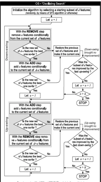
4.1.1. Oscillating Search
Unlike other methods, the oscillating search (OS) is based on repeated modification of the current subset Xd of d
features. This is achieved by alternating the down- and up-swings. The down-swing removes o “worst” features from the current set Xd to obtain a new set Xd-o at first, then adds
o “best” ones to Xd-o to obtain a new current set Xd . The
up-swing adds o “good” features to the current set Xd to obtain a new set Xd+o at first, then removes o “bad” ones from Xd+o to obtain a new current set Xd again. Let us denote two successive opposite swings as an oscillation cycle. Using this notion, the oscillating search consists of repeating oscillation cycles. The value of o will be denoted
oscillation cycle depth and should be set to 1 initially. If the last oscillation cycle did not find better subset Xd of d features, the algorithm increases the oscillation cycle depth by letting o = o+1. Whenever any swing finds better subset Xd of d features, the depth value o is restored to 1. The algorithm stops, when the value of o exceeds the
user-specified limit ∆. The course of oscillating search is illustrated on picture 1.
Every oscillation algorithm assumes the existence of some initial set of d features. Obtaining such an initial set will be denoted as an initialization. Oscillating algorithms may be initialized in different ways; the simplest ways are random selection or the SFS procedure. From this point of view the oscillating search may serve as a mechanism for tuning solution obtained in another way.
Whenever a feature o- tuple is to be added (or removed) from the current subset in the till now known methods, one of two approaches is usually utilized: the generalized
adding (or moving) find s the optimum o-tuple by means of exhaustive search (e.g. in GSFS, GSBS) or the
successive adding (or removing) single features o-time ( e.g. in basic Plus-l Minus-r), which may fail to find the optimum o- tuple, but is significantly faster.
In fact, we may consider finding feature o-tuples to be equivalent to the feature selection problem, though at a “Second level”. Therefore, we may use any search strategy for findings feature o-tuples. Because of proved effectiveness of floating search strategies we adopted the floating search principle as the third approach to adding (or removing) feature o-tuples in oscillating search. Note that in such a way one basic idea has resulted in defining a couple of new algorithms, as shown in the sequel.
For the sake of simplicity, let us denote the adding of feature o-tuple by ADD(o) and the removing of feature o-tuple by REMOVE(o). Finally, we introduce three versions of oscillating algorithm.
1. Sequential oscillating search : ADD (o) represents a sequention of o successive SFS steps (see [1]), REMOVE(o) represents a sequention of
o successive SBS steps.
2. Floating oscillating search : ADD (o) represents adding of o features by means of the SFFS procedure (see [5]), REMOVE (o) represents removing of o features by means of the SFBS procedure.
3. Generalized oscillating search : ADD (o) represents adding of o features by means by means of the GSFS(o) represents removing of o
features by means of the GSFS (o) procedure.
Remark : c serves as a swing counter.
Step 1 : Initialization: by means of the SFS procedure (or otherwise) find the initial set Xd of d features. Let
c = 0, Let o = 1.
not the so far best one among subsets having cardinality d-o, stop the down-swing and go to Step 3 *). By means of the ADD(o) step add the “best” feature o-tuple from Y\Xd-o to Xd-o to form a new subset X1d. If the J(X1d ) value is the so far best one among subsets having required cardinality d, let Xd = X1d, c= 0 and o = 1 and got Step 4.
Step 3 : Last swing did not find better solution.
Let c = c + 1. If c =2, the none of previous two swings has found better solution; extend the search, by letting o = o +1. If o > ∆, stop the algorithm, otherwise let c = 0.
Step 4 : Up-swing : By means of the ADD(o) step add the “best” feature o-tuple from Y \ Xd to Xd to form a new set Xd+0 (* If the J (Xd+o) value is not the so-far best one among subsets having cardinality
d+o, stop th up-swing and go to Step 5. *). “Worst” feature o-tuple from Xd+o to from a new set X1d . If the J (X1d) value is the so far best one among subsets having required cardinality d, let
Xd = X1d c=0 and o=1 and go to Step 2.
Step 5 : Last swing did not find better solution :
Let c =c+1. If c =2, the none of previous two swings has found better solution; extend the search by letting o = o +1, If o > ∆, stop the algorithm, otherwise let c = 0 and go to Step 2
---Remark : Parts of code enclosed in (* and *) brackets may be omitted to obtain a bit slower, more through procedure.
The algorithm is described also by a float chart on picture 2. The three introduced algorithm versions differ in their effectiveness and time complexity. The generalized oscillating search give the best results, but its use is restricted due to the time of complexity of generalized steps (especially for higher ∆). The floating oscillating search is suitable for findings solutions as close to optimum as possible in a reasonable time even in high-dimensional problems. The sequential oscillating search is the fastest but possibly the least effective algorithm versions with respect to approaching the optimal solution.
Fig.5. Simplified OS algorithm flowchart
By applying the proposed algorithm, it will produce a feature set contain best set of features which is less than the original set. This method will be providing a better and concrete relevant feature selection from 26 nos. of features to minimize the classification time and error and productive results in conjunction with better accuracy positively. The features selected by the method are given in table 4.
Table 4. Feature selected by proposed method
S.no. Features
1 Cluster prominence
2 Energy
3 Information measure of correlation 4 Inverse difference Normalized
6 Kurtosis
7 Contrast
8 Mean
9 Variance
10 Homogeneity
11 Entropy
5. Classification
5.1 Preparation of Transactional Database:
The selected features are organized in a database in the form of transactions [26], which in turn constitute the input for deriving association rules. The transactions are of the form[Image ID, F1; F2; :::; F9] where F1:::F9] are
9features extracted for a given image.
5.2 Association Rule Mining:
Discovering frequent item sets is the key process in association rule mining.
In order to perform data mining association rule algorithm, numerical attributes should be discretized first, i.e. continuous attribute values should be divided into multiple segments. Traditional association rule algorithms adopt an iterative method to discovery, which requires very large calculations and a complicated transaction process. Because of this, a new association rule algorithm is proposed in this paper. This new algorithm adopts a Boolean vector method to discovering frequent item sets. In general, the new association rule algorithm consists of four phases as follows:
1. Transforming the transaction database into the Boolean matrix.
2. Generating the set of frequent 1-itemsets L1. 3. Pruning the Boolean matrix.
4. Generating the set of frequent k-item sets Lk(k>1). The detailed algorithm, phase by phase, is presented below:
1. Transforming the transaction database into the Boolean matrix: The mined transaction database is D, with D
having m transactions and n items. Let T={T1,T2,…,Tm} be the set of transactions and I={I1,I2,…,In}be the set of items. We set up a Boolean matrix Am*n, which has m rows and n columns. Scanning the transaction database D, we use a binning procedure to convert each real valued feature into a set of binary features. The 0 to 1 range for each feature is uniformly divided into k bins, and each of k
binary features record whether the feature lies within corresponding range.
2. Generating the set of frequent 1-itemset L1: The Boolean matrix Am*n is scanned and support numbers of all items are computed. The support number Ij.supth of item Ij is the number of ‘1s’ in the jth column of the Boolean matrix Am*n. If Ij.supth is smaller than the minimum support number, itemset {Ij} is not a frequent 1-itemset and the jth column of the Boolean matrix Am*n will be deleted from Am*n. Otherwise itemset {Ij} is the frequent itemset and is added to the set of frequent 1-itemset L1. The sum of the element values of each row is recomputed, and the rows whose sum of element values is smaller than 2 are deleted from this matrix.
3. Pruning the Boolean matrix: Pruning the Boolean matrix means deleting some rows and columns from it. First, the column of the Boolean matrix is pruned according to Proposition 2. This is described in detail as: Let I• be the set of all items in the frequent set LK-1, where k>2. Compute all |LK-1(j)| where j belongs to I2, and delete the column of correspondence item j if |LK – 1(j)| is smaller than k – 1. Second, re-compute the sum of the element values in each row in the Boolean matrix. The rows of the Boolean matrix whose sum of element values is smaller than k are deleted from this matrix.
4. Generating the set of frequent k-itemsets Lk: Frequent k-item sets are discovered only by “and” relational calculus, which is carried out for the k-vectors combination. If the Boolean matrix Ap*q has q columns where 2 < q £ n and minsupth £ p £ m, k q c, combinations of k-vectors will be produced. The ‘and’ relational calculus is for each combination of k-vectors. If the sum of element values in the “and” calculation result is not smaller than the minimum support number minsupth, the k-itemsets corresponding to this combination of kvectors are the frequent itemsets and are added to the set of frequent k-itemsets Lk.
6. Experimental results
Table 5: Results obtained by proposed method
Normal 100%
Malignant 92.78%
Benign 100%
The confusion matrix has been obtained from the testing part .In this case for example out of 97 actual malignant images 07 images was classified as normal. In case of benign and normal all images are correctly classified. The confusion matrix is given in Table 6
. Table 6: Confusion matrix
Actual Predicted class
Benign Malignant Normal
Benign 104 0 0
Malignant 97 90 07
Normal 99 0 99
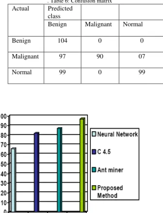
Fig. 5. Performance of the Classifier
7. Conclusion
Automated breast cancer detection has been studied for more than two decades Mammography is one of the best methods in breast cancer detection, but in some cases radiologists face difficulty in directing the tumors. We have described a comprehensive of methods in a uniform terminology, to define general properties and requirements of local techniques, to enable the readers to select the efficient method that is optimal for the specific application in detection of micro calcifications in mammogram images. In this paper, a new method for association rule mining is proposed. The main features of this method are that it only scans the transaction database once, it does not
produce candidate jtemsets, and it adopts the Boolean vector “relational calculus” to discover frequent itemsets. In addition, it stores all transaction data in binary form, so it needs less memory space and can be applied to mining large databases.
The CAD mammography systems for micro calcifications detection have gone from crude tools in the research laboratory to commercial systems. Mammogram image analysis society database is standard test set but defining different standard test set (database) and better evaluation criteria are still very important. With some rigorous evaluations, and objective and fair comparison could determine the relative merit of competing algorithms and facilitate the development of better and robust systems. The methods like one presented in this paper could assist the medical staff and improve the accuracy of detection. Our method can reduce the computation cost of mammogram image analysis and can be applied to other image analysis applications. The algorithm uses simple statistical techniques in collaboration to develop a novel feature selection technique for medical image analysis.
Appendix
Appendixes, if needed, appear before the acknowledgment.
References
[1]. Majid AS, de Paredes ES, Doherty RD, Sharma N Salvador X. “Missed breast carcinoma: pitfalls and Pearls”. Radiographics, pp.881-895, 2003.
[2]. Osmar R. Zaïane,M-L. Antonie, A. Coman “Mammography Classification by Association Rule based Classifier,” MDM/KDD2002 International Workshop on Multimedia Data Mining ACM SIGKDD, pp.62-69,2002,
[3]. Xie Xuanyang, Gong Yuchang, Wan Shouhong, Li Xi ,”Computer Aided Detection of SARS Based on Radiographs Data Mining “, Proceedings of the 2005 IEEE Engineering in Medicine and Biology 27th Annual Conference Shanghai, China, pp7459 – 7462, 2005.
[4] C.Chen and G.Lee, “Image segmentation using multitiresolution wavelet analysis and Expectation Maximum(EM) algorithm for mammography” , International Journal of Imaging System and Technology, 8(5): pp491-504,1997.
[5] T.Wang and N.Karayaiannis, “Detection of microcalcification in digital mammograms using wavelets”, IEEE Trans. Medical Imaging, 17(4):498-509, 1998.
mammography”Grgic et al. (Eds.): Rec. Advan. in Mult. Sig. Process. and Commun., SCI 231, pp. 631–657,2009
[7]. Shuyan Wang, Mingquan Zhou and Guohua Geng, “Application of Fuzzy Cluster analysis for Medical Image Data Mining” Proceedings of the IEEE International Conference on Mechatronics & Automation Niagara Falls, Canada,pp. 36 – 41,July 2005.
[8]. R.Jensen, Qiang Shen, “Semantics Preserving Dimensionality Reduction: Rough and Fuzzy-Rough Based Approaches”, IEEE Transactions on Knowledge and Data Engineering, pp. 1457-1471, 2004.
[9]. I.Christiyanni et al ., “Fast detection of masses in computer aided mammography”, IEEE Signal processing Magazine, pp:54- 64,2000.
[10]. Walid Erray, and Hakim Hacid, “A New Cost Sensitive Decision Tree Method Application for Mammograms Classification” IJCSNS International Journal of Computer Science and Network Security, pp. 130-138, 2006.
[11]. Ying Liu, Dengsheng Zhang, Guojun Lu, Regionbased “image retrieval with high-level semantics using decision tree learning”, Pattern Recognition, 41, pp. 2554 – 2570, 2008.
[12]. Kemal Polat , Salih Gu¨nes, “A novel hybrid intelligent method based on C4.5 decision tree classifier and one-against-all approach for multi-class classification problems”, Expert Systems with Applications, Volume 36 Issue 2,
pp.1587-1592, March, 2009, doi:10.1016/j.eswa.2007.11.051
[13]. Etta D. Pisano, Elodia B. Cole Bradley, M. Hemminger, Martin J. Yaffe, Stephen R. Aylward, Andrew D. A. Maidment, R. Eugene Johnston, Mark B. Williams,Loren T. Niklason, Emily F. Conant, Laurie L. Fajardo,Daniel B. Kopans, Marylee E. Brown, Stephen M. Pizer “Image Processing Algorithms for Digital Mammography: A Pictorial Essay” journal of Radio Graphics Volume 20,Number 5,sept.2000
[14] Pisano ED, Gatsonis C, Hendrick E et al. “Diagnostic performance of digital versus film mammography for breast-cancer screening”. NEngl J Med 2005; 353(17):1773-83. [15] Wanga X, Wong BS, Guan TC. ‘Image enhancement for
radiography inspection”. International Conference on Experimental Mechanics. 2004: 462-8.
[16]. D.Brazokovic and M.Nescovic, “Mammogram screening using multisolution based image segmentation”, International journal of pattern recognition and Artificial Intelligence, 7(6): pp.1437-1460, 1993
[17]. Dougherty J, Kohavi R, Sahami M. “Supervised and unsupervised discretization of continuous features”. In: Proceedings of the 12th international conference on machine learning.San Francisco:Morgan Kaufmann; pp 194–202, 1995.
[18]. Yvan Saeys, Thomas Abeel, Yves Van de Peer “Towards robust feature selection techniques”, www.bioinformatics.psb.ugent
[19] Gianluca Bontempi, Benjamin Haibe-Kains “Feature selection methods for mining bioinformatics data”, http://www.ulb.ac.be/di/mlg
[20]. Li Liu, Jian Wang and Kai He “Breast density classification using histogram moments of multiple resolution mammograms” Biomedical Engineering and Informatics (BMEI), 3rd International Conference, IEEE explore pp.146–149, DOI: November 2010, 10.1109/ BMEI.2010 .5639662,
[21]. Li Ke,Nannan Mu,Yan Kang Mass computer-aided diagnosis method in mammogram based on texture features, Biomedical Engineering and Informatics (BMEI), 3rd International Conference, IEEE Explore, pp.146 – 149, November 2010, DOI: 10.1109/ BMEI.2010.5639662, [22] Azlindawaty Mohd Khuzi, R. Besar and W. M. D. Wan
Zaki “Texture Features Selection for Masses Detection In Digital Mammogram” 4th Kuala Lumpur International Conference on Biomedical Engineering 2008 IFMBE Proceedings, 2008, Volume 21, Part 3, Part 8, 629-632, DOI: 10.1007/978-3-540-69139-6_157
[23] S.Lai,X.Li and W.Bischof “On techniques for detecting circumscribed masses in mammograms”, IEEE Trans on Medical Imaging , 8(4): pp. 377-386,1989.
[24]. Somol, P.Novovicova, J..Grim, J., Pudil, P.” Dynamic Oscillating Search Algorithm for Feature Selection” 19th International Conference on Pattern Recognition, 2008. ICPR 2008. pp.1-4 D.O.I10.1109/ICPR.2008.4761773
[25]. R. Kohavi and G. H. John. “Wrappers for feature subset selection”. Artif. Intell., 97(1-2):273–324, 1997.
[26] Deepa S. Deshpande “ASSOCIATION RULE MINING BASED ON IMAGE CONTENT” International Journal of Information Technology and Knowledge Management January-June 2011, Volume 4, No. 1, pp. 143-146
[27].Holmes, G., Donkin, A., Witten, I.H.: WEKA: a machine learning workbench. In: Proceedings Second Australia and New Zealand Conference on Intelligent Information Systems, Brisbane, Australia, pp. 357-361, 1994.
First Author: Aswini kumar mohanty has obtained his Bachelor of
engineering in computer technology in 1991 from Mararthawada University in 1991 and M.Tech. in computer science from kalinga university in 2005.Currently he is pursuing his phd under SOA university in image mining.He has served in many engineering colleges and presently working as Associate professor in computer science department of Gandhi Engineering college, Bhubaneswar, odhisa, His area of interest is Computer Architecture, Operating system, Data mining, image mining. He has published more than 15 papers in national and international conferences and journals.
degree in computer application (MCA) from Indira Gandghi Open University(IGNOU) in 2006 and currently pursuing his M.Tech degree in Computer Science under BPUT, Rourkela, Odisha and working as assistant professor in NIIS institute of Business Administration, Bhubaneswar, Odisha..
Third Author Pratap Kumar Champati obtained his bachelor of
engineering in computer science in 1993 from Utkal University and has worked in industries as well as in academics. Currently he is working as assistant professor in ABIT engineering college, cuttack, Orissa and also pursuing M.Tech. in computer science under BPUT, Rourkela, Odhisa.
Fourth Author Dr. Saroj kumar lenka Passed his B.E. CSE in
1994 from Utkal Universty and M.tech in 2005.He obtained his PHDfrom Berhampur University in 2008 from deptt of comp. sc.Currently he is working as a professor in deptt. of CSE at MODI University, Rajstan. His area of research is image processing, data mining and computer architecture.