Universidade Federal de Minas Gerais Instituto de Ciˆencias Exatas Curso de P´os-gradua¸c˜ao em Estat´ıstica
Juliana Freitas de Mello e Silva
Modelo Exponencial por Partes para Dados de Sobrevivˆencia
com Longa Dura¸c˜ao
Piecewise Exponential Model for Long Term Survival Data
Juliana Freitas de Mello e Silva
Modelo Exponencial por Partes para Dados de Sobrevivˆencia
com Longa Dura¸c˜ao
Piecewise Exponential Model for Long Term Survival Data
Disserta¸c˜ao apresentada ao Curso de Estat´ıstica da UFMG, como requisito para a obten¸c˜ao do grau de MESTRE em Estat´ıstica.
Orientador: F´abio Nogueira Demarqui
Doutor em Estat´ıstica
Co-orientador: Thiago Rezende dos Santos
Doutor em Estat´ıstica
Freitas de Mello e Silva, Juliana
Modelo Exponencial por Partes para Dados de Sobrevivˆencia com Longa Dura¸c˜ao / Juliana Freitas de Mello e Silva - 2016
73.p
1.Estat´ıstica. I.T´ıtulo.
Juliana Freitas de Mello e Silva
Modelo Exponencial por Partes para Dados de Sobrevivˆencia
com Longa Dura¸c˜ao
Piecewise Exponential Model for Long Term Survival Data
Disserta¸c˜ao apresentada ao Curso de Estat´ıstica da UFMG, como requisito para a obten¸c˜ao do grau de MESTRE em Estat´ıstica.
Aprovado em 22/02/2016.
BANCA EXAMINADORA
F´abio Nogueira Demarqui Doutor em Estat´ıstica
Thiago Rezende dos Santos Doutor em Estat´ıstica
Wagner Barreto de Souza Doutor em Estat´ıstica
`
Resumo
O Modelo Exponencial por Partes (MEP) ´e um modelo bastante utilizado, principalmente em an´alise de sobrevivˆencia. Ao utilizar esse modelo, uma parti¸c˜ao do eixo do tempo em um n´umero finito de intervalos ´e estabelecida e, em seguida, uma taxa de falha constante ´e considerada para cada um dos intervalos. Portanto, o MEP aproxima uma fun¸c˜ao cont´ınua, a saber a taxa de falha, atrav´es de seguimentos de reta. Por essa raz˜ao, o MEP ´e um modelo bastante flex´ıvel e, embora este seja um modelo param´etrico, ´e frequentemente considerado como n˜ao param´etrico. O presente trabalho prop˜oe uma abordagem bayesiana dinˆamica que permite a obten¸c˜ao de uma distribui¸c˜ao suavizada exata para os parˆametros representando a taxa de falha. Al´em disso a parti¸c˜ao do eixo do tempo (e, consequentemente, o n´umero de intervalos) ser´a considerada como uma quantidade desconhecida a ser estimada. Toda a abordagem proposta ser´a utilizada para modelar a fra¸c˜ao de cura em uma popula¸c˜ao, o que ocorre quando uma parte dos indiv´ıduos em um estudo ´e considerada curada e, portanto, nunca experimentar´a o evento de interesse. Para que seja poss´ıvel uma compara¸c˜ao, o caso com grade fixa tamb´em ser´a considerado. Por fim, ser´a mostrada uma aplica¸c˜ao a fim de ilustrar os conceitos apresentados.
Abstract
The Piecewise Exponential Model (PEM) is a very utilized model, mainly in survival analysis. When using this model, one considers a partition of the time axis into a finite number of intervals and, after that, a constant failure rate is considered to each interval. Therefore the PEM approximates a continuous function, the failure rate, through line segments. For this reason, the PEM is a very flexible model and, although it is a parametric model, it is often considered as non parametric one. The present work proposes a Bayesian dynamic approach that allows one to obtain the exact smoothed distribution for the parameters representing the failure rate. Moreover, the partition of the time grid (and, consequently, the number of intervals), will be considered as an unknown quantity to be estimated. This entire approach will be used to model the cure fraction in a population, which occurs when a part of the individuals in a study is considered cured and, therefore, will never experience the event of interest. For comparison purposes, the fixed time grid will also be considered. Lastly, in order to illustrate this approach, an application will be shown.
Agradecimentos
Come¸co meus agradecimentos com a frase “Yeah, I’m a lucky man, to count on both hands the ones I love. Some folks they’ve got one, yeah, others, they’ve got none.”. Ela me lembra do quanto devemos ser gratos sermos por quem somos, por quem nos cerca e pelo que possu´ımos, seja muito ou pouco.
Gostaria de agradecer `a minha fam´ılia. Principalmente `a minha mama Isabel, por ter me apoiado nessa parte t˜ao importante na minha vida. Pelo incentivo de sair de casa e (v)ir para BH, por aturar meus chororˆos de nervosismo ao telefone (e pessoalmente :D). Agrade¸co tamb´em `a minha tia C´assia pela for¸ca a aprova¸c˜ao que s˜ao t˜ao importantes pra mim. Agrade¸co aos meus irm˜aos Filipe, Mateus e Tiago e ao meu pai Geraldo.
`
A minha amiga de tanto tempo Isabella por estar sempre perto de mim, mesmo de longe. `A Juliana pela amizade e por compartilhar um pouco das minhas loucuras. Ao amigo Lucas por ser capaz de sempre colocar um sorriso no meu rosto, obrigada :). `A Jordana por se importar comigo e me ouvir.
Agrade¸co aos amigos que fiz durante a gradua¸c˜ao na UFF. Ao Bruno, pela amizade, pelo apoio, pelas conversas e por estar sempre presente. `A Fernanda eu agrade¸co por todas as visitas, sejam elas em Minas ou no Rio (quero mais visitas!). `A Carol e a Keilane pela amizade que continua, mesmo nos encontrando t˜ao pouco. Vocˆes s˜ao muito importantes pra mim!
Agrade¸co imensamente aos membros da Liga Externa: `a querida Caroline Ponce (e sua fam´ılia!), ao Luiz Fernando e ao Rafael Erbisti. Realmente sou agradecida pela paciˆencia e preocupa¸c˜ao que tiveram comigo, pela troca de conhecimento, por toda a ajuda, incentivo e apoio. Ah, pelas pizzas de toda santa ter¸ca tamb´em! Foi muito bom e fundamental ter vocˆes junto comigo.
mestrado. Ao Douglas pela amizade, pelas risadas e por toda a ajuda fornecida. Ao Edson, Guilherme, Milton, Uriel e demais colegas pela companhia e pelo conhecimento. Agrade¸co tamb´em `a Rafaella, ao Cristiano e ao Z´e Luiz pelas conversas e pela companhia.
`
A Silvana pela gentileza, simpatia e troca de conhecimento. Com certeza esse mestrado foi uma festa com vocˆes.
Agrade¸co `a Rachel por ter me ensinado muito sobre a vida, pela companhia, pelas risadas e pelas discuss˜oes filos´oficas antes de dormir.
Ao Paulo, eu agrade¸co por toda ajuda! Por toda a troca de conhecimento que foi muito boa e muito importante, tanto na parte dos conceitos quanto na parte computacional. Agrade¸co tamb´em o incentivo e otimismo.
Agrade¸co `a professora Alexandra Schmidt por mostrar conceitos de forma t˜ao simples e com tanto entusiasmo. Por mostrar tamb´em a importˆancia de conceitos sociais, algo que normalmente ´e esquecido no dia a dia. Agrade¸co tamb´em pela conversa e apoio.
Sou grata ao F´abio Demarqui e ao Thiago Rezende por terem possibilitado o conhecimento de conceitos t˜ao interessantes atrav´es da oportunidade de trabalhar nesse projeto. Pelas reuni˜oes e pelo incentivo.
Agrade¸co aos professores Valetin Sisko e Leonardo Bastos pela solicitude ao me forneceram a carta de recomenda¸c˜ao. Ao professor Wagner Barreto pelo excelente curso de Probabilidade, consegui aprender conceitos de uma ´area que considero t˜ao complicada. Agrade¸co novamente ao Leonardo e ao Wagner por aceitarem o convite e fazerem parte da banca.
Agrade¸co tamb´em, de forma geral, `a todas as pessoas que passaram pela minha vida, que torceram por mim e que, de alguma forma, fizeram com que eu chegasse at´e aqui.
Por ´ultimo e realmente n˜ao menos importante, agrade¸co `a CAPES pelo aux´ılio financeiro que, sem o qual, eu n˜ao teria cursado esse mestrado.
The future is paved with better days.
Sum´
ario
Lista de Figuras 8
Lista de Tabelas 9
1 Introduction 10
1.1 Purposes . . . 13
2 Basic Concepts in Survival Analysis 14
2.1 Proportional Hazards Model . . . 16
2.2 Cure Fraction Models . . . 17
3 The Piecewise Exponential Model 25
3.1 Random Time Grid . . . 32
4 Applications 41
4.1 Brain Cancer Data . . . 42
4.2 Melanoma Data . . . 48
5 Conclusions and Future Works 58
Lista de Figuras
2.1 Comparison of the follow-up time and the median survival time for the uncured individuals. . . 18
3.1 Ilustration of the quantity tj. . . 26
3.2 Illustration of the intervals’ grouping scheme. . . 34
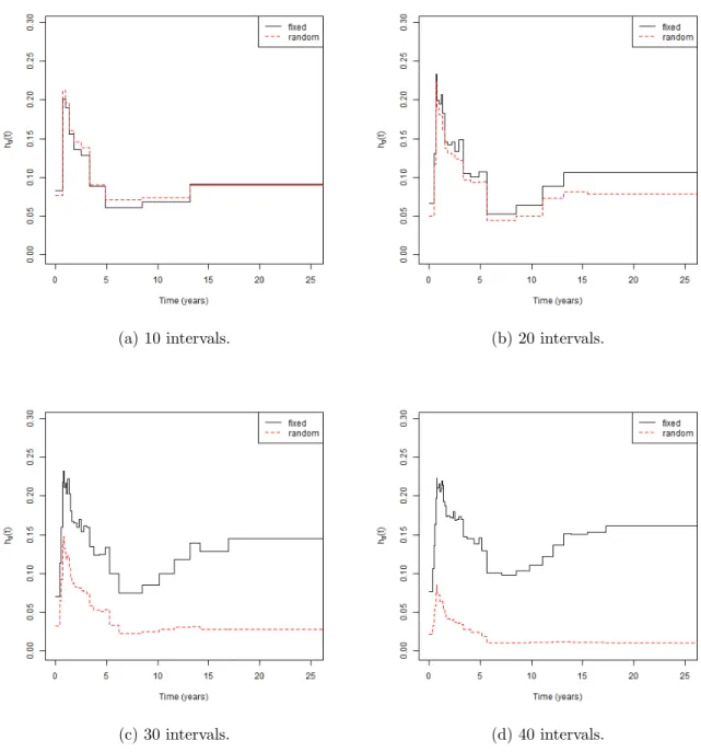
4.1 Comparison of the failure rate estimate varying the number of intervals. . . 43
4.2 Boxplot of the posterior discount factor sample for fixed and random time grid varying the (maximum) number of intervals. . . 44
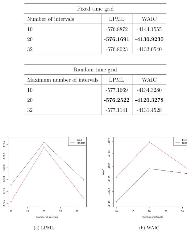
4.3 Model comparison measures for the fixed time grid x random time grid according to different (maximum) number of intervals. . . 45
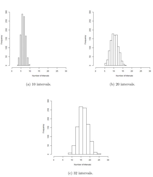
4.4 Histograms of the number of intervals varying the maximum number of intervals. . . 46
4.5 Estimated survival function. . . 47
4.6 Comparison of the failure rate estimates using fixed and random time grid and also varying the (maximum) number of intervals. . . 50
4.7 Model comparison measures for the fixed time grid x random time grid according to different (maximum) number of intervals. . . 51
4.8 Comparison of the probability of cure estimated varying the number of intervals. . . 52
4.9 Histogram of the number of intervals varying the maximum number of intervals. . . 53
4.10 Comparison of the discount factor estimates varying the number of intervals. 54
4.11 Comparison of the probability of cure separated by the covariates age and sex. . . 55
Lista de Tabelas
4.1 Comparison of fixed time grid x random time grid according to different (maximum) number of intervals. . . 45
4.2 Summary of the number of intervals. . . 46
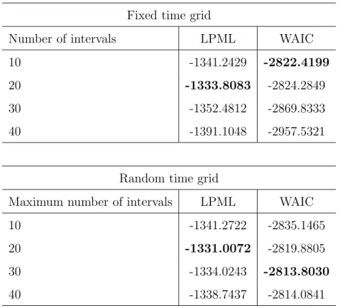
4.3 LPML and WAIC results. . . 49
4.4 Estimates of the intercept (ψ1) for the case with random time grid varying
the maximum number of intervals. . . 51
4.5 Summary of the number of intervals. . . 52
10
1 Introduction
Survival analysis is an area of statistics utilized when the intent is to study the time until the occurrence of an event of interest. Several studies involving survival analysis are concentrated in the medical area, but there are also important applications on engineering, economy, quality control, among others.
Survival data have intrinsic characteristics such as asymmetry and incomplete observations, called censure. Therefore, specific methods are required. One of the impor-tant quantities related to this area is the hazard function, or failure rate. This function provides the risk that the event of interest has to happen and it brings along with it a challenge: when modeling parametrically, the most utilized models impose a particular form, or few particular forms, for this function. For example, by choosing the Weibull or Gamma model it is possible to obtain an increasing, a decreasing or a constant hazard function. Other distributions, such as the Birnbaum-Saunders (Birnbaum and Saunders, 1969) and the Generalized Weibull are richer in form, however, the challenge still remains. It arises when the chosen model and the shapes that it carries are not the most suitable one to fit the data, thus this function would not be well represented.
A fine alternative to model survival data is the Piecewise Exponential Model (PEM). Basically, to define this model one has to partition the time axis into b intervals and to assume a constant failure rate in each interval. By using this model one is approxi-mating the failure rate by line segments. For this reason, the hazard function of the PEM does not have a pre-determinated form, providing great flexibility in the survival data modeling. Based on this characteristic, the PEM is often regarded as a nonparametric model, although in fact, it is a parametric one.
1 Introduction 11 The number of intervals must be chosen with caution: if it is too large there will be few data in each interval, leading to poor and/or unstable estimates; on the other hand, if it is too small, the true shape of the hazard function may not be achieved. A good number must balance the quantity of data in each interval, providing a good estimation for both hazard and survival functions (Demarqui, 2010). Alternatively, one can estimate the partition of the time axis and, consequently, the number of intervals. In most works found in the literature the time grid is chosen arbitrarily, fixing the number of intervals. Some of these works are: Gamerman (1991), Gamerman (1994), Ibrahim et al. (2001a), Yin and Ibrahim (2005), de Castro et al. (2009) and de Castro et al. (2015). However, there are also those who estimate it: Arjas and Gasbarra (1994), McKeague and Tighiouart (2000), Kim et al. (2007) and Demarqui (2010) estimate it through different approaches. Kim et al., for example, make use of Reversible Jump while on Demarqui’s work, the Product Partition Model (PPM) is used.
The estimation of the hazard function can be done by using different approa-ches within the Bayesian context: one can assume that the components of this function are independent; a dynamic model can be used, that is, it is possible to carry information along the intervals; historical data can also be used to construct the prior distribution (see Ibrahim et al. (2001b)).
Yin and Ibrahim (2005), for example, consider the components of the hazard function as independent a priori. Gamerman (1991) and Gamerman (1994) considers a dynamic approach to estimate the hazard function, which relates each component of the hazard function through an evolution equation. The difference between these two works relies on the evolution equation: in the first work, the author includes time-dependent covariates, making the hazard function to be a function that depends only on the (time dependent) coefficients and covariates; in the second one, however, there are no covaria-tes, thus the hazard function of an interval depends only on the hazard function of the previous one. de Castro et al. (2009) also considers the components of the hazard func-tion as dependent. In Demarqui (2010) there is a comparison of different types of prior distributions for the hazard function: independent Gamma prior, Jeffrey’s prior, prior within the dynamic approach and structural prior. In all works that used the dynamic model, an online and an approximated smoothed distribution were obtained.
1 Introduction 12 interest. By using such models it is possible to obtain information about the factors that influence the cured individuals as well as those factors related to the non-cured ones, separately; and also the probability of cure. Those information are very important to patients who suffer from cancer, for example.
There are two approaches concerning the cure fraction: the Mixture and the Promotion Time models. First, Boag (1949) and Berkson and Gage (1952) proposed the mixture cure rate model. In a brief way, this approach splits the population into two sub-populations: one is composed by the cured individuals and the other, by the non-cured ones. The Promotion Time Model, in turn, was introduced in 1996, by Yakovlev and Tsodikov based on a attractive biological motivation. Chen et al. (1999) extended this model for the Bayesian context. Ibrahim et al. (2001b) show an approach that allows the link between these two models.
There are several extensions and applications involving cure rate models: in Ibrahim et al. (2001a) the authors introduce a parameter to control the right tail of the survival curve, in a way that it becomes possible to control the degree of parametricity in the beginning, in the middle and, most importantly at the end of the survival distribution. Banerjee and Carlin (2004) use cure fraction model in the context of spatial analysis applied to a smoking cessation study. Yin and Ibrahim (2005) propose a cure fraction model that allows one to obtain zero and non zero cure fraction estimates, that is, there is no need to assume a cure fraction, the proposed model engages both cases. In Basu and Tiwari (2010) there is an extension involving competing risks and an interesting application involving breast cancer patients. In turn, Cucchetti et al. (2015) applied cure fraction model to study patients that suffered from colorectal liver metastases.
Nevertheless, in most works found in the literature (Kim et al. (2007), de Cas-tro et al. (2009), Demarqui et al. (2014) and others) the information from the covariates is used only to explain the cure fraction. It would be interesting to observe how these covariates influence the non-cured individuals as well.
1.1 Purposes 13 be considered and the information from covariates will be used to explain both cured and non-cured individuals.
This work is organized as follows. Chapter 2 explicits the basic theory in which this work is based on. The concepts showed in this Chapter will be essential for understanding this work. In Chapter 3 the Piecewise Exponential model is explored and discussed. In turn, in Chapter 4 two applications are presented with the aim to illustrate the concepts presented. At last, Chapter 5 concerns the conclusions obtained as well as the future works.
1.1
Purposes
The aim of this study is to consider the Piecewise Exponential Model in the Bayesian dynamic approach. In the present work the parameters representing the hazard function will be correlated so that the information of the previous interval can be used to estimated the actual one. By doing this, a quantity to control the passage of information is introduced. This quantity is called discount factor and it will be estimated, differently from most works in the literature. The evolution equation used in this work allows the achievement of an exact smoothed distribution, this is also commonly obtained in an estimated way.
The time grid of the PEM will be estimated via Product Partition Model and the results obtained will be compared to the fixed time grid case. In turn, the whole modeling procedure obtained will be used to study cure fraction models. These studies are standing out in the literature, since new and more effective treatments are emerging.
14
2 Basic Concepts in Survival Analysis
In this chapter, basic concepts and properties used in survival analysis will be introduced and discussed. These concepts will be essential for understanding this present work.
Survival analysis can be used when the interest is to study the time until the occurrence of a certain event. Let T be the non negative random variable representing the observed time. This time may be a failure time or a censured time. A failure time occurs when the event is fully observed, whereas a censored time takes place when the time to event is, for some reason, not fully observed due to, for instance, by the end of the study, the lost of follow-up, death of the patient for some other reason than that particular one of interest, among others (Colosimo and Giolo, 2006; Carvalho et al., 2011). Another typical characteristic found in survival data is asymmetry, which makes impracticable the usage of common methods, generally involving the Normal distribution.
There are three types of censoring, namely: left censoring, right censoring and interval censoring. Left censoring occurs when the event of interest has happened before the time to event is observed, for example, in a study where the event is the first time the individual has smoked a cigarette, the individual may not remember when it was, but it is known for sure that, if it happened, it happened before the interview; right censoring occurs when the actual time to event is known to be greater than the observed time; in turn, interval censoring occurs when it is known that the time to event has occurred in a interval, for example, when the study considers seropositive patients and the interest is to evaluate when the progression to AIDS will happen, it will be known that this time will be between two exams, but the exact time will be unknown.
2 Basic Concepts in Survival Analysis 15 An indicator variable, δi, will be used to represent whether the i−th time is
a failure or a censured time, that is:
δi =
1, if the failure occurred for thei−th individual , 0, if the i−th individual is right censored.
Therefore, for each individual the information will be the pair (ti, δi), where i
represents the i−th individual. If there is information from covariates, the information will be represented by (ti, δi,xi), wherexi is the covariates vector associated to the i−th
individual.
LetT be a continuous non-negative random variable whose probability density function (p.d.f.) is f(t). The survival function is defined as:
S(t) =P(T > t) = 1−F(t), t >0 . (2.1)
This function has the following well-known properties:
1. S(0) = 1;
2. lim
t→∞S(t) = 0;
3. S(t) is a decreasing function in t.
The first property means that at time 0, all the individuals have not suffered the event of interest (for example, if the event is death from breast cancer, all individuals have not died from this disease); the second property means that ast → ∞, all individuals will eventually suffer the event of interest.
The hazard function is defined as the instantaneous rate of failure at time t. Its expression is given by:
h(t) = lim
∆t→0
P(t < T ≤t+ ∆t|T > t)
∆t , t >0 . (2.2)
Another important function is the cumulative hazard function, which is given by
H(t) =
Z t
0
h(u)du,t >0 . (2.3)
2.1 Proportional Hazards Model 16
S(t) = exp
− Z t 0 h(u)du ,
f(t) =−d
dtS(t) ,
h(t) = d
dtlog(S(t)).
Also, note that:
f(t) = d
dtF(t) = d
dt[1−S(t)] =− d
dtS(t) =− d dtexp − Z t 0 h(u)du = − exp − Z t 0 h(u)du
(−h(t))
=S(t)h(t) . (2.4)
That is, f(t) = S(t)h(t) and then h(t) = f(t) S(t).
2.1
Proportional Hazards Model
One may think of including covariates into the model. In this case, a very important model is the proportional hazards (PH) model. This model was proposed by Cox (1972) and it includes the information from covariates through the hazard function, in the following way:
h(t|x) =h0(t) exp (xβ) , (2.5)
where h0(t) is the baseline hazard function, xis the covariates vector andβ is the vector
of regression coefficients.
This model has the property of proportional hazards, that is, the hazard ratio of two individuals does not depend on time. This property can be seen through Equation (2.6), where x1 and x2 are the covariates vector of two different individuals.
h(t|x1)
h(t|x2)
= h0(t) exp (x1β) h0(t) exp (x2β)
= exp (x1β) exp (x2β)
. (2.6)
2.2 Cure Fraction Models 17 mechanism, it is given by the p.d.f. for those individuals whose time to event is completely observed and the survival function for those whose time to event is (right) censored. That is:
L(Φ;D) =
n
Y
i=1
f(ti|Φ)δi(S(ti|Φ))1−δi = n
Y
i=1
h(ti|Φ)δiS(ti|Φ), (2.7)
where Φis the vector of parameters to be estimated which includes the vector of coeffici-ents. D represents the data available, in this case D= (ti, δi,xi), i= 1,2, . . . , n; n is the
number of individuals and, lastly, ti represents the time to event of the i−th individual.
2.2
Cure Fraction Models
Over the past decades, with the advance of medicine, patients’ survival is being improved and it implies directly on the probability of survival, usually raising it. For this reason, a considerable part of patients is being cured. It is important to highlight that the concept of “cure” is not strictly medical; in fact, if an individual is considered cured it means that the event will never happen to this specific individual. This characteristic violates the second property of the survival function, that is, the survival function does not go to 0 as t → ∞, it goes to the proportion of healed individuals, which will be represented by π∈[0,1].
Cure fraction models were developed to adapt these situations. In the literature there are several articles that analyze data with a cure fraction, such as Farewell (1982), Farewell (1986), Ibrahim et al. (2001a), Kim et al. (2007) and others.
The challenge, at this point, is to separate the truly cured individuals from those who have not suffered the event yet, due to the duration of the follow-up, for example. According to Yu et al. (2004), the efficiency of the estimate of the cure rate depends, among other factors, on the follow-up time. Cases in which the follow-up time is relatively greater than the median of the survival time for the uncured individuals are the cases in which the cure rate presents better estimates. This is due to the confusion between the truly cured individuals with those who just have not suffered the event of interest yet (but they would, if the follow-up time was long enough).
2.2 Cure Fraction Models 18 described in Ibrahim et al. (2001b), in which the event of interest is death from melanoma. The dotted red line represents the median survival time for the non-cured individuals. Note that the follow-up time is considerably larger than the median survival time.
Figure 2.1: Comparison of the follow-up time and the median survival time for the uncured individuals.
Moreover, Lambert (2007) points out that when using cure fraction models one is assuming that there is a cure, nevertheless it may not be medically correct. For example, studies in which the interest is to evaluate the time to death from a certain type of cancer but it is only recorded if the individuals had died or not, the cause of death in unknown; in this case one would be assuming that exits cure from death, which is senseless.
Therefore, to introduce this model, consider a non-negative functionf∗(t) such that
Z ∞
0
f∗(t)dt = 1 −π ≤ 1 and, given that, the adapted survival function, called improper survival function will be (Rodrigues et al., 2008):
Spop(t) =π+
Z ∞
t
f∗(u)du (2.8)
This function will have the following properties:
2.2 Cure Fraction Models 19 2. Spop(0) = 1;
3. Spop(t) is a decreasing function in t;
4. limt→∞Spop(t) =π.
The first property refers to the case when there’s no cure fraction, thus the analysis will be the same as the one presented before; therefore, S(t) is a genuine survival function. The meaning of the second and third properties is analogue to the proper survival function and, the fourth one means that whent → ∞, the survival function goes to the proportion of the cured individuals.
The most important cure fraction models found in the literature are the mix-ture and the promotion time models. These models carries advantages and disadvantages: the mixture model is quite logical and the promotion time model has an interesting bi-ological motivation that enriches the interpretation in a study. However, as pointed out by Rodrigues et al. (2008), the mixture model allows only one causing factor of the event of interest whereas the promotion time model allows more than one. Besides that, the assumption of proportional hazards may no longer be preserved, mainly for the mixture model (Ibrahim et al., 2001b; Rodrigues et al., 2009). According to Ibrahim et al. (2001b), this assumption is no longer attained for the mixture model when the probability of cure is modeled through a binomial regression.
Mixture Model
The mixture model was proposed by Boag (1949) and Berkson and Gage (1952) and it is given by:
Spop(t) = π+ (1−π)S(t). (2.9)
The idea of this model is to include the individuals through two components: one representing the cured individuals and the other representing the non-cured ones along with its survival. In this way π represents the proportion of cured individuals and, consequently, 1−π represents the non cured ones; S(t) is the usual (and proper) survival function for the non-cured individuals, that is, S(t) =
Z ∞
t
2.2 Cure Fraction Models 20 Consequently, the populational hazard function and the “p.d.f.” will be given by:
fpop(t) = −
d
dtSpop(t) = (1−π)f(t), (2.10) hpop(t) =
fpop(t)
Spop(t)
. (2.11)
Note that Equation (2.10) is not a proper p.d.f. indeed, because
Z ∞
0
fpop(t) =
(1−π)
Z ∞
0
f(t) = 1−π ≤1.
So, substituting Spop(t) and fpop(t) in Equation (2.7), the likelihood function
for n individuals will be given by:
L(Φ,ψ;D) =
n
Y
i=1
[(1−πi)f(ti|Φ)]δi[πi+ (1−πi)S(ti|Φ)]1−δi
=
n
Y
i=1
[(1−πi)S(ti|Φ)h(ti|Φ)]δi[πi+ (1−πi)S(ti|Φ)]1−δi, (2.12)
where Φ is the vector including the parameters that indexes f and the coefficients of the non-cured individuals. In turn, πi = g(ziψ) for some link function g(.), this link
function may be the logit, for example. The covariates associated to the cure fraction can be different from the ones used to model the non-cured individuals. Therefore to model the cure fraction, let zi represent the vector of covariates of the i−th individual and, consequently, ψ is the coefficients’ vector, including the intercept. Moreover, in this case, D= (ti, δi,xi,zi), for i= 1,2, . . . , n.
It is noteworthy, in the Bayesian context, that the prior distribution forψ, the vector of coefficients associated to the cure fraction, must be chosen carefully as improper priors may not lead to a proper posterior distributions (Ibrahim et al., 2001b). Moreover, few issues involving this model were found both in the literature and practice, such as convergence problems when using large variance for the cure fraction coefficients prior (Banerjee and Carlin, 2004) and identifiability problems (Klein et al., 2014).
2.2 Cure Fraction Models 21 model. Taylor (1995) and Peng (2003) describe solutions to this problem: in a very brief explanation these authors force the improper survival function to become a proper one.
Another discussion to justify the issues attached to the usage of the mixture model can be found in Klein et al. (2014). They point out the possible confusion obtained when using the same covariates to model the cure fraction and the non-cured individuals.
Therefore, taking these points into account, the focus will rely only on the promotion time model.
Promotion Time Model
The promotion time model was developed by Yakovlev and Tsodikov (1996) and its Bayesian version was proposed by Chen et al. (1999). This model has an interesting and appealing biological motivation: consider a scenario in which an individual that underwent a treatment due to a certain type of cancer. After this procedure there may remain some cancer cells that may become active again and develop a new tumor, in other words, the individual may relapse. Starting from this scenario, consider N as the number of competent cells, that is, those cells that can become a tumor, andZl,l= 1,2, . . . , N the
time until the l-th competent cell will become active, this time is also called the promotion time. One characteristic of this model is that the number of competent cells is a latent random variable and, given this, Zl, l = 1,2, . . . are considered to be independent and
identically distributed (i. i. d.), with a cumulative distribution function F(t), which does not depend on N. This distribution can be the Exponential or the Weibull, for example; in this present work it will be the Piecewise Exponential distribution.
The time to relapse is the time until the first competent cell becomes active, that is, T = min{Zl,0≤l ≤N}, with P(Z0 = ∞) = 1. In this way, if there is no
competent cell, the subject is considered cured and therefore, the time until a competent cell becomes active is, certainly, infinite.
2.2 Cure Fraction Models 22 first one to happen, is observed; for example, in a study where the interest is to evaluate the death from breast cancer but there are numerous cases of death from other causes, these two outcomes will be “competing” to each other until one of them occur (see more about competing risks in Carvalho et al. (2011) and Klein and Moeschberger (2003)).
For this model, the improper survival function is given by:
Spop(t) = P(no competent cell is active until time t)
= P(N = 0) +P([Z1 > t, Z2 > t, . . . , ZN > t]∩[N ≥1])
= P(N = 0) +P(Z1 > t, Z2 > t, . . . , ZN > t|N ≥1)P(N ≥1)
= P(N = 0) +
∞ X
n=1
P(N =n)(S(t))n, (2.13)
where S(t) is the proper survival function.
This improper survival function is the probability that no competent cell is active until time t because, if this happens it means that the individual has not relapsed or, in other words, the individual survived the relapse. This probability can be divided into two groups, one representing the cured (N = 0) individuals and the other, the non-cured ones (N ≥1). In the first case, there is no competent cell that may become active, thus it is given by the probability that N = 0; on the other case it will be given by the probability of each of the N, N ≥1, cells has not become active until time t.
As is it usually done (Chen et al., 1999; Sinha et al., 2003; Lambert and Thomp-son, 2007), in this work the latent random variable N will follow a P oisson distribution with mean θ. By doing so, it is possible to obtain that:
Spop(t) = exp{−θ}+
∞ X
k=1
S(t)kθ
kexp{−θ}
k!
= exp{−θF(t)}, (2.14)
where S(t) is the genuine survival function. Also, note thatSpop(∞) = exp{−θ} ∈(0,1).
2.2 Cure Fraction Models 23 The improper p.d.f. and hazard function can be easily obtained by using the relationships between these and the survival function:
fpop(t) = θf(t) exp{−θF(t)}, (2.15)
hpop(t) = θf(t). (2.16)
Other interesting and useful quantities are the survival, hazard and probability density functions for the non-cured individuals. They are given by:
SN C(t) = P(T > t|N ≥1) =
exp{−θF(t)} −exp{−θ}
1−exp{−θ} , (2.17)
fN C(t) =
exp{−θF(t)}
1−exp{−θ}
θf(t), (2.18)
hN C(t) =
exp{−θF(t)}
exp{−θF(t)} −exp−{θ}
hpop(t). (2.19)
Note that SN C(t) is a proper survival function because SN C(0) = 1 and
SN C(∞) = 0; consequently fN C(t) and hN C(t) are also proper. From these functions
it is possible to obtain an expression that links the mixture and the promotion time mo-dels. Thus, from one model it is possible to reach the other (more details in Ibrahim et al. (2001b)).
The likelihood function based on a sample of n individuals with all the infor-mation, that is, the observable and non-observable data, is given by:
L(Φ,ψ;D) =
n
Y
i=1
(S(ti|Φ))Ni−δi(Nif(ti|Φ))δi
! n Y
i=1
θNi
i exp{−θi}
Ni!
=
n
Y
i=1
(S(ti|Φ))Ni(Nih(ti|Φ))δi
! n Y
i=1
θNi
i exp{−θi}
Ni!
, (2.20)
where Φ is the vector of the parameters that indexes the p.d.f., which may include a vector of coefficients. Furthermore, analogously to the mixture model, the probability of cure can be modeled through covariates. In this case, a link function will be used, for example: θi = exp{ziψ}. Again, the covariates used to explain the cure fraction can be
different than the ones used to model the non-cure individuals, therefore, the entire data is composed by D = (ti, δi,xi,zi, Ni), i = 1,2, . . . , n, where xi represents the covariates
vector used to model the i−th non-cured individual and zi represents cure probability
for the same i−th individual.
As stated before, the probability of cure is given by the probability that the in-dividual has no competent cell: P(N = 0) = exp{−θ}= exp{−exp{zψ}} ≡ lim
t→∞Spop(t).
2.2 Cure Fraction Models 24 It is also possible to obtain a closed expression for the likelihood function based only on the observed data, Dobs = (ti, δi,xi,zi),i= 1,2, . . . , n. In this case, it is necessary
to sum out the latent variable N:
L(Φ,ψ;Dobs) =
X
N
L(Φ,ψ;D) =
n
Y
i=1
(θif(ti|Φ))δiexp{−θi(1−S(ti|Φ))} (2.21)
=
n
Y
i=1
(θih(ti|Φ)S(ti|Φ))δiexp{−θi(1−S(ti|Φ))}.
Lastly, in counterpart to the mixture model, the prior distribution of the coef-ficients for the cured fraction may be proper or improper; by using the Promotion Time model withNi ∼P oisson(θi), fori= 1,2, . . . , n, it is guaranteed that the posterior
25
3 The Piecewise Exponential Model
In this chapter, the Piecewise Exponential model (PEM) will be introduced. The aim is to discuss about this model’s properties and particularities, showing the advan-tages and the challenges that come along with it, motivating its usage and understanding. It will also be shown how to include covariates and incorporate the cure fraction.
The PEM was proposed by Kalbfleisch and Prentice (1973) and it has been very explored in the literature, mainly focusing on survival analysis.
In order to specify the PEM one has to, at first, consider a partition of the time axis. Thus, to divide the time axis in b intervals, let τ ={s0, s1, . . . , sb} represent
the cuts of the intervals, where 0 = s0 < s1 < · · · < sb < ∞. In that way the intervals
will be I1 = (s0, s1], I2 = (s1, s2], . . . , Ib = (sb−1, sb]. After that, a constant failure rate,
λj, for j = 1,2, . . . , b is assumed to each interval. So the hazard function is:
h(t) =λj, fort ∈Ij, j = 1,2, . . . , b. (3.1)
By using such model, one is approximating the hazard function, a continuous function, by line segments; therefore, this function does not have a predetermined shape and, in counterpart of the usual models such as Exponential, Weibull and Log-Normal, no shape must be imposed. This characteristic provides great flexibility for modeling the hazard function and for this reason, the PEM is often considered as a non-parametric model, although in fact, it is a parametric one.
Let T be a non-negative random variable representing the time to event. To introduce the cumulative hazard, consider tj, j = 1,2, . . . , b as:
tj =
sj−1, if t < sj−1 ,
t, if t∈(sj−1, sj] ,
sj, if t > sj .
(3.2)
For a better comprehension of the usefulness of the quantity tj, consider a
individual whose time to event is represented by Figure 3.1.
Assume that the time grid was divided in four intervals: I1 = (0, s1], I2 =
3 The Piecewise Exponential Model 26
Figure 3.1: Ilustration of the quantity tj.
event or the censorship at timet, that is, between s2 ands3. The hazard function (λ1,λ2,
λ3 and λ4) is the straight line segments and j represents thej−th interval. This time to
event is greater than the upper limit of the first interval (s1), that is t > s1, and therefore
t1 = s1 and this whole interval will be taken in consideration. The same is true for the
second interval, thereforet2 =s2. In turn, the time to event is lower than the upper limit
of the third interval (s3), this means that t ∈ (s2, s3], then t3 = t so that only a part of
it will be considered. Lastly, the time to event is lower than the lower limit of the fourth interval, so t4 =s3 and the fourth interval will not be taken in consideration.
Given this, the cumulative hazard function can be defined as:
H(t|λ) =
b
X
j=1
λj(tj−sj−1) , (3.3)
where λ= (λ1, λ2, . . . , λb) is the vector of failure rates.
One may visualize this hazard as the area of each interval. In the case of the Figure 3.1, it follows that
H(t|λ) =
4
X
j=1
λj(tj −sj−1) = λ1(t1−s0) +λ2(t2−s1) +λ3(t3 −s2) +λ4(t4−s3)
= λ1(s1−s0) +λ2(s2−s1) +λ3(t−s2) +λ4(s3 −s3)
3 The Piecewise Exponential Model 27 Using the relationship between the cumulative hazard function and the survival function, as well as the relationship between the survival function and the probability distribution function, described on page 16, it follows that:
S(t|λ) = exp
(
−
b
X
j=1
λj(tj −sj−1)
)
(3.4)
and
f(t|λ) =λjexp
(
−
b
X
j=1
λj(tj −sj−1)
)
, t∈Ij , λj >0, j = 1,2, . . . , b. (3.5)
An important discussion is about the number of intervals. This number can be fixed, as seen in Gamerman (1994), Yin and Ibrahim (2005), de Castro et al. (2009), among others. Nevertheless stipulating the number of intervals is a difficult task. If this number is too large, there will be few data in each interval, therefore it can result in poor and/or unstable estimates; on the other hand, if this number is too small, the hazard function may not be well approximated. Thus, the number of intervals should be carefully chosen, balancing the quantity of data in each interval so that it is possible to provide a good estimation for the hazard function and for the survival function as well. One way to solve this issue would be to estimate the time grid τ, that is, to consider the partition of the time axis and, consequently the number of intervals itself, as an unknown quantity to be estimated. In this work, in the same way as others (Kim et al., 2007; Demarqui, 2010) both cases will be considered. One restriction that may be done is to establish the maximum number of intervals as the number of distinct observed failures so that is guaranteed to exist at least one failure at each interval (Gamerman, 1994).
In order to write the likelihood function one must include the information from all then individuals, like Equation (2.7), as well as all theb intervals. The likelihood function is given by:
L(λ;D) =
b Y j=1 n Y i=1
λδij
j exp{−λj(tij−sj−1)}
= b Y j=1 λ Pn i=1δij
j exp
(
−λj n
X
i=1
(tij −sj−1)
)
=
b
Y
j=1
ληj
j exp{−λjξj}, (3.6)
where D={tij, δij, i= 1,2. . . , n, j = 1,2. . . , b}represents all the data available. In turn
3 The Piecewise Exponential Model 28 δij = 1 if the i−th individual has failed in the j−th interval and δij = 0 otherwise. The
quantity ηj represents the number of failures, while ξj is the total time under test, both
associated with the j−th interval.
It is important to notice that estimation by intervals using information only on a specific interval may lead to poor estimates due to few data (Gamerman, 1994) and, in order to solve this issue, the λ’s will be correlated in a way that the information of the actual interval contains the information of the previous one, that is, a dynamic approach will be used.
On the mentioned approach there are some important distributions, namely: the prior, the online and the smoothed distributions. The online distribution, as it is often called, is the posterior distribution for each interval’s failure rate, that is, the distribution of the hazard rate of the j −th interval based on all the information until that specific interval, this information will be represented by Dj and the posterior distribution of λj
will be denoted by λj|Dj. In turn, the smoothed distribution is that one that takes into
account all the available information, it will represented byλj|D. These distributions will
be explained ahead.
Note that the the likelihood function (Equation (3.6)), as a function of λ, cor-responds to a product of kernels of Gammadistributions with respect to each component of λ. It means that, if is a Gammaprior distribution is considered for the components of the failure rate, conjugacy is obtained. This fact will be essential in this work, both for the parameters’ estimation as to the computational aspects, especially when the time grid is estimated. Therefore the Gamma distribution will be chosen as the prior distribution of each failure rate λj, j = 1, . . . , b. Another advantage of eliciting this specific prior is
that theGammadistribution is very flexible and it can assume a quite reasonable number of shapes.
Following the dynamic approach proposed by Gamerman (1994), denote the prior information available at the beginning of the study byD0. Then, the prior
distribu-tion of λ1, that is, λ1|D0 is Gamma(α0, γ0), where α0 and γ0 are known values. Uniting
the prior information with the likelihood information, it is possible to obtain the poste-rior distribution of λ1, that is, λ1|D1. So, the posterior distribution for the failure rate
3 The Piecewise Exponential Model 29
p(λ1|D1) ∝ L(λ;D)p(λ1|D0)
∝ λη1+α0−1
1 exp{−λ1[γ0+ξ1]}. (3.7)
That is, the posterior distribution ofλ1 isGamma(α1, γ1), whereα1 =α0+η1,
γ1 = γ0 +ξ1, and η1 =
n
X
i=1
δi1, ξ1 =
n
X
i=1
(ti1 −s0). As aforementioned, the quantity η1
represents the total number of failures at the first interval andξ1 represents the total time
under test at the first interval.
For the second interval there is the initial information,D0, and the information
from the first interval, this information will be represented by D1. Then the prior
distri-bution of failure rate associated to the second interval is (λ2|D1, φ)∼Gamma(φα1, φγ1),
where α1 and γ1 are the parameters of form and scale of the posterior distribution of
λ1 and φ is the discount factor. The discount factor is a number such that, 0 < φ ≤ 1
and its role is to control the information that is passed successively through the intervals. Consequently, (λj|Dj−1, φ)∼Gamma(φαj−1, φγj−1) forj = 2, . . . , b.
Similarly, the posterior distribution for λj, j = 2, . . . , b, is given by:
p(λj|Dj, φ) ∝ L(λ;D)p(λj|φ, Dj−1)
∝ ληj+φαj−1−1
j exp{−λj[φγj−1+ξj]}. (3.8)
Therefore, (λj|Dj, φ)∼Gamma(αj, γj), where αj =ηj+φαj−1,γj =φγj−1+
ξj, and ηj = n
X
i=1
δij, ξj = n
X
i=1
(tij −sj−1) for j = 2, . . . , b. Likewise the first interval, the
quantity ηj represents the total number of failures at thej−th interval andξj represents
the total time under test at the j−th interval.
Note that (λ1|D0) ≡ (λ1|D0, φ), it means that the distribution of the inital
state (the first interval) does not depend on φ, once this quantity begin to be necessary to control the passage from the first interval to the second interval.
3 The Piecewise Exponential Model 30 intervals; if φ is equal to 1, all information is passed. On the other hand, when φ is close to 0, less information is passed. Moreover, by using a discount factor in this way, the expectation of λj is maintained and its variance is inflated (Gamerman, 1994). This
characteristic is demonstrated for a general interval j by the following equations:
E(λj|Dj−1, φ) =
φαj−1
φγj−1
= αj−1 γj−1
=E(λj−1|Dj−1) (3.9)
and
V ar(λj|Dj−1, φ) =
φαj−1
(φγj−1)2
= αj−1 φ(γj−1)2
= 1
φV ar(λj−1|Dj−1). (3.10)
The following step by step will give a better explanation of dynamic scheme proposed by Gamerman (1994) of the prior and posterior distribution of λ:
1. Establish the prior distribution for the failure rate associated to the first interval by choosing the values for α0 and γ0, that is, fully specify λ1|D0 ∼Gamma(α0, γ0);
2. Update the prior information with the information from the likelihood, that is, obtain the posterior distribution for the failure rate associated to the first interval, λ1|D1 ∼Gamma(α1, γ1);
3. The prior distribution forλ2, that is, the failure rate associated to the second interval
will be the posterior distribution forλ1weighted by the discount factor: (λ2|D1, φ)∼
Gamma(φα1, φγ1);
4. Obtain the posterior distribution of λ2;
5. For thej−thinterval, the prior distribution for λj will be the posterior distribution
of λj−1 weighted by the discount factor: (λj|Dj−1, φ)∼Gamma(φαj−1, φγj−1);
6. Obtain the posterior distribution for the failure rate associated to thej−thinterval;
7. Steps 5 and 6 will be repeated until the posterior distribution of failure rate associ-ated to the the last interval (λb|Db) is obtained.
An important point of the dynamic approach is the smoothing process, that is, the distribution of λ based on all available information. Gamerman (1994) correlates the components of λ in the log scale, in the following way: log(λj) = log(λj−1) +wj,
3 The Piecewise Exponential Model 31 justifies this form of evolution by arguing that it reduces skewness and avoids negative values forλ. By using this specific form of correlation the author obtains an approximated smoothed distribution by making use of linear Bayesian methods (see more in West and Harrison (1997)). This methodology was developed in the context of standard dynamic linear models and requires the first and second order moments, however it only provides estimates for these moments.
Gamerman (1991) and Demarqui (2010) also obtain an approximated smo-othed distribution. Other works, such as Kim et al. (2007) and de Castro et al. (2009) also correlated the components of λ in the log scale, but using a different structure to correlate the vector λ.
Another way to correlate the components of λ is by following the approach proposed by Gamerman et al. (2013). This approach was originally developed in time series context although it can be applied to every context that fits the four assumptions described in their article, which includes the PEM as highlighted by the authors themsel-ves. One of the assumptions of the mentioned work is that the evolution equation is of the form: λj+1 = φ−1λjςj+1, where ςj+1|Dj, φ ∼ Beta(φαj,(1−φ)αj), Dj is the information
until the j−th interval andφ is the discount factor. For comparison purposes, one may look at this evolution as log(λj+1) = log(λj) +ςj∗+1, where ςj∗+1 = log
ςj+1
φ
.
This last evolution equation introduced will be the one used in the present work. The great advantage in doing so is that, differently from what is mostly found in the literature, exact quantities can be obtained, like the smoothed distribution that will be explained ahead.
The smoothing process is based on the following proposition:
Proposition 3.0.1. The joint distribution of (λ|φ, Db) has density given by
p(λ|φ, Db) = p(λb|φ, Db) b−1
Y
j=1
p(λj|λj+1, φ, Db)p(φ|Db),
where the distribution of (λj|λj+1, φ, Db) can be obtained via
λj −φλj+1|λj+1, φ, Db ∼Gamma((1−φ)αj, γj), j = 1,2, . . . , b. (3.11)
3.1 Random Time Grid 32 1. Setj =b and samplep(λb|φ, Db) using Proposition 3.0.1;
2. Setj =j −1 and sample p(λj|λj+1, φ, Db) using Equation (3.11);
3. If j >1, go back to step 2; otherwise, the sample of (λ1, . . . , λb|φ, Db) is complete.
The idea then, is to obtain a value of λj in a non direct way, through the
distribution of (λj−φλj+1|λj+1, φ, Db), forj = 1, . . . , b−1, once the distribution ofλb|Db
is already known.
At first, consider a scenario with no covariates and a fixed time grid. In this case, one may wish to estimateλandφ. A Bayesian analysis will be performed, so consider the prior distributions that were already described and φ ∼ Beta(θ1, θ2). Therefore the
joint posterior distribution of (λ, φ) is
p(λ, φ|D)∝L(λ;D)p(λ|φ)p(φ). (3.12)
The likelihood function is defined by the Equation (3.6) and the prior distri-butions were described above. Therefore, p(λ, φ|D) is fully specified. Its calculation is given in the Appendix.
If one wishes to obtain the marginal posterior distribution of φ, that is, φ|D, one has to, simply, integrate the joint posterior distribution (Equation (3.12)) with respect to λ. This calculation as well as the calculation of the full conditional distribution of λ
are also in the Appendix.
3.1
Random Time Grid
It was previously discussed that the time grid of the PEM can be fixed or estimated. Furthermore, the time grid and the number of intervals have an important role in the modeling procedure. Ibrahim et al. (2001b), for example, states that in the cure rate models context, the number of intervals affects the estimation of the cure rate. This statement accentuates even further the importance of a good choice for the grid.
3.1 Random Time Grid 33 moreover, some of these intervals may be similar to one another, so it would be reasonable to think about grouping them. It can also be seen as allowing the data to indicate which grid is the best one to fit the data.
In this present work the time grid will be estimated via the clustering structure of the Product Partition Model (PPM). The PPM was proposed by Hartigan (1990) and Barry and Hartigan (1992) extended to the case of change point problems. By using this approach it is possible to obtain important information such as the most likely grid a posteriori, for example.
The basic idea is to establish a grid with the maximum number of intervals admitted a priori, say m′, and, from that, to evaluate the possibility of grouping them.
The original grid in this master thesis, also called the finest grid, will have its endpoints as different failure times and it will be set in the following way: after choosing the maximum number of intervals, the number of distinct failures will be equally divided into the m′ intervals and the remain ones, if there are some, will be set at the last intervals (from back to front). The purpose of proceeding in such manner is that, generally, at the end of the study there are fewer individuals at risk, then this would be a practical way of allowing more information in the last intervals. For example, in a data set in which there are 23 distinct failures and the maximum number of intervals considered a priori is m′ = 9; in this case there will be 2 distinct failures for the first four intervals and 3 distinct failures for the five remaining ones.
In order to estimate the time grid, consider τ′ = {0, y′
1, . . . , ym′ } as the finest
grid admitted a priori, where y1′, . . . , ym′ are distinct observed failure times representing the endpoints of the intervals. The vector τ′ induces a set of intervals, in this case, I1 = (0, y1′], I2 = (y′1, y2′], . . . , Im′ = (y′m−1, ym′ ]. Also, denote by I = {1, . . . , m′} the
set of indexes associated to the initial intervals I1, . . . , Im′ and let ρ = {i0, i1, . . . , ib},
0 = i0 < i1 < · · · < ib = m′ be the random partition of I, which divides the m′ initial
intervals into b new intervals.
The new intervals will be formed by grouping the original ones. This will be in the form:
I(ρ)j =∪
ij
r=ij−1+1Ir,j = 1,2, . . . , b. (3.13)
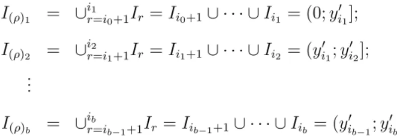
3.1 Random Time Grid 34
I(ρ)1 = ∪
i1
r=i0+1Ir =Ii0+1∪ · · · ∪Ii1 = (0;y
′
i1]; I(ρ)2 = ∪
i2
r=i1+1Ir =Ii1+1∪ · · · ∪Ii2 = (y
′
i1;y
′
i2]; ...
I(ρ)b = ∪
ib
r=ib−1+1Ir =Iib−1+1∪ · · · ∪Iib = (y
′
ib−1;y
′
ib].
Note that the elements of the set ρ are the indexes of failure times of the new intervals. Moreover, given the random partition ρ, it is assumed that:
h(t) = λr ≡λ(ρ)j, (3.14)
it means that each of the failure rates associated to the intervals that were united are equal in distribution. The scheme in the Figure 3.2 illustrates the step-by-step that is performed to estimate the time grid, aiming at providing a better understanding.
τ′ ={0, y′
1, y2′, y′3, y4′, y′5}
↓
I1 = (0, y′1]
| {z }
λ1
; I|2 = (y{z1′, y′2}]
λ2
; I|3 = (y{z2′, y′3}]
λ3
; I|4 = (y{z3′, y′4}]
λ4
; I|5 = (y{z4′, y5′}]
λ5
↓
I={0,1,2,3,4,5} →ρ={i0 = 0, i1 = 1, i2 = 3, i3 = 5}
↓
I(ρ)1 = (0, y
′
1]
| {z }
λ(ρ)1
; I(ρ)2 = (y
′
1, y3′]
| {z }
λ(ρ)2
; I(ρ)3 = (y
′
3, y5′]
| {z }
λ(ρ)3
Figure 3.2: Illustration of the intervals’ grouping scheme.
In the case of the mentioned figure there were initially five intervals: I1,I2,I3,
I4andI5, with{y1′, y′2, y3′, y′4, y5′}as endpoints. Therefore,I={0,1,2,3,4,5}and, initially,
h(t) = λj, t ∈ Ij. After that, a random partition of I was chosen: ρ = {i0, i1, i2, i3} =
{0,1,3,5}. This random partition induces the following new set of intervals:
I(ρ)1 = ∪
i1
r=i0+1Ir=∪
1
r=1Ir =I1 = (0, y′1]; (3.15)
I(ρ)2 = ∪
i2
r=i1+1Ir=∪
3
r=2Ir =I2∪I3 = (y′1, y3′];
I(ρ)3 = ∪
i3
r=i2+1Ir=∪
5
3.1 Random Time Grid 35 Thus, given the random partition, h(t) = λ(ρ)j, t ∈I(ρ)j and, in this case, λ2 and λ3 are considered to be equal in distribution as well as λ4 and λ5.
According to Barry and Hartigan (1992), the PPM is based on the following assumptions:
i) The prior distribution of ρhas the product form:
p(ρ={i0, i1, . . . , ib}) =K−1c(I(ρ)1)c(I(ρ)2). . . c(I(ρ)b), (3.16)
whereK−1 =PC c(I(ρ)1)c(I(ρ)2). . . c(I(ρ)b) is the normalizing constant and C is the set of all possible partitions of the time grid into b intervals. In turn, c(.) is the prior cohesion, which is a quantity representing the degree of similarity between the intervals that are being grouped;
ii) Conditional on the partition ρ, the model is conditionally independent and thus, have the product form:
p(λ(ρ)|ρ={i0, i1, . . . , ib}) = b
Y
j=1
p(λ(ρ)j|ρ). (3.17)
If there is no information available about the similarity among the intervals, one can simply assume that a priori the cohesion is equal to 1 for every single one of them. That is, to use the discrete U nif ormprior.
In the case of the simplest model, with no covariates and no cure fraction, and considering the prior distribution for ρ mentioned above, the posterior distribution of (ρ|φ, D) is given by:
p(ρ|φ, D) =
Z
λ(ρ)
p(λ(ρ), ρ|φ, D)dλ(ρ) ∝
Z
λ(ρ)
L(λ(ρ), φ, ρ;D)p(λ(ρ)|φ, ρ)p(φ)p(ρ)dλ(ρ)
∝
Z
λ(ρ)
L(λ(ρ), φ, ρ;D)p(λ(ρ)|φ, ρ)dλ(ρ)
∝ (γ0)
α0
Γ(α0)
Γ(α0+η1)
(γ0+ξ1)α0+η1
b
Y
j=2
(φγj−1)φαj−1
Γ(φαj−1)
Γ(φαj−1+ηj)
(φγj−1+ξj)(φαj−1+ηj)
∝ (γ0)
α0
Γ(α0)
Γ(α1)
(γ1)α1
b
Y
j=2
(φγj−1)φαj−1
Γ(φαj−1)
Γ(αj)
(γj)αj
. (3.18)
Note that the expression (3.18) can only be obtained due to the conjugacy of
3.1 Random Time Grid 36 The algorithm to estimate the time grid that will be used in this present work is the one proposed by Loschi and Cruz (2005). Following their method, consider the random variable U representing the similarity between the intervals:
Uj =
1, ifλj =λj+1;
0, ifλj 6=λj+1
(3.19)
for j = 1,2, . . . , b−1. That is, Uj = 1 if thej −th and the (j+1)-th intervals are similar
and therefore it is fair to group them; and Uj = 0 otherwise.
The idea then, is to compare the intervals, two by two, through the predictive distribution, to verify the similarity between them. If they are similar, they are united into one interval; if they are different, they remain the same (they remain being two different intervals). To generate a sample of U, consider the quantity Rj, for j = 1,2, . . . , b−1:
Rj =
p(Uj = 1|U1 =u1, . . . , Uj−1 =uj−1, Uj+1 =uj+1, . . . , Ub−1 =ub−1, D)
p(Uj = 0|U1 =u1, . . . , Uj−1 =uj−1, Uj+1 =uj+1, . . . , Ub−1 =ub−1, D)
= p(D|ρ1) p(D|ρ0)
, (3.20)
where ρ0 and ρ1 represent different partitions, according to Uj = 0 and Uj = 1,
respecti-vely. D represents the data available.
The proposed combination of the intervals will be accepted or not according to the following condition:
Uj =
1, if Rj ≥
1−u u ; 0, otherwise.
wherej = 1,2, . . . , b−1 anduis a value from theU nif orm(0,1) distribution. In the case represented by Figure 3.2, U = (U1, U2, U3, U4) = (0,1,0,1).
Once the procedure of estimating the time grid is settled, it is possible to go forward with the estimation of the remaining parameters.
It is important to highlight that the posterior distribution ofλr,r = 1,2, . . . , m′
will be the following mixture:
p(λr|D) =
X
ij−1<r≤ij
p(λ(ρ)j|D, ρ)R(I(ρ)j|D), (3.21)
3.1 Random Time Grid 37
Including Covariates into the Model
In a study where there is not only the response variable but also some ex-planatory variables, it is interesting to include this information into the model for its importance to describe the response.
Assume that there are k explanatory variables (or covariates) available. Such covariates are included into the model in a multiplicative way through the hazard function, that is, h(t) = λ(ρ)jexp{xiβ} fort∈I(ρ)j, where β is the coefficients vector and xi is the vector of covariates of thei−th individual. Note that the baseline hazard ish0(t) =λ(ρ)j, for t∈I(ρ)j.
In this case, the likelihood is given by
L(β,λ(ρ), ρ;D) =
b
Y
j=1
n
Y
i=1
(λ(ρ)jexp{xiβ})
δijexp{−λ
(ρ)jexp{xiβ}(tij−sj−1)} (3.22)
= exp
( n X
i=1
b
X
j=1
δijxiβ
) b Y
j=1
λ
Pn i=1δij
(ρ)j exp
(
−λ(ρ)j
n
X
i=1
[exp{xiβ}(tij −sj−1)]
)
.
The aim here is to estimate, β, λ(ρ),φ and ρ. It will be assumed thata priori
the vector of coefficients β does not dependent neither on λ(ρ) nor on φ or ρ. Based on
this, it is possible to calculate some important distributions, such as the joint posterior distribution, the full conditional distributions and others.
The posterior distribution of (β,λ(ρ), φ, ρ) is given by
p(β,λ(ρ), φ, ρ|D)∝L(β,λ(ρ), ρ;D)p(β)p(λ(ρ)|β, φ, ρ)p(φ)p(ρ). (3.23)
The likelihood function as well as the prior distributions of (λ(ρ)|β, φ, ρ) and of
φ were already specified. The prior distribution forρ, in turn, will be the Bayes-Laplace prior and the vector β will be considered independent a priori, with a N ormal(0, σ2
l)
3.1 Random Time Grid 38 The parameters of interest, that is,β,λ(ρ),φandρwill be estimated according
to the following expressions:
p(β|λ(ρ), φ, ρ, D) ∝ L(β,λ(ρ), ρ;D)p(β), (3.24)
p(λ(ρ)|β, φ, ρ, D) ∝ L(β,λ(ρ), ρ;D)p(λ(ρ)|β, φ, ρ), (3.25)
p(φ|β, ρ, D) ∝
Z
λ(ρ)
L(β,λ(ρ), φ, ρ;D)p(λ(ρ)|φ, ρ)p(φ)dλ(ρ), (3.26)
p(ρ|β, φ, D) ∝
Z
λ(ρ)
L(β,λ(ρ), φ, ρ;D)p(λ(ρ)|φ, ρ)p(ρ)dλ(ρ). (3.27)
The expressions associated with these distributions are presented in the Appen-dix. It is noteworthy that the conjugacy for λ(ρ)j is maintained, that is, λ(ρ)j|(β, φ, ρ, D) still follows a Gamma distribution (see Equation (A.11)). The full conditional distribu-tion of λ(ρ)j is Gamma(α0 +η1, γ0 +ξ1) for j = 1 and Gamma(φαj−1 +ηj, φγj−1 +ξj) for j = 2, . . . , b. But at this point, differently from the case with no covariates, ξj =
n
X
i=1
exp{xiβ}(tij −sj−1), for j = 1,2, . . . , b and this quantity no longer represents the
total time under test. Nevertheless, even when covariates are included into the model it is still possible to calculate the integral involving the distribution of (ρ|β, φ, D).
Incorporating the Cure Fraction
Studies in which it is plausible to assume that a proportion of subjects will never experience the event of interest, are those which cure fraction models can be applied to. A way of verifying the coherence or necessity of using such method is by verifying if there is a plateau on the Kaplan-Meier estimator, or, in other words, if the estimate becomes constant, in a value greater than zero, at a certain point of the time and remains in that way until the end of the follow-up.
3.1 Random Time Grid 39
L(β,λ(ρ),ψ, ρ;D) =
b Y j=1 n Y i=1
exp{λ(ρ)jNiexp{xiβ}(tij −sj−1)}(Niλ(ρ)jexp{xiβ})
δij
!
n
Y
i=1
θNi
i exp{−θi}
Ni!
= b Y j=1 λ Pn i=1δij
(ρ)j exp
(
−λ(ρ)j
n
X
i=1
Niexp{xiβ}(tij −sj−1)
)!
n
Y
i=1
θNi
i exp{−θi}
Ni!
N
Pb j=1δij
i exp
( b X
j=1
δijxiβ
)!
, (3.28)
where θi = exp{ziψ}.
In turn, the likelihood function based only on the observed information is:
L(β,λ(ρ),ψ, ρ;Dobs) =
X
N
L(β,λ(ρ),ψ, ρ;D)
= b Y j=1 λ Pn i=1δij
(ρ)j
! n Y
i=1
θ
Pb j=1δij
i exp
( b X
j=1
δijxiβ
) exp ( − b X j=1
δijλ(ρ)jexp{xiβ}(tij −sj−1)
)
(3.29)
exp
(
−θi 1−exp
(
−
b
X
j=1
λ(ρ)jexp{xiβ}(tij−sj−1)
)!)
.
Therefore, the parameters to be estimated are: β, λ(ρ), φ, ψ and ρ.
Mo-reover, once N is a latent variable, it is necessary to generate the number of the com-petent cells for the n individuals. It can be demonstrated (Ibrahim et al., 2001b) that (Ni|β, λ(ρ)j,ψ, Dobs)∼ P oisson(S(ti|β,λ(ρ)) exp{ziψ}) +δi, where δi is the indicator of censorship, for i= 1,2, . . . , n.
The posterior distribution of (β,λ(ρ), φ,ψ, ρ) is given by:
p(β,λ(ρ), φ,ψ, ρ|D)∝L(β,λ(ρ),ψ, ρ;D)p(β)p(λ(ρ)|β, φ, ρ)p(φ)p(ψ)p(ρ) (3.30)
The likelihood function based on all the information will be used to estimate
λ(ρ), φ, ψ and ρ. In turn, for the vector β the likelihood function based only on the
3.1 Random Time Grid 40 convergence of the parameters by eliminating the uncertainty arising from N. So, the parameters of interest will be estimated according to the following:
p(β|λ(ρ), φ,ψ, ρ, Dobs) ∝ L(β,λ(ρ),ψ, ρ;Dobs)p(β), (3.31)
p(λ(ρ)|β, φ,ψ, ρ, D) ∝ L(β,λ(ρ),ψ, ρ;D)p(λ(ρ)|β, φ, ρ), (3.32)
p(φ|β,ψ, ρ, D) ∝
Z
λ(ρ)
L(β,λ(ρ),ψ, ρ;D)p(λ(ρ)|β, φ, ρ)p(φ)dλ(ρ), (3.33)
p(ψ|β,λ(ρ), φ, ρ, D) ∝ L(β,λ(ρ),ψ, ρ;Dobs)p(ψ), (3.34)
p(ρ|β, φ,ψ, D) ∝
Z
λ(ρ)
L(β,λ(ρ),ψ, ρ;D)p(λ(ρ)|β, φ, ρ)p(ρ)dλ(ρ). (3.35)
The expressions related to these distributions can be found on the Appendix. Note once more that, even when considering a cure fraction, the conjugacy is maintained: λ(ρ)1 ∼Gamma(α0+η1, γ0+ξ1) andλ(ρ)j ∼Gamma(φαj−1+ηj, φγj−1+ξj) forj = 2, . . . , b but, at this point, ξj =
n
X
i=1
Niexp{xiβ}(tij −sj−1). Thus the the integral related to the
41
4 Applications
In order to evaluate the progress of this work, some applications were made. In total there are two applications: the first one illustrates the case of the simple model and the second one, the inclusion of the cure fraction. In both applications the estimates were obtained by using the fixed and the random time grid, so it could be possible to compare the pros and cons of each approach. It is noteworthy that regardless of the methodology applied to the time grid, the discount factor was considered unknown and thus, it was estimated.
The computational methods used in this work were the Gibbs Sampler and the Adaptive Rejection Sampler (ARS) (Gilks and Wild, 1992). The ARS method is used to generate values from a distribution when its expression does not have a closed form. To use the ARS, the functions of interest, for example, the kernel of the full conditional distributions, must be log-concave. By definition, if a function f(x) is log-concave, this means thatf′(x) decreases monotonically with increasing x, in its domain. If the function is not log-concave, the Adaptive Rejection Metropolis Sampling within Gibbs Sampling (ARMS) (Gilks et al., 1995) can be used. More information about these methods can be found in Gamerman and Lopes (2006).
All analyzes were performed by using the R software, version 3.1.2 (R Core Team, 2014). The package required to use the command “ars” was the “dlm” package (Petris, 2010). An important argument of this command is the domain of the function. It is well-known that the domain of the coefficients (β and ψ), is (−∞,∞); however, to facilitate the computational aspects related to generating values of the full conditional distributions of the coefficients, the logit transformation was applied. That is, βtrans =
exp{β}
1 + exp{β} and ψtrans =
exp{ψ}
1 + exp{ψ}, in this way, the domain of the transformation is
(0,1) and can be used in the R function.