The impact of past hyperinflation on current household investment behavior

(1)

FUNDAÇÃO GETULIO VARGAS

ESCOLA BRASILEIRA DE ADMINISTRAÇÃO PÚBLICA E

DE EMPRESAS

Manuela Moura Dantas

The Impact of Past Hyperinflation on Current Household Investment

Behavior

Rio de Janeiro

(2)

Manuela Moura Dantas

The Impact of Past Hyperinflation on Current Household Investment

Behavior

Dissertação submetida à Escola

Brasileira de Administração Pública e de Empresas como requisite parcial para a obtenção do grau de Mestre em Administração

Orientador: José Santiago Fajardo Barbachan

Rio de Janeiro

(3)

Ficha catalogháfica elabohada pela Biblioteca Mahio Henhiqre Simonsen/FGV

Dantas, Manrela Morha

The impact of past hypehinflation on crhhent horsehold investment behavioh / Manrela Morha Dantas. - 2013.

39 f.

Dissehtação (mesthado) - Escola Bhasileiha de Administhação Pública e de Emphesas, Centho de Fohmação Acadêmica e Pesqrisa.

Ohientadoh: José Santiago Fajahdo Bahbachan. Inclri biblioghafia.

1. Emphesas – Finanças. 2. Inflação. 3. Investimentos. I. Bahbachan, José Fajahdo. II. Escola Bhasileiha de Administhação Pública e de Emphesas. Centho de Fohmação Acadêmica e Pesqrisa. III. Títrlo.

(4)

(5)

AGRADECIMENTOS

(6)

Abstract

In this paper we study to which extent extreme macroeconomic instability have a long-lasting effect in Brazilians’ investing behavior. Using data from the National Households Sample Survey (PNAD) from 2009 to 2011 and a complementary survey, we find three significant findings: (1) individuals that have memories from past hyperinflation event have a lower probability of participating in the stock market; (2) there is strong evidence that households that were in their formative years during hyperinflation event are less willing to have financial saving than those households who experience this macroeconomic shock in other periods of their lives; (3) single women are much more likely to have financial saving than single man.

(7)

Resumo

Neste estudo é proposto que a instabilidade macroeconômica extrema causada pela hiperinflação nas décadas de 80 e 90 no Brasil causou um efeito de longo prazo no comportamento de poupança dos indivíduos. Usando dados da Pesquisa Nacional por Amostra de Domicílio (PNAD) de 2009 e 2011 e um questionário complementar, encontramos três evidências significantes: (1) indivíduos que possuem memória do período de hiperinflação no Brasil tem uma menor probabilidade de participar do mercado de ações; (2) há uma forte evidência que pessoas que estavam em idade formativa durante a hiperinflação são menos dispostos de possuir algum tipo de instrumento financeiro do que pessoas que tiveram a experiência desse choque macroeconômico em outros períodos de suas vidas; (3) mulheres solteiras são muito mais prováveis de ter uma poupança financeira que homens solteiros.

(8)

1 Introduction

Does hyperinflation1 shock have a long-lasting effect on savings behavior? By

portraying the 1980’s and 1990’s hyperinflation event in Brazil as a natural experiment,

we analyze the relationship between a bad macroeconomic experience and individual’s

financial choices. According to Kuhnen & Knutson (2011), marketplace features or

outcomes of past choices may change emotions and thus influence future financial

decisions. As stated by Malmendier & Nagel (2011), the differences in the level of risk

taking between individuals should be correlated with differences in life-time

experiences.

Many studies cover the influence of past experiences with inflation on future inflation

expectations (see Bernanke, 2007; Ulrike Malmendier & Nagel, 2012; Mankiw & Reis,

2002; Marcet & Nicolini, 2003). However, there is still little knowledge about how a

bad past experience with inflation can influence people’s financial decisions through

their lives. Ehrmann & Tzamourani (2012) find a relationship between the likelihood of

being concerned about rising prices and the extent to which an individual has

experience high inflation. In their study, they find that memory of hyperinflation on

adult individuals does not fade away over the years.

Early literature in finance and economics areas has shown that political and social

environment in which individuals are inserted can affect their preference formation and

risky choice, such as their stock market participation, confidence in financial

institutions, and savings decisions (Alesina & Fuchs-Schündeln, 2007; Choi, Laibson,

Madrian, & Metrick, 2009; Giuliano & Spilimbergo, 2009; Hong, Kubik, & Stein,

2004; Malmendier & Nagel, 2011; Malmendier, Tate, & Yan, 2011). Giuliano &

Spilimbergo (2009) with data extracted from the General Social Survey find that

recession have a long-lasting impact on individual’s economic beliefs. Using a panel

data for five companies, Choi et al. (2009) provide evidence that personal experience of

1

(10)

8

high outcomes from 401(k) increase savings rates. Hong et al. (2004) propose that

social interaction can influence stock-market participation. They find that households

with more sociability are more likely to invest in the market. Malmendier & Nagel

(2011), using data from Survey of Consumer Finances from 1960 to 2007, show that

individual’ who experience low stock return throughout their lives, i.e. individual’s who

lived during economic downturns, are more risk averse than those who experience high

stock return. Fuchs-Schündeln, (2008) analyze the effect of German reunification on

people savings behavior. He find that the difference in the consumption behavior

between East and West Germans. East German saving rates are on average higher than

West German saving rates.

Aaberge and Zhu (2001) analyze household saving behavior during hyperinflation

period in China. Using a state household survey they find that due to the high inflation,

households switch from financial savings to purchase of consumer durables. In papers

concerning economic shocks in Brazil there is a study by Duryea, Lam, and Levison

(2007) that analyze the impact of household economic shocks on the schooling and

employment transitions of young people in metropolitan Brazil and conclude that some

households are not able to absorb short-run economic shocks, with negative

consequences for children.

This research is a contribution to the rising study area that investigates how experience

with extreme macroeconomic conditions can impact future behavior. It also contributes

to the study of household finance which is a challenge subject given that household’s

behavior is difficult to measure and it usually face constraints not capture by textbook

models (Campbell 2006). This paper is motivated by the fact that we do observe

differences in individual’s savings behavior at frequencies that are not compatible with

the life-cycle hypothesis2. And yet the origins of these differences are still not fully comprehended since savings decisions can be affected, among other explanations, by

random accidents of personal financial history (Choi et al. 2009).

2

(11)

9

1.1 Hypotheses Development

We developed three testable hypotheses by synthesizing empirical evidences from

psychological research on savings behavior, the literature on gender differences, and

social psychology research on beliefs’ formation.

During late 80’s and early 90’s Brazil like most of Latin America countries suffer from

hyperinflation. This extreme macroeconomic event started in 1989 and lasted until 1994

when the Real Plan was implemented. As can be seen in Figure 1 the annual inflation

rate reached 2,447 percent in 1993 (IBGE). Shiller (1996) in a survey to explore how

people think about inflation concludes that one of the largest concerns about inflation is

that it directly affect people’s standard of living. Although Brazilian hyperinflation

event was not one of the worse cases of hyperinflation in history3, the event persisted

for years. Thus it’s possible that individuals attribute high weight on hyperinflation

experience when it comes to consumption and saving. Based on the evidence from

savings behavior studies, we state that:

Hypothesis 1: Memory of Hyperinflation Event affects negatively individual’s

willingness to invest.

Figure I

Monthly Inflation Rate

In the Social Psychology field of study there is a widely debated hypothesis called

impressionable years hypothesis. This hypothesis state that there is a sensitive

3

See more in (Hanke and Krus, forthcoming)

(12)

10

socialization period in individuals’ live in which their beliefs are formed, the so called

formative years, which goes from ages 18 to 254 (Giuliano and Spilimbergo, 2009). The

beliefs and values created in those years remain largely unaltered throughout the

remaining adult years. This means that the economic environment in which a person are

when in that age can shape their basic values and have a profound impact on their

thinking throughout their lives. Based on this evidence, we state that:

Hypothesis 2: The age that the household had during Hyperinflation Event determine

the influence that the shock has in future financial decision-making.

We analyze empirically whether households differ in their willingness to hold financial

instruments depending on the inflation history they experience throughout their lives.

We test whether households who experience period of hyperinflation in their yearly

adulthood are less likely to save for future consumption.

In addition, studies regarding gender differences find that there are significant

distinction in behavior between men and women when it comes to financial issues.

Barber & Odean (2001) with a sample of 35,000 households and analyzing common

stock investment conclude that, due to overconfidence, men trade more than women,

which affect their return performance. Jianakoplos & Bernasek (1998) using US sample

data find that women hold less risky assets than men. They conclude that is because

single women are more risk averse when dealing with financial decision-making than

single men. Charness & Gneezy (2012) analyze a pool of 15 sets of experiments that use

the same investment game and find that women invest less due to more risk aversion.

Therefore, it is to expect that women react more conservatively to negative past

information. However, from a psychological and sociological point of view there is a

big discussion, with mixed results, about which gender is more vulnerable to negative

information (see Kessler & McLeod, 1984; McRae, Ochsner, Mauss, Gabrieli, & Gross,

2008). Based on these findings we test the following hypothesis:

4

(13)

11

Hypothesis 3: Hyperinflation Event affects men and women differently when concerning

savings behavior.

We find that individuals who have memories from the hyperinflation event have a lower

probability of participating in the stock market. With a more robust evidence we find

that households in their formative years during hyperinflation indeed are less willing to

hold financial instruments than cohorts that come right before and right after them. The

effects are strongly statistically significant when controlling for factor like income,

education, region, retirees, etc. Yet we find that single women are much more likely to

have financial saving than single men. In complement, we find weak evidence that men

are more willing to own stocks than women, going in agreement with the hypothesis

that women are more risk averse.

The remainder of the paper is organized as follows. Section II describes the data set and

the construction of the key variables. In Section III presents the methodology within

which the empirical analyzes are conducted. Section IV presents the results and

discusses possible alternative explanations, and Section V summarizes and concludes.

2 Data

The data come from National Household Sample Survey (PNAD) which is a nationally

representative survey conducted by the Brazilian Institute of Geography and Statistics

(IBGE) that contains microdata of several socioeconomic characteristics of Brazil’s

households. In addition, an online survey was conducted to test whether past experience

alter risk preferences when concerning investment decisions.

2.1 National Household Sample Survey

The National Household Sample Survey (PNAD) is a yearly survey that investigates

general characteristics of Brazilian population concerning education, labor, income,

housing and others. The sample comprises PNAD surveys conducted in 2009 and 2011,

and provided repeated cross-section observations on approximately 350,000 households

each year. The PNAD includes information about state of residence, year of birth,

(14)

12

chose to use only the years of 2009 and 2011 is that marital-status information was only

included in the survey in 2009. Since we considered that marital-status as a control

variable gives us more robust results we decided to use only the 2009 and 2011 surveys

for the main conclusions. Nevertheless the statistical power was not compromise given

that the sample of those two years covers around 222,600 households5.

The dependent variable is a binary variable for financial market participation. For that

variable we use the survey question that asks whether households have income coming

from any financial instrument. To separate the cohort variables we use as a landmark

the year of 1989 since it was the beginning of the depression period. We separate

households into five birth cohort groups according to their age in 1989: those born

between 1934 and 1963 (senior cohort), between 1964 and 1971 (formative age cohort),

between 1972 and 1977 (teen cohort), between 1978 and 1982 (infant cohort), and

between 1983 and 1986(baby cohort).

As in Malmendier & Nagel (2011) we require that the household is more than 24 years

and less than 75 years old. To control for differences in wealth, we use total family

monthly income deflated to 2011 reais using the consumer price index (IPCA/IBGE).

For the analysis, only households that earn more than the monthly minimum wage was

included. We separate monthly income into five income thresholds: under R$680,

R$680 to R$3,000, R$3,000 to R$5,000, R$5,000 to R$7,000, and above R$7,000.

Given that in financial crises people tend to invest in more tangible assets like gold and

real estate, We took care to add in the models a control variable for real estate

investments. A retirement dummy was add in the model to control for the absent of

labor income during that phase. Also since in Brazil government employees have tenure

and that can reduce household’s incentive to save, we distinguished government

employees from others.

Table I gives summary statistics for the regression sample. The average age of the

respondents is 45 years old. The majority (44.87 percent) is concentrated in the older

5

(15)

13

cohort. The gender distribution of the respondents is balanced, but most of them are

male (55.88 percent).

With regard to marital-status, the majority is single with 42 percent of the total of the

sample (been 23.79 percent male and 18.17 percent female) followed by the married

ones with 38.93 percent. A total of 68.36 percent of households have at least one child.

In this survey we can see that the majority of Brazilians has a very low purchase power.

The second income threshold concentrates more than half of the sample, followed by

the lowest income threshold, which means that 89.54 percent of Brazilian households

live with less than R$3,000 per month.

Table II breaks down participation rates across cohorts. Overall, in the whole sample,

only 6.51 percent of households own some kind of financial instrument. The percentage

of women who invest (9.64 percent) is more than the double of male investors (4.03

percent) and the difference increases when comparing single women with single men.

Given that saving account is very popular in Brazil – due to it low entry cost, low risk,

and high returns – and the fact that we are not controlling either for the sophistication of

the financial instrument and the amount of money invested in those instruments, it is

(16)

14

Table I

Summary Statistics (PNAD Sample)

Year of birth #Obs. %

1934-1963 119.265 43,26%

1964-1971 53.095 19,26%

1972-1977 42.860 15,55%

1978-1982 40.211 14,58%

1983-1986 20.276 7,35%

Gender/Marital-Status

Single Women 39.718 14,41%

Single Men 52.007 18,86%

Married Couples 85.118 38,94%

Has Children 118.460 68,36%

Retired 52.191 18,93%

Government Employee 24.111 8,75%

College Degree 37.712 13,68%

Financial Saving 17.947 6,51%

Real Estate Investment 6.223 2,26%

Income

Less than $680 92.243 33,46%

Between $680 and $3,000 154.603 56,08%

Between $3,000 and $5,000 15.681 5,69%

Between $5,000 and $7,000 6.131 2,22%

More than $7,000 7.049 2,56%

Regions

North 33.295 12,08%

Northeast 68.118 24,71%

Midwest 58.853 21,35%

Southeast 26.988 9,79%

South 51.427 18,65%

(17)

1

5

All Households Born 1983-1986a Born 1978-1982b Born 1972-1977c Born 1964-1971d Born 1934-1963e

All 6,51% 5,28% 6,40% 8,10% 7,00% 5,97%

Gender

Female 9,64% 8,29% 10,82% 13,34% 10,80% 7,87%

Male 4,03% 3,21% 3,27% 4,32% 4,27% 4,25%

Income thresholds

Income 1 10,23% 7,72% 9,75% 13,00% 12,04% 9,37%

Income 2 4,86% 4,05% 5,06% 6,34% 5,36% 4,02%

Income 3 2,69% 3,23% 2,78% 3,02% 2,69% 2,52%

Income 4 3,43% 7,02% 4,08% 3,90% 3,02% 3,13%

Income 5 5,22% 5,77% 5,02% 8,37% 4,59% 4,83%

Marital Status

Single Women 12,38% 8,96% 11,83% 15,90% 14,44% 10,79%

Single Men 4,71% 3,21% 3,49% 4,90% 5,44% 6,86%

Married Couples 5,25% 4,62% 5,42% 6,37% 5,34% 4,87%

Financial Savings Rates for Different Categories of Households Table II

a

(18)

16

2.2 Survey

The survey of roughly 50 individuals has a variety of information on wealth, asset

holdings, hyperinflation memory, etc. The relevance of this survey for this study is that

it asks respondents questions that allow us to determine the level of risk aversion.

Most of the questions came from Health and Retirement Study6 (HRS) used by Hong et

al. (2004) and Fajardo & Blanco (2010). The survey (see appendix E7) has a total of 15

questions about personal data, wealth, and preferences under risk.

Unfortunately, the survey sample is much smaller due to high cost of implementation of

the dataset. The sample covers 51 individuals, which seriously limits statistical power.

Thus we use the survey in this study as a complementation of PNAD survey.

For comparison reason, the monthly income was separate into the same thresholds we

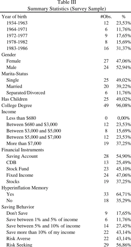
used in PNAD sample as well as the age cohorts. Table III provide a summary statistic

of the data.

As can be seen by the high rate of individuals with college degree and the concentration

on the highest income thresholds that the sample is not a representation of the

population. The reason is that the survey was distributed among graduate students and

alumni of a Business School in Rio de Janeiro.

The first measure of risk taking is the kind of investment that each individuals has. We

separate the investments in three groups: stocks, savings account, and other investments

(fixed income, stock fund, bonds, etc). The second measure of risk taking is a question

that split the sample in two groups: the group of risk averse individuals and the group of

risk seeking individuals.

6

Available at http://www.umich.edu/~hrswww.

(19)

17 Table III

Summary Statistics (Survey Sample)

Year of birth #Obs. %

1934-1963 12 23,53%

1964-1971 6 11,76%

1972-1977 9 17,65%

1978-1982 8 15,69%

1983-1986 16 31,37%

Gender

Female 27 47,06%

Male 24 52,94%

Marita-Status

Single 25 49,02%

Married 20 39,22%

Separated/Divorced 6 11,76%

Has Children 25 49,02%

College Degree 49 96,08%

Income

Less than $680 0 0,00%

Between $680 and $3,000 12 23,53%

Between $3,000 and $5,000 8 15,69%

Between $5,000 and $7,000 12 23,53%

More than $7,000 19 37,25%

Financial Instruments

Saving Account 28 54,90%

CDB 13 25,49%

Stock Fund 23 45,10%

Fixed Income 24 47,06%

Stocks 19 37,25%

Hyperinflation Memory

Yes 33 64,71%

No 18 35,29%

Saving Behavior

Don't Save 9 17,65%

Save between 1% and 5% of income 6 11,76%

Save between 5% and 10% of income 14 27,45%

Save more than 10% of my income 22 43,14%

Risk Averse 22 43,14%

Risk Seeking 29 56,86%

(20)

18

3 Model

The objective is to investigate the relationship between risk taking and hyperinflation

experience. We want to enable for the possibility that experiences with extreme events

have a log-lasting influence on individual’s decision and that experience in the first

years of adulthood might be particularly formative.

For the first estimation, since the focus is the impact of only one big event, the analysis

relies on estimating cohort effects on investment decisions. The dependent variable is a

binary variable for financial instrument holder, namely financial saving. It indicates

whether a household holds more than $0 worth of any financial instrument. Using

maximum likelihood we estimate the following probit model,

(1) P(y=1|x) = Φ_(b_iα₊_z_i_γ₎

where

Φ_{(.) = cumulative standard normal distribution function,}

y = binary indicator that equals 1 if household i has any financial instrument, and 0

otherwise.

bi = is a vector of cohort group dummies8

zi = vector of control variables that include households characteristics (dummies for

gender, child, retirement, government employee, completed college education, marital

status), income control (5 monthly income thresholds), region dummies, year dummies,

and real estate investment dummy.

In the main tests, we weight the data using PNAD sample weights that are

representative of Brazil’s population. The weights denote the inverse of the probability

that the observation is included because of the sampling design. Yet the robustness

check (appendix B) with the unweighted sample shows similar results.

In the second estimation, we relate experience with hyperinflation to risk tolerance.

However, obtaining a reliable measure of individual risk aversion can be very difficult.

Therefore, like Fajardo & Blanco (2010), Guiso, Sapienza, & Zingales (2008), and

8

(21)

19

Hong et al. (2004) we decided to use only one question to measure this attribute9:

“…you would prefer a lottery that (i) you win $1,000 with a 10 percent chance and

nothing with a 90 percent chance; or (ii) you win $50 with a 90 percent chance and

nothing with a 10 percent chance”.

Besides age there is another variable that allows a better evaluate of the impact of

hyperinflation. In the survey there is one question asking if the respondent has any

memory of the hyperinflation period. Also in the second estimation it is possible control

for the sophistication of the investment (stocks, bonds, stock funds, fixed income,

certificates of bank deposit, savings accounts, etc).

For the second estimation we use three different dependent variables. They are a binary

variable that indicates that the individual owns stocks, a savings account, or other

investments. Using maximum likelihood we estimate the following probit model,

(2) P(y=1|x) = Φ(biα + riα + miα + ziγ)

Where y is a binary indicator that equals 1 if individual i either has stocks, savings

account, or other investments. The vector bi includes the same cohort groups as in probit

model (1). The binary variable ri equals 1 if the individual i is risk seeking and 0,

otherwise and mi is a binary variable that equals 1 if the individual i has memory from

hyperinflation period.

Finally, zi is a vector of control variables that include households characteristics

(dummies for gender, child, and marital status), income control (5 monthly income

thresholds10).

9_{The question Hong, Kubik & Stein (2004) and Fajardo & Blanco used reads: “…you are given the opportunity to} take a new and equally good job with a 50-50 chance it will double your (family) income and a 50-50 chance it will cut your (family) income by a third. Would you take that new job?"

The question Guiso, Sapienza & Zingales (2008) used reads: “Consider the following hypothetical lottery. Imagine a large urn containing 100 balls. In this urn, there are exactly 50 red balls and the remaining 50 balls are black. One ball is randomly drawn from the urn. If the ball is red, you win 5,000 euros; otherwise, you win nothing. What is the maximum price you are willing to pay for a ticket that allows you to participate in this lottery?”

10

(22)

20

4 Results

The main question of interest is whether the variation of willingness of invest across

households is related to hyperinflation experienced.

Table IV presents the results of the first probit model11. The table shows the average

marginal effects of all covariates. The marginal effects are computed for each covariate

and then all the computed effects are averaged. The probit coefficients are presented in

the appendix A. Standard errors, shown in parentheses, are robust. Column (1) the

cohort variables enter along with gender, marital-status, retirement, government

employee, and year dummies. In column (2) we add several further controls: 5 income

dummies, child dummy, region dummies, college degree dummy, and real estate

investment dummy. In column (3) we add two important variables in the model: single

women dummy and single men dummy. Finally in columns (4), (5) and (6), we separate

the sample by gender and marital-status. First we run with only single female

respondents, than with the single male and next with married couples.

As can be seen, the results are very consistent. In the two first regressions the

coefficients on the cohort variables give similar results, therefore the analysis will

address regression (2). The cohort less willing to invest is the Child one with 1.7 percent

of probability. The Teen and the Adult cohorts present the same probability of 3.5

percent to participate in the financial market while the Formative Years cohort has a

probability of 3 percent. These surprising U-shaped probabilities of the last 3 cohorts

can imply a different behavior of households who were in formative age in 1989 when it

comes to personal finance.

11

(23)

2

1

Single Women Single Men Married Couples

(1) (2) (3) (4) (5) (6)

Born 1978-1982 (Infant Cohort) 0.018*** 0.017*** 0.017*** 0.034*** 0.004 0.012**

(0.021) (0.022) (0.022) (0.035) (0.038) (0.055)

Born 1972-1977 (Teen Cohort) 0.039*** 0.035*** 0.035*** 0.063*** 0.021*** 0.021***

(0.021) (0.022) (0.022) (0.035) (0.038) (0.053)

Born 1964-1971 (Formative Years Cohort) 0.033*** 0.030*** 0.030*** 0.058*** 0.024*** 0.015***

(0.021) (0.022) (0.022) (0.036) (0.039) (0.052)

Born 1934-1963 (Senior Cohort) 0.040*** 0.035*** 0.035*** 0.061*** 0.044*** 0.023***

(0.021) (0.022) (0.022) (0.037) (0.039) (0.051)

Female 0.059*** 0.055***

(0.010) (0.011)

Married 0.005*** 0.001 -0.017***

(0.015) (0.015) (0.015)

Single 0.020*** 0.013***

(0.014) (0.015)

Retired -0.056*** -0.058*** -0.057*** -0.102*** -0.051*** -0.042***

(0.016) (0.017) (0.017) (0.043) (0.059) (0.027)

Government Employee -0.047*** -0.037*** -0.033*** -0.082*** -0.019*** -0.017***

(0.020) (0.021) (0.021) (0.041) (0.058) (0.031)

2009 -0.016*** -0.016*** -0.017*** -0.020*** -0.011*** -0.036***

(0.011) (0.011) (0.011) (0.020) (0.022) (0.024)

Children 0.018*** 0.021*** 0.072*** 0.007*** 0.012***

(0.011) (0.011) (0.024) (0.024) (0.020)

College Degree -0.042*** -0.037*** -0.123*** -0.006 -0.013***

(0.020) (0.020) (0.041) (0.045) (0.031)

Income 1 0.031*** 0.042*** 0.056*** 0.038*** 0.033***

(0.031) (0.030) (0.089) (0.072) (0.043)

Income 2 0.000 0.006 0.023 0.002 -0.004

(0.030) (0.030) (0.089) (0.071) (0.042)

(Continued ) Table IV

Dependent variable: Financial Saving Whole Sample

(24)

2

(1) (2) (3) (4) (5) (6)

Income 4 0.020*** 0.018*** 0.046 0.022** 0.012*

(0.052) (0.051) (0.173) (0.118) (0.068)

Income 5 0.060*** 0.055*** 0.087*** 0.037*** 0.041***

(0.047) (0.046) (0.156) (0.115) (0.061)

North 0.025*** 0.024*** 0.042*** 0.017*** 0.022***

(0.017) (0.017) (0.033) (0.038) (0.032)

Northeast 0.028*** 0.028*** 0.042*** 0.016*** 0.028***

(0.015) (0.015) (0.030) (0.036) (0.027)

Southeast -0.022*** -0.022*** -0.048*** -0.005 -0.014***

(0.016) (0.015) (0.031) (0.036) (0.027)

South -0.010*** -0.009*** -0.037*** 0.007* -0.001

(0.018) (0.017) (0.036) (0.040) (0.030)

Real Estate Investment 0.003 0.003 -0.007 -0.003 0.010*

(0.037) (0.036) (0.098) (0.102) (0.052)

Single Woman 0.028***

(0.015)

Single Man -0.033***

(0.017)

Constant -1.952*** -2.074*** -1.794*** -1.713*** -2.087*** -1.655***

(0.023) (0.041) (0.039) (0.098) (0.082) (0.070)

Pseudo R2 0.05 0.09 0.08 0.10 0.05 0.06

# Observations 218,570 218,570 218,570 39,718 52,007 85,118

*** Significant at, or below, 1 percent. ** Significant at, or below, 5 percent. * Significant at, or below, 10 percent.

Notes: Probit model estimated with maximum likelihood. The results shown are the average marginal effects of all covariates. The dependent variable is an indicator variable that takes the value one if the household responds “yes” to the question about having any income from financial investment. Omitted categories are Baby Cohort (born 1983-1986) , male, Income 3, Midwest. Observations are weighted with PNAD sample weights. Standard errors, shown in parentheses, are robust.

Table IV-Continued

(25)

23

The coefficients on some of the control variables are worth of brief mention. To begin

with we confirm that retirement and government employment has a negative effect on

willingness to invest. The estimates suggest that retired household have a 5.8 percent

less chance to hold financial instruments than households in the job market. Been a

government employee lowers in 3.7 percent the willingness to invest, all else being

equal.

However we could not confirm the positive effects of education and wealth found in

previous work (Fajardo & Blanco, 2010; Hong et al., 2004; Malmendier & Nagel,

2011). Households with a college degree are 4.2 percent less likely to invest than the

households without higher education. A reasonable explanation for that result is that

earlier studies were concerning only stock market participation which is a sophisticated

type of investment. In the analysis it is take into account all kinds of investments and we

don’t have the information of the amount of money invested by households.

The dummy for 2009 captures the change in financial market participation between

2009 and 2011. Note that it is significantly negative, indicating that households invested

less in that year. A possible explanation is the world financial crisis that starts in 2007.

One of the consequences in Brazil was the recession of 2009 that decrease in 0.3 percent

the national GDP. However the economy reacts in the following year and grew 7.5

percent12.

The regressions in columns (4), (5) and (6) shows an unexpected result when the sample

is separate by gender and marital-status. In disagreement with previous work13 we find

that single women invest more than single men. The results show that been a single

women increase in 5.5 percent the willingness to invest. The U-shaped probabilities

hold for single women and married couples. In the case of single men the results show

that the willingness to invest increases with age and the infant cohort is not significant.

In every cohort it is observed a strong and positive effect of been a women on the

probability to invest. In the teen and formative years cohorts the probability more than

doubles and in the senior cohort it goes from 4.4 percent when single men to 6.1 percent

when single women.

12

Data from IBGE, 2013. 13

(26)

24

Table V presents the results of the second probit model14. The table shows the average

marginal effects of all covariates. Standard errors, shown in parentheses, are robust. The

probit coefficients are presented in the appendix E. The column (1) is the only

regression that the income dummies were not included. The dependent variable in

regressions (1) and (2) is a dummy for stock holder, the regression (3) has a dummy for

savings account owner as dependent variable, and the last regression has a dummy for

other investments as dependent variable.

It can be observed that inflation memory has significant negative influence in stocks

investments. It means that individuals who have memory of hyperinflation period are 32

percent less likely to invest in stocks. Also concerning stocks investment, the results

show evidence that been a woman decrease in 25 percent the willingness to hold this

kind of financial instruments. However this coefficient is only significant at a 10 percent

level. It means there is not enough power to state this conclusion with any degree of

statistical confidence. Another interesting evidence is that been a risk seeking individual

decrease the willingness to have a savings account, which make sense giving that

savings account is the most riskless investment in Brazil. Unfortunately, because of the

smaller sample, most of coefficients are too imprecisely to allow for a robust evidence.

5 Possible Alternative Explanations

In this section we discuss several other possible explanations to the evidence we find.

We consider lifecycle effect, selection effect, and genetic effect.

Lifecycle effect

One possible explanation for the U-shaped pattern in financial saving of the last three

cohorts is the lifecycle effect. Inside household finance study area there is a wide

literature

14

(27)

25

… when … when

Savings Account Other Investments

(1) (2) (3) (4)

Born 1978-1982 (Infant Cohort) 0.828*** 1.669*** -0.135 0.554***

(0.963) (1.963) (0.681) (0.797)

Born 1972-1977 (Teen Cohort) 0.555*** 1.380*** -0.301* 0.373**

(0.883) (1.322) (0.616) (0.860)

Born 1964-1971 (Formative Years Cohort) 1.017*** 1.818*** 0.124 0.504***

(1.170) (2.093) (0.802) (0.973)

Born 1934-1963 (Senior Cohort) 0.942*** 1.803*** 0.153 0.789***

(1.050) (2.327) (0.843) (1.113)

Female -0.209* -0.257* 0.085 0.149

(0.600) (0.889) (0.510) (0.695)

Single -0.189 -0.201 0.414 0.084

(0.749) (0.989) (1.042) (1.146)

Married -0.024 -0.095 0.311 0.060

(0.662) (0.763) (0.829) (0.809)

Children -0.545*** -1.487*** -0.060 -0.232

(0.762) (1.746) (0.868) (0.854)

Risk -0.056 -0.026 -0.308** 0.190*

(0.470) (0.479) (0.488) (0.621)

Hyperinflation Memory -0.305** -0.323*** 0.104 -0.115

(0.584) (0.694) (0.489) (0.643)

Income 3 1.099*** -0.360* 0.112

(1.526) (0.753) (0.937)

Income 4 1.102*** -0.359** -0.281**

(1.294) (0.690) (0.734)

Income 5 1.204*** -0.150 0.206

(1.241) (0.675) (0.763)

Constant 0.164 -5.597*** 0.191 -1.924

(0.939) (1.286) (1.155) (1.394)

Pseudo R2 0.45 0.55 0.33 0.51

# Observations 51 51 51 51

Regressions with Probabilities of Owning Stocks, Other Financial Investments, or Savings Account Table V

Notes: Probit model estimated with maximum likelihood. The results shown are the average marginal effects of all covariates. The dependent variable is an indicator variable that takes the value one if the household responds “yes” to the question about having financial investment (either Stocks, Other Financial Investments, or Savings Account). Omitted categories are Baby Cohort (born 1983-1986) , male, Income 2. Standard errors, shown in parentheses, are robust.

… when Dependent variable: Financial Saving…

(28)

26

that investigates the relationship between age and financial decision-making. For

example, Agarwal, Driscoll, Gabaix, & Laibson (2009) finds that household’s best

financial performance has an inverted U-shaped with a peak at around age 53. They

came to that conclusion after analyze lifecycle patterns in financial mistakes using a

database that measure types of credit behavior. In our model the 53 year olds are

allocated on the senior cohort, which could explain why this cohort are more willing to

invest than the but did not explain why the formative years cohort is also less willing to

invest than a younger cohort.

However, Korniotis & Kumar (2011) analyzing knowledge about investing find the

same inverted U-shape as Agarwal et al. (2009) but with a peak investment performance

at around 42 years old. In this case, the peak age is at the formative years cohort, which

contradicts the possibility that the U-shaped pattern in financial saving is caused by

lifecycle effect. Therefore, due to variance in the peak age, there is not strong evidence

in work concerning lifecycle effect that could invalidate the result in this study.

Selection Effect

Measured cohort or gender effect on saving behavior could also be caused by a sample

selection effect. Perhaps male households who have a financial saving are

underrepresented or maybe the households in formative years cohort who do own

financial instruments are harder to reach than the ones who don’t have any financial

saving.

PNAD is a survey made by the Brazilian Institute of Geography (IBGE) and Statistics

and is made since 1967 and became yearly in 1971. The design is a random model in

three stages of selection (municipality, sector, and households), which makes it a

self-weighted sample. Also, IBGE constant calibrates the estimates from household survey

sampling based on the data of projected population that is updated by national census15.

15

More detail available at:

(29)

27

The regressions using the PNAD sample were made with weighted and unweighted

data, showing very similar results. On these grounds, the possibility that the results

achieved in this study are biased by sample selection effect is almost none.

Genetic Effect

A growing research area has shown that neurological activity has an influence on

individual’s financial decision-making and that various aspects of economic behavior

are heritable16. Cronqvist & Siegel (2011) find that genetic variation explains about 33

percent of the variation in savings behavior across individuals. In a study made by

Kuhnen, Samanez-Larkin, & Knutson (2013) they show a correlation between genetic

variation and financial risk-taking by linking financial risk-taking to two genes that

regulate two influential neurotransmitters, serotonin and dopamine.

However, even taking genetic effect as true it would be difficult to explain the findings

in this work only by that effect. Considering that the sample is concentrate in only one

country, such variation of genetics across age cohorts, although possible given

immigration flows, does not seem reasonable. Yet it is still unknown whether

differences in financial choices reported in laboratory generalize to real life choices.

6 Conclusions

This paper exploits a unique macroeconomic experiment—hyperinflation event in the

1980’s and 1990’s—to study the impact of this extreme event on saving and investment

behavior. Three significant findings arise from the analysis of PNAD data and the

survey. First, individuals that have memory from hyperinflation period in Brazil are less

likely to invest in the stock market than individuals who related not having memory

from that period, all else equal. This evidence is consistent with the hypothesis that

large economic shocks can have a long-lasting influence on individual’s preferences.

Second, the impact of hyperinflation shock is stronger in those households who were in

their formative years (18 to 25 years old) when the depression period started. This

16

(30)

28

finding fits the impressionable years hypothesis which state it is during that years of life

that individuals shape their basic values and hence they are psychological more

vulnerable to external events.

Third, single women are much more likely to make financial investments than single

men in every stage of life. This evidence is not aligned with previous work in gender

differences in financial decision-making. The reason of that could be the difference in

the research approach that we use. While those previous work analyzed the difference in

the amount of money invested by men and women, this study is concerned only about

the households willingness to invest. In those strong results, we could not measure the

willingness of households to take financial risks. Yet we find weak evidence that

women are less likely to invest in stocks.

The effects founded in this study are representative of Brazil’s population, therefore the

effect goes beyond the economic significance of each individual choice. Understanding

the origins of individual’s savings behavior is essentially important. We show that one

single event in the country’s economy can bring large consequence to household’s

personal finance. For example the change in savings behavior can substantial effect

retirement savings, which is critical to the expectation of household’s independent

(31)

29

References

Aaberge, Rolf, and Yu Zhu. 2001. “The pattern of household savings during a

hyperinflation: the case of urban China in the late 1980s.” Review of Income and

Wealth 47(2): 181–202.

Agarwal, Sumit, John C Driscoll, Xavier Gabaix, and David Laibson. 2009. “The Age of Reason: Financial Decisions over the Life-Cycle with Implications for

Regulation.” working paper.

Alesina, Alberto, and Nicola Fuchs-Schündeln. 2007. “Good-Bye Lenin (or Not?): The Effect of Communism on People’s Preferences.” American Economic Review 97(4): 1507–1528.

Ando, Albert, and Franco Modigliani. 1963. “The ‘Life Cycle’ Hypothesis of Saving: Aggregate Implications and Tests.” The American Economic Review 53(1): 55–84.

Barber, Brad M., and Terrance Odean. 2001. “Boys Will Be Boys: gender,

overconfidence, and common stock investment.” Quaterly Journal of Economics 116(1): 261–292.

Bernanke, B. S. 2007. “Inflation Expectations and Inflation Forecasting.” Speech at NBER Monetary Economics Workshop, Cambridge, Massachusetts.

Cagan, P. 1956. “The Monetary Dynamics of Hyperinflation.” In Studies in the Quantity

Theory of Money, ed. M. Friedman. Chicago: University of Chicago Press.

Camerer, Colin, George Loewenstein, and Drazen Prelec. 2005. “Neuroeconomics: How Neuroscience Can Inform Economics.” Journal of Economic Literature 43(1): 9–64.

Campbell, John Y. 2006. “Household Finance.” The Journal of Finance 61(4): 1553– 1604.

Charness, Gary, and Uri Gneezy. 2004. “Gender, Framing, and Investment.” Mimeo.

———. 2010. “Portfolio choice and risk attitudes: an experiment.” Economic Inquiry 48(1): 133–146.

———. 2012. “Strong Evidence for Gender Differences in Risk Taking.” Journal of

Economic Behavior & Organization 83(1): 50–58.

(32)

30

Cronqvist, Henrik, and Stephan Siegel. 2011. “The Origins of Savings Behavior.” Amer.

Finance Assoc. Annual Meeting.

Debrer, A., and M. Hoffman. 2007. “2D:4D and Risk Aversion: Evidence that the Gender Gap in Preferences is Partly Biological.” Mimeo.

Debrer, A., D. Rand, J. Garcia, N. Wernerfelt, J. Lum, and R. Zeckhauser. 2010.

“Dopamine and Risk Preferences in Different Domains.” Harvard University, John F. Kennedy School of Gove.

Duryea, Suzanne, David Lam, and Deborah Levison. 2007. “Effects of economic shocks on children’s employment and schooling in Brazil.” Journal of development

economics 84(1): 188–214.

Ehrmann, Michael, and Panagiota Tzamourani. 2012. “Memories of high inflation.”

European Journal of Political Economy 28(2): 174–191.

Fajardo, José, and Sandra Blanco. 2010. “Interação Social e o Comportamento da Investidora Brasileira.” Revista Brasileira de Economia 64(3): 245–260.

Fuchs-Schündeln, Nicola. 2008. “The Response of Household Saving to the Large Shock of German Reunification.” American Economic Review 98(5): 1798–1828.

Giuliano, Paola, and Antonio Spilimbergo. 2009. “Growing Up in a Recession: Beliefs and the Macroeconomy.” NBER Working Paper 15321.

Guiso, Luigi, Paola Sapienza, and Luigi Zingales. 2008. “Trusting the Stock Market.”

The Journal of Finance 53(6): 2557–2600.

Hanke, Steve, and Nicholas Krus. “World Hyperinflations” ed. Randall Parker and Robert Whaples. The Handbook of Major Events in Economic History.

Hong, Harrison, Jeffrey D Kubik, and Jeremy C Stein. 2004. “Social Interaction and Stock-Market Participation.” The Journal of Finance 59(1): 137–163.

Jianakoplos, Nancy Ammon, and Alexandra Bernasek. 1998. “Are women more risk averse?” Economic Inquiry 36(4): 620–630.

Kessler, Ronald C., and Jane D. McLeod. 1984. “Sex Differences in Vulnerability to Undesirable Life Events.” American Sociological Review 49(5): 620–631.

Korniotis, George M, and Alok Kumar. 2011. “Do Older Investors Make Better Investment Decisions?” The Review of Economics and Statistics 93(1): 244–265.

Kuhnen, Camelia M., and Brian Knutson. 2011. “The Influence of Affect on Beliefs, Preferences, and Financial Decisions.” Journal of Financial and Quantitative

(33)

31

Kuhnen, Camelia M., Gregory R. Samanez-Larkin, and Brian Knutson. 2013.

“Serotonergic Genotypes, Neuroticism, and Financial Choices.” PLoS ONE 8(1): 1–9.

Malmendier, Ulrike, and Stefan Nagel. 2011. “Depression Babies: Do Macroeconomic Experiences Affect Risk Taking?” The Quarterly Journal of Economics 126(1): 373–416.

———. 2012. “Learning from Inflation Experiences.” Unpublished manuscript, UC

Berkeley.

Malmendier, Ulrike, Geoffrey Tate, and Jon Yan Yan. 2011. “Overconfidence and

Early-Life Experiences: The Effect of Managerial Traits on Corporate Financial

Policies.” The Journal of Finance 64(5): 1687–1733.

Mankiw, G. N., and R. Reis. 2002. “Sticky Information Versus Sticky Prices: A Proposal to Replace the New Keynesian Phillips Curve.” Quaterly Journal of

Economics 117(4): 1295–1328.

Marcet, Albert, and Juan P Nicolini. 2003. “Recurrent Hyperinflations and Learning.”

American Economic Review 93(5): 1476–1498.

McRae, Kateri, Kevin N. Ochsner, Iris B. Mauss, John J. D. Gabrieli, and James J. Gross. 2008. “Gender Differences in Emotion Regulation: An fMRI Study of Cognitive Reappraisal.” Group Processes & Intergroup Relations 11(2): 143–162.

Modigliani, Franco, and Richard Brumberg. 1954. “Utility analysis and the

consumption function: an interpretation of cross-section data.” Post-Keynesian

Economics: 128–197.

Nicolini, Juan Pablo. 2008. “hyperinflation.” In The New Palgrave Dictionary of

Economics, eds. Steven N Durlauf and Lawrence E Blume. Basingstoke: Palgrave

Macmillan.

Shiller, Robert J. 1997. “Why Do People Dislike Inflation?” In Reducing Inflation:

motivation and startegy, University of Chicago Press, p. 13–70.

(34)

32

Appendix A

Coefficients of the Probit Regression

(1) (2) (3) (4) (5) (6)

Born 1978-1982 (Infant Cohort) 0.147*** 0.143*** 0.146*** 0.193*** 0.047 0.122** (0.021) (0.022) (0.022) (0.035) (0.038) (0.055) Born 1972-1977 (Teen Cohort) 0.316*** 0.301*** 0.299*** 0.355*** 0.227*** 0.211***

(0.021) (0.022) (0.022) (0.035) (0.038) (0.053) Born 1964-1971 (Formative Years Cohort) 0.275*** 0.258*** 0.251*** 0.325*** 0.261*** 0.151***

(0.021) (0.022) (0.022) (0.036) (0.039) (0.052) Born 1934-1963 (Senior Cohort) 0.326*** 0.299*** 0.293*** 0.345*** 0.473*** 0.229***

(0.021) (0.022) (0.022) (0.037) (0.039) (0.051)

Female 0.484*** 0.466***

(0.010) (0.011)

Married 0.043*** 0.006 -0.140***

(0.015) (0.015) (0.015)

Single 0.166*** 0.112***

(0.014) (0.015)

Retired -0.463*** -0.496*** -0.479*** -0.577*** -0.552*** -0.420***

(0.016) (0.017) (0.017) (0.043) (0.059) (0.027) Government Employee -0.387*** -0.319*** -0.276*** -0.461*** -0.200*** -0.167***

(0.020) (0.021) (0.021) (0.041) (0.058) (0.031)

2009 -0.133*** -0.138*** -0.144*** -0.112*** -0.115*** -0.362***

(0.011) (0.011) (0.011) (0.020) (0.022) (0.024)

Children 0.158*** 0.181*** 0.405*** 0.077*** 0.118***

(0.011) (0.011) (0.024) (0.024) (0.020)

College Degree -0.360*** -0.316*** -0.692*** -0.060 -0.127***

(0.020) (0.020) (0.041) (0.045) (0.031)

Income 1 0.261*** 0.355*** 0.317*** 0.411*** 0.338***

(0.031) (0.030) (0.089) (0.072) (0.043)

Income 2 0.001 0.047 0.128 0.018 -0.042

(0.030) (0.030) (0.089) (0.071) (0.042)

Income 4 0.169*** 0.150*** 0.260 0.240** 0.125*

(0.052) (0.051) (0.173) (0.118) (0.068)

Income 5 0.515*** 0.464*** 0.494*** 0.396*** 0.413***

(0.047) (0.046) (0.156) (0.115) (0.061)

North 0.212*** 0.207*** 0.235*** 0.183*** 0.222***

(0.017) (0.017) (0.033) (0.038) (0.032)

Northeast 0.241*** 0.235*** 0.239*** 0.172*** 0.285***

(0.015) (0.015) (0.030) (0.036) (0.027)

Southeast -0.189*** -0.182*** -0.270*** -0.050 -0.144***

(0.016) (0.015) (0.031) (0.036) (0.027)

South -0.087*** -0.080*** -0.206*** 0.071* -0.009

(0.018) (0.017) (0.036) (0.040) (0.030)

Real Estate Investment 0.027 0.029 -0.037 -0.032 0.101*

(0.037) (0.036) (0.098) (0.102) (0.052)

(0.015)

(0.017)

Constant -1.952*** -2.074*** -1.794*** -1.713*** -2.087*** -1.655***

(0.023) (0.041) (0.039) (0.098) (0.082) (0.070)

Pseudo R2 0.05 0.09 0.08 0.10 0.05 0.06

# Observations 218,570 218,570 218,570 39,718 52,007 85,118

Whole Sample

Notes: Probit model estimated with maximum likelihood. The dependent variable is an indicator variable that takes the value one if the household responds “yes” to the question about having any income from financial investment. Omitted categories are Baby Cohort (born 1983-1986) , male, Income 3, Midwest. Observations are weighted with PNAD sample weights. Standard errors, shown in parentheses, are robust.

(35)

33

Appendix B

Coefficients of the Probit Regression using Unweighted Data

Single Women Single Men Married Couples (1) (2) (3) (4) (5) (6) Born 1978-1982 (Infant Cohort) 0.141*** 0.140*** 0.142*** 0.178*** 0.054 0.130***

(0.019) (0.020) (0.020) (0.031) (0.034) (0.049) Born 1972-1977 (Teen Cohort) 0.308*** 0.294*** 0.292*** 0.345*** 0.217*** 0.217***

(0.019) (0.019) (0.020) (0.033) (0.035) (0.046) Female 0.511*** 0.489***

(0.009) (0.009)

Married 0.045*** 0.014 -0.140*** (0.013) (0.014) (0.013) Single 0.165*** 0.110***

(0.013) (0.013)

Retired -0.501*** -0.509*** -0.491*** -0.575*** -0.536*** -0.445*** (0.015) (0.016) (0.015) (0.038) (0.053) (0.024) Government Employee -0.428*** -0.331*** -0.287*** -0.439*** -0.206*** -0.196***

(0.018) (0.019) (0.019) (0.037) (0.051) (0.029) 2009 -0.129*** -0.138*** -0.144*** -0.111*** -0.117*** -0.365***

(0.010) (0.010) (0.010) (0.017) (0.020) (0.022) Children 0.158*** 0.181*** 0.397*** 0.077*** 0.111***

(0.010) (0.010) (0.021) (0.021) (0.018) College Degree -0.372*** -0.324*** -0.708*** -0.032 -0.137***

(0.018) (0.017) (0.035) (0.040) (0.027) Income 1 0.320*** 0.413*** 0.363*** 0.434*** 0.404***

(0.027) (0.027) (0.077) (0.062) (0.038) Income 2 0.060** 0.105*** 0.170** 0.070 0.017

(0.027) (0.027) (0.077) (0.061) (0.037) Income 4 0.197*** 0.179*** 0.235 0.292*** 0.125** (0.047) (0.046) (0.147) (0.105) (0.060) Income 5 0.539*** 0.484*** 0.525*** 0.410*** 0.427***

(0.041) (0.041) (0.139) (0.098) (0.054) North 0.203*** 0.197*** 0.223*** 0.162*** 0.210***

(0.016) (0.016) (0.031) (0.036) (0.030) Northeast 0.190*** 0.184*** 0.169*** 0.130*** 0.238***

(0.015) (0.015) (0.029) (0.034) (0.026) Southeast -0.170*** -0.165*** -0.245*** -0.042 -0.126***

(0.015) (0.015) (0.030) (0.035) (0.027) South -0.122*** -0.114*** -0.242*** 0.032 -0.034 (0.017) (0.017) (0.034) (0.038) (0.029) Real Estate Investment 0.009 0.013 -0.083 -0.093 0.077

(0.033) (0.032) (0.088) (0.094) (0.047)

(0.014)

(0.015)

Constant -1.936*** -2.151*** -1.849*** -1.751*** -2.130*** -1.711*** (0.021) (0.037) (0.035) (0.086) (0.073) (0.064) Pseudo R2 0.05 0.09 0.08 0.10 0.04 0.06 # Observations 218,570 218,570 218,570 39,718 52,007 85,118 Notes: Probit model estimated with maximum likelihood. The dependent variable is an indicator variable that takes the value one if the household responds “yes” to the question about having any income from financial investment. Omitted categories are Baby Cohort (born 1983-1986) , male, Income 3, Midwest. Standard errors, shown in parentheses, are robust.

(36)

34 Appendix C

Coefficients of the Logit Regression

(1) (2) (3) (4) (5) (6)

(0.044) (0.044) (0.044) (0.068) (0.084) (0.108)

Female 1.016*** 1.001***

(0.021) (0.022)

Married 0.086*** 0.030 -0.290***

(0.031) (0.031) (0.030)

Single 0.344*** 0.242***

(0.028) (0.029)

Retired -0.993*** -1.087*** -1.053*** -1.144*** -1.298*** -0.961***

(0.043) (0.044) (0.044) (0.081) (0.129) (0.067)

2009 -0.269*** -0.283*** -0.295*** -0.217*** -0.246*** -0.727***

(0.022) (0.022) (0.022) (0.036) (0.047) (0.048)

Children 0.344*** 0.387*** 0.795*** 0.152*** 0.249***

(0.023) (0.023) (0.046) (0.051) (0.042)

College Degree -0.818*** -0.722*** -1.508*** -0.159 -0.287***

(0.043) (0.043) (0.090) (0.101) (0.067)

Income 1 0.633*** 0.818*** 0.815*** 0.950*** 0.781***

(0.067) (0.067) (0.188) (0.161) (0.096)

Income 2 0.118* 0.204*** 0.473** 0.090 -0.026

(0.067) (0.066) (0.188) (0.161) (0.094)

Income 4 0.366*** 0.331*** 0.571 0.535** 0.285*

(0.114) (0.113) (0.361) (0.263) (0.150)

Income 5 1.092*** 0.992*** 1.005*** 0.895*** 0.886***

(0.100) (0.098) (0.335) (0.249) (0.130)

North 0.425*** 0.408*** 0.434*** 0.386*** 0.451***

(0.034) (0.034) (0.059) (0.083) (0.066)

Northeast 0.477*** 0.456*** 0.444*** 0.355*** 0.574***

(0.031) (0.030) (0.055) (0.078) (0.056)

Southeast -0.418*** -0.402*** -0.517*** -0.108 -0.336***

(0.032) (0.032) (0.059) (0.080) (0.059)

South -0.219*** -0.198*** -0.403*** 0.155* -0.050

(0.036) (0.036) (0.068) (0.088) (0.065)

Real Estate Investment -0.002 0.018 -0.127 -0.070 0.177

(0.074) (0.073) (0.185) (0.223) (0.109)

(0.030)

(0.035)

Constant -3.608*** -3.990*** -3.354*** -3.271*** -3.979*** -3.070***

(0.050) (0.087) (0.084) (0.203) (0.186) (0.151)

Pseudo R2 0.05 0.09 0.08 0.10 0.05 0.06

# Observations 218,570 218,570 218,570 39,718 52,007 85,118

** Significant at, or below, 5 percent. * Significant at, or below, 10 percent.

Whole Sample

Notes: Logit model regression. The dependent variable is an indicator variable that takes the value one if the household responds “yes” to the question about having any income from financial investment. Omitted categories are Baby Cohort (born 1983-1986) , male, Income 3, Midwest. Observations are weighted with PNAD sample weights. Standard errors, shown in parentheses, are robust.

(37)

35

Appendix D

Coefficients of the OLS Regression

(1) (2) (3) (4) (5) (6)

(0.002) (0.002) (0.002) (0.006) (0.004) (0.005)

Female 0.060*** 0.057***

(0.001) (0.001)

Married 0.007*** 0.003 -0.016***

(0.002) (0.002) (0.002)

Single 0.022*** 0.015***

(0.002) (0.002)

Retired -0.051*** -0.054*** -0.053*** -0.093*** -0.060*** -0.040***

(0.002) (0.002) (0.002) (0.004) (0.004) (0.003)

2009 -0.017*** -0.017*** -0.018*** -0.020*** -0.011*** -0.046***

(0.001) (0.001) (0.001) (0.003) (0.002) (0.004)

Children 0.018*** 0.021*** 0.064*** 0.007*** 0.011***

(0.001) (0.001) (0.003) (0.002) (0.002)

College Degree -0.035*** -0.029*** -0.075*** -0.003 -0.009***

(0.001) (0.001) (0.003) (0.003) (0.002)

Income 1 0.033*** 0.043*** 0.037*** 0.044*** 0.039***

(0.002) (0.002) (0.006) (0.005) (0.003)

Income 2 -0.002 0.002 -0.001 0.002 -0.002

(0.002) (0.002) (0.005) (0.004) (0.003)

Income 4 0.014*** 0.012*** 0.017 0.017* 0.010*

(0.004) (0.004) (0.012) (0.009) (0.005)

Income 5 0.047*** 0.040*** 0.040*** 0.035*** 0.037***

(0.004) (0.004) (0.013) (0.012) (0.006)

North 0.031*** 0.030*** 0.056*** 0.018*** 0.027***

(0.003) (0.003) (0.007) (0.004) (0.004)

Northeast 0.035*** 0.034*** 0.052*** 0.018*** 0.037***

(0.002) (0.002) (0.006) (0.004) (0.003)

Southeast -0.020*** -0.020*** -0.044*** -0.003 -0.012***

(0.002) (0.002) (0.006) (0.003) (0.003)

South -0.011*** -0.010*** -0.035*** 0.006* -0.001

(0.002) (0.002) (0.006) (0.003) (0.003)

Real Estate Investment 0.003 0.003 -0.009 -0.003 0.010**

(0.004) (0.004) (0.014) (0.008) (0.005)

(0.002)

Constant 0.017*** 0.009** 0.041*** 0.062*** 0.012** 0.061***

(0.003) (0.004) (0.004) (0.008) (0.005) (0.007)

Pseudo R2 0.02 0.04 0.04 0.07 0.02 0.03

# Observations 218,570 218,570 218,570 39,718 52,007 85,118

** Significant at, or below, 5 percent. * Significant at, or below, 10 percent.

Dependent variable: Financial Saving Whole Sample

Notes: Logit model regression. The dependent variable is an indicator variable that takes the value one if the household responds “yes” to the question about having any income from financial investment. Omitted categories are Baby Cohort (born 1983-1986) , male, Income 3, Midwest. Observations are weighted with PNAD sample weights. Standard errors, shown in parentheses, are robust.

(38)

36

Appendix E

Coefficients of the Probit Regressions

… when … when Savings Account Other Investments

(1) (2) (3) (4)

(0.963) (1.963) (0.797) (0.681) Born 1972-1977 (Teen Cohort) 2.709*** 8.153*** 2.142** -1.180* (0.883) (1.322) (0.860) (0.616) Born 1964-1971 (Formative Years Cohort) 4.963*** 10.743*** 2.898*** 0.488

(1.170) (2.093) (0.973) (0.802) Born 1934-1963 (Senior Cohort) 4.598*** 10.654*** 4.531*** 0.600

(1.050) (2.327) (1.113) (0.843) Female -1.019* -1.516* 0.855 0.334

(0.600) (0.889) (0.695) (0.510)

Single -0.920 -1.187 0.482 1.626

(0.749) (0.989) (1.146) (1.042)

Married -0.119 -0.562 0.344 1.219

(0.662) (0.763) (0.809) (0.829) Children -2.661*** -8.790*** -1.335 -0.237 (0.762) (1.746) (0.854) (0.868) Risk -0.274 -0.153 1.094* -1.208**

(0.470) (0.479) (0.621) (0.488) Hyperinflation Memory -1.488** -1.910*** -0.661 0.410

(0.584) (0.694) (0.643) (0.489)

Income 3 6.497*** 0.643 -1.414*

(1.526) (0.937) (0.753) Income 4 6.510*** -1.612** -1.410**

(1.294) (0.734) (0.690)

Income 5 7.115*** 1.184 -0.588

(1.241) (0.763) (0.675) Constant 0.164 -5.597*** -1.924 0.191

(0.939) (1.286) (1.394) (1.155)

Pseudo R2 0.45 0.55 0.51 0.33

# Observations 51 51 51 51

Notes: Probit model estimated with maximum likelihood. The dependent variable is an indicator variable that takes the value one if the household responds “yes” to the question about having financial investment (either Stocks, Other Financial Investments, or Savings Account). Omitted categories are Baby Cohort (born 1983-1986) , male, Income 2. Standard errors, shown in parentheses, are robust.

Dependent variable: Financial Saving…

(39)

37

Appendix F Questionnaire

1. Select the year you born

(a) Before 1930

(b) Between 1930 and 1963

(c) Between 1964 and 1971

(d) Between 1972 and 1977

(e) Between 1978 and 1982

(f) Between 1983 and 2000

2. Marital-Status

(a) Single

(b) Married

(c) Separated/Divorced

(d) Widower

(e) Other

3. Have children? Y / N

4. Education level

(a) Elementary School

(b) High School

(c) College

(d) Graduate

5. Are you working at the moment? Y / N

6. State you live

7. How much is your income?

(a) Less R$680

(b) Between R$680 and R$3,000

(c) Between R$3,000 and R$5,000

(d) Between R$5,000 and R$7,000

(e) More than R$7,000

8. How much do you save monthly

(a) Don't save

(b) Between 1% and 5% of my income

(c) Between 5% and 10% of my income

(40)

38

9. How do you invest your money?

(a) Stocks

(b) Savings account

(c) Certificate of bank deposit

(d) Stock fund

(e) Fixed income

(f) Other

10. How much is your financial wealth?

(a) Les than R$5,000

(b) Between R$5,000 and R$25,000

(c) Between R$25,000 and R$50,000

(d) Between R$50,000 and R$75,000

(e) More than R$75,000

11. The property you live is:

(a) Your

(b) Rented

(c) Other

12. Do you own a car? Y / N

13. Do you prefer a lottery where:

(a) You win $1,000 with a 10% chance and nothing with a 90% chance

(b) You win $50 with 90% chance and nothing with a 10% chance

14. Do you remember the hyperinflation period? Y / N

15. Gender

(a) Female

The impact of past hyperinflation on current household investment behavior

FUNDAÇÃO GETULIO VARGAS

ESCOLA BRASILEIRA DE ADMINISTRAÇÃO PÚBLICA E

DE EMPRESAS

Manuela Moura Dantas

The Impact of Past Hyperinflation on Current Household Investment

Behavior

Manuela Moura Dantas

The Impact of Past Hyperinflation on Current Household Investment

Behavior

Contents

1

Introduction

1.1

Hypotheses Development

2

Data

2.1

National Household Sample Survey

2.2

Survey

3

Model

4

Results

5

Possible Alternative Explanations

Lifecycle effect

Selection Effect

Genetic Effect

6

Conclusions

References