SEQUENTIAL MODELLING OF BUILDING ROOFTOPS BY INTEGRATING
AIRBORNE LIDAR DATA AND OPTICAL IMAGERY: PRELIMINARY RESULTS
Gunho Sohn*, Jaewook Jung, Yoonseok Jwa and Costas Armenakis
GeoICT lab, Department of Earth and Space Science and Engineering, York University, 4700 Keele Street, Toronto, ON M3J 1P3, Canada – (gsohn, jwjung, yjwa, armenc)@yorku.ca
Commission III WGIII/4
KEY WORDS: Airborne LiDAR, Airborne Imagery, Rooftop Modelling, Model Selection, Sequential Modelling
ABSTRACT:
This paper presents a sequential rooftop modelling method to refine initial rooftop models derived from airborne LiDAR data by integrating it with linear cues retrieved from single imagery. A cue integration between two datasets is facilitated by creating new topological features connecting between the initial model and image lines, with which new model hypotheses (variances to the initial model) are produced. We adopt Minimum Description Length (MDL) principle for competing the model candidates and selecting the optimal model by considering the balanced trade-off between the model closeness and the model complexity. Our preliminary results, combined with the Vaihingen data provided by ISPRS WGIII/4 demonstrate the image-driven modelling cues can compensate the limitations posed by LiDAR data in rooftop modelling.
1. INTRODUCTION
As a virtual replica of real world, photorealistic rooftop models has been considered a critical element of urban space modelling to support various applications such as urban planning, construction, disaster management, navigation and urban space augmentation. Recently, emerging geospatial technologies like Google Earth and Mobile Augmented Reality (MAR) urgently demand advanced methods of rooftop modelling, producing more accurate, cost-effective, and large scale virtual city models. For the past two decades, much research efforts have been made in rooftop modelling. An excellent review on the recent rooftop modelling technology was reported by Haala and Kada (2010). Recently, Rottensteiner et al. (2012) presented their preliminary results of inter-comparative experiments amongst the latest state-of-the art of rooftop modelling algorithms. However, developing a “universal” intelligent machine enabling the massive generation of highly accurate rooftop models in a fully-automated manner still remains as a challenging task. The task of rooftop modelling requires not only conducting complete classification and segmentation, but also accurate geometric and topological reconstruction. Its success is easily challenged when any of distinguishable features structuring a rooftop model is missed from given imagery. This well-known “missing data problem” is caused by various factors such as the object complexity, occlusions/shadows, sensor dependency, signal-to-noise ratio and so forth. One of promising approaches to address these problems is to combine the modelling cues detected from multiple sensors, with expectations that the limitations inherited from one sensor can be compensated by the others. In this regard, combining LiDAR point clouds and optical imagery for rooftop modelling have been exploited by many researchers (Haala and Kada, 2010). This is because the characteristics of the modelling cues obtained from two data are complementary. Compared to LiDAR point clouds, the optical imagery better provides semantically rich information and geometrically accurate step and eave edges, while it shows weakness in detecting roof edges and 3D information such as planar patches
(if only single imagery is used). However, LiDAR has somewhat opposite characteristics against the optical imagery. There are two different ways to fuse LiDAR and optical imagery: parallel and sequential approach. The parallel fusion allows each modelling cues to be extracted from two datasets in parallel. Then, a rooftop model is generated through various mechanisms recovering its spatial topology (topological relations amongst lines and planes comprising key rooftop structure) using the extracted modelling cues. A common practice in the parallel fusion process is to enhance the quality of cue extraction by assigning different roles to each of two datasets. That is, line cues were extracted mainly using optical imagery, while LiDAR data was used as for validating them or assisting the generation of new lines (Chen et al., 2005; Sohn and Dowman, 2007). A similar approach can be also found in Habib et al. (2010) and Novacheva (2008). The topological relations amongst modelling cues extracted were reconstructed in an integrated manner, for instance by partitioning LiDAR space with extracted lines using a split-merge algorithm (Chen et al., 2005) or Binary Space Partitioning (Sohn and Dowman, 2007). In contrast, the sequential fusion approach is to generate a rooftop model relying on single information source, which is later refined by the other data. For instance, Rottensteiner et al. (2002) produced rough rooftop models using LiDAR data and improved the initial model’s accuracy by fitting parametric model instances to the back-projected image of LiDAR-driven models. The sequential modelling fusion has not been studied much compared to the parallel fusion. However, we believe that the sequential fusion method will provide important roles to spatio-temporally update large-scale virtual city models where existing models can be effectively used as priors for improving its accuracy with newly acquired data. In this study, we propose a sequential rooftop modelling process, in which an initial model is improved by a hypothesis-test scheme based on Minimum Description Length (MDL). In this framework, we discuss separate roles of initial models (LiDAR-driven) and newly acquired lines (optical imagery-driven) with respect to a generative way of producing a model hypothesis space. In the next section, an overall workflow of proposed modelling
process is explained. In Section 3, our sequential fusion methods are described, followed by presenting experimental results and drawing our conclusions in Section 4 and 5.
2. OVERALL METHODOLOGY
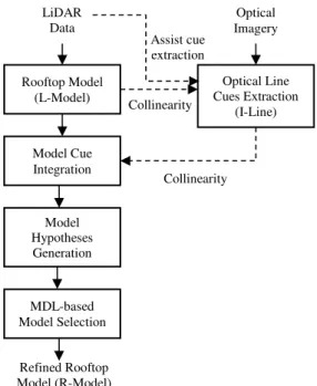
We propose a sequential modelling algorithm to improve an existing model derived from LiDAR data (L-Model) by integrating it with lines detected from single optical imagery (I-Lines). Figure 1 shows an overall workflow of proposed rooftop modelling system. An initial rooftop model is required as an input vector to the sequential modelling chain. A key of the proposed method is to create new topological features connecting between L-Model and I-Lines in an integrated manner. Newly generated lines are only allowed to change their orientations or being eliminated for producing model hypotheses. Global geometric properties (line orientation, symmetry and parallelism) of the integrated cues implicitly set the rules to generate model hypotheses. An optimal model hypothesis is determined through selective construction of model hypotheses using integrated modelling cues. The model selection criterion is designed using MDL principle, favouring more regular and simpler rooftop models as final output.
Figure 1. The overall workflow of proposed sequential modelling algorithm.
3. SEQUENTIAL ROOFTOP MODELLING
3.1 Generation of LiDAR-driven rooftop model
Our sequential modelling system requires existing rooftop models derived from Digital Surface Model (DSM) as input vectors to be improved. In current study, these initial rooftop models were generated using LiDAR point clouds by combining previous research works (Sohn et al., 2008; Sohn et al., 2012). The model processing pipeline comprises four steps: 1) classification/segmentation; 2) modelling cue extraction; 3) topology reconstruction; and 4) vector regularization. After classifying LiDAR point clouds, individual building regions were detected, from each of which a set of planes were segmented using RANSAC algorithm. Then, two different types of line primitives, intersection and step line, were extracted over plane segments. A spatial topology amongst extracted cues
(planes and lines) was constructed using Binary Space Partitioning (BSP) tree, which progressively partitions a building region into binary convex polygons (Sohn et al., 2008). BSP tree might cause topological errors, mainly due to errors introduced in line extraction. To resolve this problem, a regularization algorithm using MDL principles was adopted (Sohn et al., 2012). Given a local configuration sampled in BSP-based rooftop model, hypothetical models were produced, of which the most optimal (regularized and simplified) model was iteratively chosen using MDL criteria. Thus, the initial rooftop models from LiDAR data (L-Model) were generated. 3.2 Extraction of optical line cues
To improve existing rooftop models (L-Model), new line segments were detected from airborne imagery using Kovesi’s algorithm that relies on the calculation of phase congruency to localize and link edgels (Kovesi, 2011). Given exterior orientation information of optical sensor used, the well-known collinearity between image and object space was established. I-Line is defined as a straight line corresponding to key rooftop structures. To detect I-Lines, L-Model and its associated laser points with attributes including labels (building, non-building) and plane segmentation ids were back-projected to the imagery. I-Lines were identified if a line extracted from the imagery is found within a searching space (minimum bounding box) generated from L-model edges. I-Lines’ coordinates in 3D object space were obtained by intersection 2D I-Lines with their corresponding planes in object space using the collinearity equation. In this study, a heuristic bounding condition for the line-plane intersection between the image and the object space was assumed.
3.3 Model cue integration
The integration of I-Lines and L-Model is conducted in object space, which leads to generating new integrated modelling cues. Suppose that I-Lines and L-Model are denoted as a set of image lines, { } and model lines, { }. The first step of the cue integration is to identify a membership of to by investigating spatial relations such as proximity and intersection properties between two line sets. Note that one I-Line can belong to multiple model lines if it spans multiple model lines (1-N relation). Once the line memberships were identified, actual topological relations between two line sets were established by introducing new topological lines, { } connecting and . As shown in Figure 2, a topological relation between and needs to be established. For this purpose, ’s two guide lines, and , are generated as infinite lines of and ( ’s neighbouring lines). Then, { } are generated by generating line segments in two ways connecting with the shortest distance; 1) between and (starting and ending vertices) and 2) between and ( and ).
Rooftop Model (L-Model)
LiDAR Data
Optical Imagery
Optical Line Cues Extraction
(I-Line)
Model Hypotheses Generation Model Cue Integration
MDL-based Model Selection
Refined Rooftop Model (R-Model)
Collinearity Collinearity
Assist cue extraction
Figure 2. Establishment of topological relations between I-Line and L-Model For hypothesis generation.
3.4 Model hypothesis generation
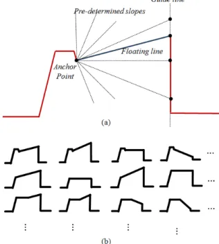
In the previous section, multiple topological relations integrating image lines with existing model lines were established. The model hypothesis generation is a process to generate possible models reflecting the contribution of image lines to the improvement of existing model (L-Model). Except , and were newly created, which needs to be not only validated, but also regularized as part of the refined rooftop model. To facilitate this task, we adopted a similar regularization method introduced by Sohn et al. (2012). In this scheme, we considered and as a floating line, which slope is changeable with pre-determined slopes (clustered in line slope spaces extracted from I-Lines and L-Model). Note that only one terminal line node (not intersected with any model line) is used as an anchor point to rotate the slope of floating line. While, ’s slope is not changeable, but used as a guide line, with which floating lines are intersected. In this way, a hypothesis model (H-Model) is generated (see figure 3).
Figure 3. Illustration of model hypothesis generation from a line
in figure 2: (a) example of hypothesis generation for floating line and (b) examples of hypotheses generated from (a).
3.5 Optimal model selection
In a discriminative modelling approach, specific model to be fit with given observation is usually not known a priori. Instead, a
decision process, called model selection, is adopted for selecting the optimal model through stochastically competing model candidates. Rissanen (1978) introduced MDL (Minimum Description Length) for inductive inference that provides a generic solution to the model selection problem (Grünwald, 2005). MDL provides a flexibility to encode a bias term, which allows us to protect against over-fitting of model of interest to limited observations. This bias is estimated by measuring the “model complexity”, which degree varies depending on the regularity (similar or repetitive patterns) hidden in observations. Weidner et al. (1995) posed building outline delineation as the model selection problem using MDL. Sohn et al. (2012) have extended it to rooftop models comprising multiple planes by implicitly generating model hypotheses. In this study, we adopted Sohn et al. (2012)’s MDL framework, which objective function is described below:
| (1)
Where, H and D indicate a building model hypothesis and its boundary associated laser points, respectively. and are weight values for balancing the model closeness and the model complexity. In Eq. (1), the closeness term represents bits encoding the goodness-of-fit between the hypothesis and its associated laser points, while the complexity term represents bits evaluating the hypothesized model’s complexity. The model selection process was conducted in the object space. 3.5.1 Closeness term ( | ): Assuming that error model between data and hypothesis follows Gaussian distribution, the closeness term in Eq. (1) can be rewritten as:
| (2)
Where Ω is the sum of the squared residuals between a model (H) and a set of observations (D), that is [ ] [ ]. Instead of using Euclidean distance, we measured Ω using a geodetic-like distance in order to favour a model hypothesis that maximizes the planar homogeneity. We first divided laser boundary points into two groups: (1) boundary points belonging to the target plane (target points), and (2) belonging to the non-target planes (non-non-target points). Ω is measure as a shortest length between a point and its corresponding model line using Euclidean distance within homogeneous region (i.e., the target point’s distance measured within the target plane or the non-target point’s distance measured within the non-target plane). In other cases, Ω is measured differently by adding a penalized distance (a minimum distance between the point and terminal nodes of its corresponding model line) to the point’s Euclidean distance to the model.
3.5.2 Complexity term ( ): The complexity term in Eq. (1) is designed to estimate the degree of geometric regularity of the hypothesized model. We consider that the geometric regularity varies depending on 1) directional patterns (the number of different direction), 2) polyline simplicity (the number of vertices), and 3) orthogonality and presence of acute angles. Three geometric regularization factors are incorporated into the complexity term as:
′ ′ ∠
∠ ′
∠ (3)
Where the subscript v, d, and ∠ indicate vertex, line direction, and inner angle; ∠ indicate the number of vertices, the number of identical line directions, and penalty value to inner angle. ( ∠ are estimated from the initial model determined at previous iteration; ( ′ ′ ∠′ are computed from model hypotheses that are locally generated as described in Section 3.2; ( ∠ are weight values for each factor. Note that grouping the inner angle and thus estimating
∠ and
∠ ′
was conducted using heuristically determined threshold.
3.5.3 Global Optimization: Let denote a set of all possible hypotheses. The optimal model is selected through the direct comparison of DLs for all model candidates in H, which has minimum DL.
(4)
3.6 Parameter estimation
In Eq. (1), the two terms, the model closeness and the model complexity, have an opposed role to one another in selecting the optimal model. If the former dominates over the latter, an over-fitted model to laser boundary points is preferred to be selected, which leads to noisy rooftop models. For the opposite case, the selected rooftop model becomes over-simplified and thus shows its high deviation from laser boundary points. In either case, unfavourable models are generated in the regularization sense. To achieve an optimal balance between two terms, we adopted the Min-Max criterion which minimizes possible loss, while maximizes gain (Gennert and Yuille, 1988). In our study, the Min-Max principle is closely related to minimizing the cost value DL and maximizing the contribution from both of two terms, thereby finding the optimal [ ] in Eq. (1). For each term, this leads to avoid the best scenario that one of two terms dominates by having excessively low or high of . To achieve this goal, the “Max” operator derives an optimal weight value by selecting the worst scenario showing the maximum DL in Eq. (1). This can be calculated by taking the first-derivative of Eq. (1) with respect to
, satisfying following condition:
| | (5)
Where H in Eq. (5) was determined at specific using Eq. (4). Considering the boundary conditions in Eq. (5), where at
and | at corresponds to zero, we can
compute biases in two terms. Thus, | and in Eq. (5) were normalized respectively with the bias quantities estimated. The “Min” operator is now applied for the selection of optimal hypothesis, H*, using Eq. (4). The above-mentioned Min-Max function is described as:
[ | | ](6)
4. EXPERIMENTAL RESULTS
We evaluated the performance of the proposed method using “Vaihingen” dataset provided by the ISPRS WGIII/4 (Rottensteiner et al., 2012). The “Vaihingen” data was acquired by Leica ALS50 system with an average point density of 6.7 points/m2 (i.e., ~0.4 m point spacing) at a mean flying height of
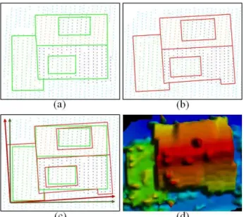
500 m above ground level. The 3D positional accuracy shows approximately 10 cm. A high-resolution pan-sharpened colour imagery was also captured from the Intergraph Z/I imaging’s DMC (Digital Mapping Camera) with the ground sampling distance of 8 cm and the radiometric resolution of 8 bits. The interior and exterior parameters were estimated in the level of 1 pixel georeferencing accuracy. Figure 4 shows an example how the proposed fusion approach can provide benefits against L-Model. Due to its irregular point acquisition, LiDAR data shows some difficulties of modelling detailed rooftop shape, resulting in the shape distortion including over-simplification and area shrinkage (Figure 4(b)). However, as can be shown in Figure 4(c), integrating image lines with L-Model demonstrates its contributions to the model improvements from Figure 4(b); enlarging the overall area and recovering the missed roof structures. Figure 5 shows another example, in which the orientation of a rooftop in L-Model is biased to LiDAR’s scanning direction. Figure 5(c) presents this problem can be resolved by adding I-Lines (lines from optical imagery), which are less affected by sensor’s specification used in data acquisition.
Figure 4. Sequential rooftop modelling process from: (a) airborne image (left) and LiDAR data (right); (b) L-Model (initial LiDAR-driven model); and (c) improved rooftop model.
Figure 5. Comparison of rooftop modelling results in building orientation;(a) L-Model, (b) sequential modelling results, (c) overlaid rooftop models, and (d) LiDAR data.
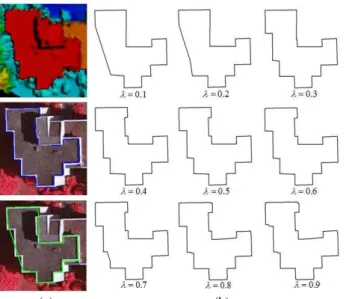
Figure 6 illustrates the effects of selecting optimal ; depending its value, different level-of-details (LoD) can be represented in rooftop models produced. As closes to 1, the
degree of model complexity, showing the tendency of over-fitted to laser boundary observations, increases, while decreasing tends to produce much simpler (over-simplified) rooftop models. It is not a trivial task to explicitly determine as it is also application specific; for example, detail models are required for decision-making on construction (Scherer and Schapke 2011), but coarse models for an urban planning (Yu et al. 2010). However, in general, we concern determining , which preserves all the detailed key structures in rooftop models, but makes the models being less sensitive to the missing data. In figure 6, was evaluated its modelling performance over discrete space as explained in Eq. (5),
. Figure 7 presents a relation between
DL values and its corresponding before and after normalizing two regularization terms in Eq. (2). As a result, with the maximum DL was changed from 0.7 (before) to 0.4 (after). Relying on our visual inspection, better model quality preserving its details and corresponding to real roof edges is shown at of 0.4, rather than 0.7. It suggests a promising effect of normalization. A sensitivity analysis of the modelling between L-Model and sequential modelling results has not been conducted yet in this study. However, figure 6 indicates that the proposed method is able to recover most of the details close to exact solution (rooftop vector at =0.4 in figure 6(b)), even over-simplified L-Model was used as an initial model (green rooftop vector in figure 6 (a)).
(a) (b)
Figure 6. Development of rooftop polygon model with respect to .
D
e
sc
r
ipti
on Le
n
gth
(
D
L*) [
bi
ts
]
Weight Value ( )
(a)
Weight Value ( )
D
e
sc
r
ip
ti
on
Le
ngth
(
D
L*) [
bi
ts
]
(b)
Figure 7. Optimal weight value ( ) before (a) and after (b) the normalization of two regularization terms.
As our preliminary experiments using “Veihingen” data, total seven buildings were selected for evaluating the overall of the proposed algorithm. In figure 8, the green and red colours denote L-Models and sequential modelling results, respectively. Our visual investigation suggests that the sequential modelling demonstrated its ability of recovering some important, but detailed roof structure and also improved the models’ edge correspondences by enlarging its area and rectifying the rooftops’ orientations. A quantitative analysis of the algorithm’s performance has been conducted with respect to area, perimeter and numbers of vertices between L-Models and its rectified models. Figure 9 shows that sequential modelling increased the rates of the three performance factors, which were confirmed as better modelling results.
Figure 8. Building models from LiDAR (green) and building models refined by image (red).
Figure 9. (a) Sum of area, perimeter, and the number of vertex of 7 test building models, respectively, (b) rate of increase of 7 test building models.
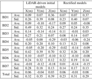
We also conducted a comparative measurement of vertices’ displacement between sequential modelling results and reference models. The reference models have been produced using the photogrammetric plotting. As shown in Table 1, the average differences in (X, Y, Z) between L-Models and reference models were reported as (0.06m, -0.04m, 0.03m) with the r.m.s.e. of (0.32m, 0.35m, 0.39m). While, the comparison of rectified models to the reference shows compatible differences of (0.06m, -0.01m, 0.08m) with lower r.m.s.e. of (0.23m, 0.31m, 0.29m), respectively in (X,Y,Z). This indicates the sequential modelling shows a positive aspect of improving the modelling accuracy. A final rooftop models over test building samples is visualized in Figure 10.
Table 1. Estimated accuracy of building models
LiDAR-driven initial models
Rectified models X(m) Y(m) Z(m) X(m) Y(m) Z(m) BD1 Ave. 0.09 0.07 0.36 0.07 0.07 0.37
Std. 0.26 0.39 0.08 0.23 0.40 0.07 BD2 Ave. 0.09 -0.10 -0.17 0.09 0.05 -0.08
Std. 0.49 0.32 0.24 0.27 0.24 0.35 BD3 Ave. 0.14 -0.14 -0.14 0.11 -0.01 0.03 Std. 0.27 0.21 0.07 0.08 0.14 0.07 BD4 Ave. -0.05 0.00 -0.29 -0.03 -0.06 -0.24
Std. 0.20 0.20 0.10 0.13 0.21 0.08 BD5 Ave. -0.05 -0.20 -0.29 -0.02 -0.14 -0.09
Std. 0.42 0.39 0.70 0.32 0.26 0.20 BD6 Ave. 0.10 -0.07 -0.10 0.12 -0.10 -0.08
Std. 0.24 0.32 0.12 0.22 0.19 0.14 BD7 Ave. -0.01 -0.12 -0.18 0.01 -0.14 -0.15
Std. 0.28 0.18 0.13 0.14 0.17 0.13 Total Ave. 0.06 -0.04 0.03 0.06 -0.01 0.08 Std. 0.32 0.35 0.39 0.23 0.31 0.29
Figure 10. 3D visualization of rooftop models produced by sequential modelling algorithm.
5. CONCLUSIONS
In this paper, we proposed a sequential modelling method to improve existing rooftop models driven from LiDAR data by incorporating lines extracted from optical imagery with the model. We suggested an implicit generation of local model hypotheses by combining lidar-driven models and image-driven lines. MDL was adopted to select optimal model by comparing competitive model candidates. A normalization of the Min-Max optimization process was introduced to improve the optimal trade-off between the model closeness and the model complexity in MDL. In this preliminary study, we confirmed
that introducing image-driven lines is able to improve rooftop modelling quality, by compensating for the inherent limitations of LiDAR data, which leads to enhancing edge correspondence, improving level-of-details and rectifying biased model orientation. In our future works, we will focus on the improvement of controlling the level-of-detail in the modelling optimization, quantitative investigation of sensitivity of initial model’s quality and incorporating the probabilistic bounds in the modelling cue integration with more extensive datasets.
ACKNOWLEDGEMENTS
This research was funded by Discovery Grant from the Natural Sciences and Engineering Research Council of Canada. We thank ISPRS WGIII/IV committee and German Society for Photogrammetry, Remote Sensing and Geoinformation (DGPF) for their assistance in preparing the Vaihingen data.
REFERENCE
Chen, L., Teo, T., Rau, J., Liu, J., Hsu, W., 2005. Building reconstruction from LiDAR data and aerial imagery. In: Proceedings of the IEEE International Geoscience and Remote Sensing Symposium, vol. 4. pp. 2846–2849.
Gennert, M. A., Yuille, A. Y., 1988. Determining the optimal weights in multiple objective function optimization. In Proc. Second Int. Conf. Computer Vision, pp. 87–89.
Grünwald, P., 2005. A tutorial introduction to the minimum description length principle. In P. Grünwald, I. J. Myung, and M. Pitt, editors, Advances in Minimum Description Length: Theory and Applications, pages 3–81. MIT Press.
Haala, N., and Kada, M., 2010. An update on automatic 3D building reconstruction. ISPRS Journal of Photogrammetry and Remote Sensing 65, 570-580.
Habib, A.F., Zhai, R., Kim, C., 2010. Generation of complex polyhedral building models by integrating stereo-aerial imagery and LiDAR data. Photogrammetric Engineering & Remote Sensing 76(5), 609-623.
Kovesi, P.D., 2011. MATLAB and Octave functions for computer vision and image processing. Centre for Exploration Targeting, School of Earth and Environment, The University of Western Australia.
Novacheva, A., 2008. Buildingroof reconstruction from LiDAR data and aerial images through plane extraction and colour edge detection. The International Archives of the Photogrammetry, Remote Sensing and Spatial Information Sciences 37(Part B6b), 53-57.
Rissanen, J., 1978. Modeling by the shortest data description.
Automatica 14, 465-471.
Rottensteiner, F., and Jansa, J., Automatic Extraction of Building from LIDAR Data and Aerial Images, IAPRS, Vol.34, Part 4, pp. 295-301, 2002.
Rottensteiner, F., Sohn, G., Jung, J., Gerke, M., Baillard, C., Benitex, S. and Breitkopf, U., 2012. The ISPRS benchmark on urban object classification and 3D building reconstruction.
ISPRS Annals, 1(3), 293-298.
Scherer, R.J., Schapke, S.E., 2011. A distributed multi-model-based management information system for simulation and decision-making on construction projects. Advanced Engineering Information, 25(4), pp. 582-599.
Sohn, G., and Dowman, I., 2007. Data fusion of high-resolution satellite imagery and lidar data for automatic building exraction.
ISPRS Journal of Photogrametry and Remote Sensing, 62(1), 43-63.
Sohn, G., Huang, X., Tao, V., 2008. Using a binary space partitioning tree for reconstructing polyhedral building models
from airborne LiDAR data. Photogrammetric Engineering & Remote Sensing 74(11), 1425-1438.
Sohn, G., Jwa, Y., Jung, J., Kim, H. B., 2012. An implicit regularization for 3D building rooftop modeling using airborne data, ISPRS Annals of the Photogrammetry, Remote Sensing and Spatial Information Sciences, Volume I-3, 2012 XXII ISPRS Congress, 25 August – 01 September 2012, Melbourne, Australia.
Weidner, U., Förstner, W., 1995. Towards Automatic Building Extraction from High Resolution Digital Elevation Models.
ISPRS Journal, 50(4), pp. 38-49.
Yu, B., Liu, H., Wu, J., Hu, Y., Zhang, L., 2010. Automated derivation of urban building density information using airborne LiDAR data and object-based method. Landscape and Urban Planning, 98(3-4), pp. 210-219.