A method for parameterising roughness and topographic sub-grid scale effects in hydraulic modelling from LiDAR data

(1)

HESSD

7, 2261–2299, 2010

A method for parameterising

A. Casas et al.

Title Page

Abstract Introduction

Conclusions References

Tables Figures

◭ ◮

Back Close

Full Screen / Esc

Printer-friendly Version

Interactive Discussion

Hydrol. Earth Syst. Sci. Discuss., 7, 2261–2299, 2010 www.hydrol-earth-syst-sci-discuss.net/7/2261/2010/ © Author(s) 2010. This work is distributed under the Creative Commons Attribution 3.0 License.

Hydrology and Earth System Sciences Discussions

This discussion paper is/has been under review for the journal Hydrology and Earth System Sciences (HESS). Please refer to the corresponding final paper in HESS if available.

A method for parameterising roughness

and topographic sub-grid scale e

_ff

ects in

hydraulic modelling from LiDAR data

A. Casas1,4, S. N. Lane2, D. Yu3, and G. Benito1

1

Institute of Natural Resources, Consejo Superior de Investigaciones Cient´ıficas, 28006 Madrid, Spain

2

Institute Hazard, Risk and Resilience and Department of Geography, Durham University, Durham, DH1 3LE, UK

3

Department of Geography, Loughborough University, Loughborough, LE11 3TU, UK

4

Department of Land, Air, and Water Resources, University of California, Davis, CA 95616, USA

Received: 16 March 2010 – Accepted: 16 March 2010 – Published: 12 April 2010 Correspondence to: A. Casas ([email protected])

(2)

HESSD

7, 2261–2299, 2010

A. Casas et al.

Title Page

Tables Figures

◭ ◮

Back Close

Full Screen / Esc

Abstract

High resolution airborne laser data provide new ways to explore the role of topo-graphic complexity in hydraulic modelling parameterisation, taking into account the scale-dependency between roughness and topography. In this paper, a complex to-pography from LiDAR is processed using a spatially and temporally distributed method

5

at a fine resolution. The surface topographic parameterisation considers the sub-grid LiDAR data points above and below a reference DEM, hereafter named as topographic content. A method for roughness parameterisation is developed based on the to-pographic content included in the toto-pographic DEM. Five subscale parameterisation schemes are generated (topographic contents at 0, _±5, _±10, _±25 and _±50 cm) and

10

roughness values are calculated using an equation based on the mixing layer theory (Katul et al., 2002), resulting in a co-varied relationship between roughness height and topographic content. Variations in simulated flow across spatial subscales show that the sub grid-scale behaviour of the 2-D model is not well-reflected in the topographic content of the DEM and that subscale parameterisation must be modelled through

15

a spatially distributed roughness parameterisation. Variations in flow predictions are related to variations in the roughness parameter. Flow depth-derived results do not change systematically with variation in roughness height or topographic content but they respond to their interaction. Finally, subscale parameterisation modifies primar-ily the spatial structure (level of organisation) of simulated 2-D flow linearly with the

20

additional complexity of subscale parameterisation.

1 Introduction

Roughness elements on a floodplain comprise both ground surface irregularities (i.e. topographic variability) and vegetation elements (trees, bushes, logs, stumps, etc.). A spatially distributed approach to any hydraulic modelling scheme must therefore be

25

(3)

HESSD

7, 2261–2299, 2010

A. Casas et al.

Title Page

Tables Figures

◭ ◮

Back Close

Full Screen / Esc

Theoretically, the topographic representation must characterise the terrain surface over which the fluid flows at an adequately discretised scale in order to reflect the flow processes of interest. Similarly, roughness parameterisation must account for energy losses due to geometric variability of the surface produced at scales finer than those represented in the mesh (discretisation scale). Clearly, both concepts are physically

5

linked by a scale-dependency, which may strongly influence two-dimensional hydraulic modelling results (Lane, 2005). A higher resolution model will explicitly encompass smaller topographic variations, provided the associated topographic data are at the same resolution. With a coarser model resolution, smaller topographic variations will need to be parameterised, either explicitly through a porosity type treatment (e.g. Yu

10

and Lane, 2006b) or upscaling of a roughness parameter. The main problem of assess-ing spatial subscale effects upon flow is that, in practice, roughness parameterisation must account not only for discrepancies between the intrinsic scale of the surface vari-ability and the scale represented in a mesh, but also for the discrepancies between the intrinsic scale of the flow process and the processes explicitly represented in the

15

numerical solution (i.e. the processes not explicitly represented because of the aver-aging of the flow equations in time or space, such as diffusive effects in the flow due to turbulence in a 2-D approach). Therefore, the roughness parameter turns out to be an effective parameter commonly obtained through a calibration procedure (e.g. Lane and Ferguson, 2005). This situation complicates the scale-dependent relationship between

20

roughness and topography.

However, the growth of hydraulic modelling applications has emphasized the im-portance and necessity of innovation in terms of processes representation, mainly in relation to boundary roughness parameterisation (Lane et al., 2004; Nicholas, 2005; Horritt, 2005) and topographic parameterisation methodologies (Casas et al., 2010;

25

(4)

HESSD

7, 2261–2299, 2010

A. Casas et al.

Title Page

Tables Figures

◭ ◮

Back Close

Full Screen / Esc

Bates, 2000; Bates et al., 2003; Suarez et al., 2005; Andersen et al., 2006; Mandl-burger and Briese, 2007; Liu 2008; Cook and Merwade, 2009) and extracting vege-tation density and height (Popescu and Zhao, 2008; Antonarakis et al., 2007, 2008) are promoting the development of new resistance formulations to link this highly de-tailed information with the spatially-averaged flow dynamics simulated by the model

5

(Katul et al., 2002; Poggi et al., 2008, 2009). LiDAR measurement principles are well established (Ackermann, 1999; Wehr and Lohr, 1999) but the processing of raw data and the accuracy of resultant modelled data are not so evident (Gomes-Pereira and Wicherson 1999; Hodgson and Bresnahan, 2004) although Marks and Bates (2000), Bates et al. (2003) and Mason et al. (2003) are important exceptions in relation to flood

10

inundation modelling. Previous research on LiDAR applications to river hydraulics has addressed not only the influence of mesh resolution of processed laser data but that of the characteristic elements that modify the measurement scale, including the raw point density scheme and flying height in the measurement scale (Hirata, 2004), but also its particular impact upon flood modelling (Raber et al., 2003; Omer et al. 2003; Gueudet,

15

2004; Haile, 2005).

One of the main di_fficulties in the use of LiDAR data is the uncertainty introduced in the DEM, namely the measurement errors due to the difficulty of separating bare earth from the rest of measured data. Low vegetation is particularly difficult to differentiate from ground measurement (Asselman 2002; Straatsma and Middelkoop, 2006).

Filter-20

ing procedures are commonly used to classify bare earth from the rest of the points. Different filtering and classification procedures or criteria will lead to different modelled ground surfaces for a certain mesh resolution. Points classified as terrain will determine the topographic content of the ground model which in combination with mesh resolu-tion determines the spatial scale of the elevaresolu-tion model. Thus, high resoluresolu-tion laser

25

(5)

HESSD

7, 2261–2299, 2010

A. Casas et al.

Title Page

Tables Figures

◭ ◮

Back Close

Full Screen / Esc

resolution. In this way, the assessment of spatial scale effects in hydraulic models can be performed by modifying exclusively the topographic content of the DEM (Casas et al., 2010).

This paper explores the role of topographic complexity considering a spatially and temporally distributed subscale parameterisation, where the roughness

parameterisa-5

tion scheme varies with the amount of high resolution geometric detail included in the topographic DEM. The main objectives are (1) to develop a subscale spatial parameter-isation methodology using LiDAR data that responds to the dependency of the model upon the topographic scale for a 2-D floodplain inundation model and (2) to assess its parameterisations’ impacts upon the magnitude and the structure of depth derived

10

results. It must be noted that a precise characterisation of hydraulic roughness values is out of the scope of this study, and it would require detailed field recording of hy-draulic variables (discharge, depth, velocity, etc.) during a flood. A major contribution of this study is to account for the impact of topographic complexity below the scale of the model upon simulated flow taking advantage of the high resolution geometric detail

15

provided by LiDAR cartographic sources. Our approach allows us: (1) to consider the topographic scale dependence in a distributed roughness parameterisation method; and (2) to separate the impact of the amount of topography included in the DEM at a certain modelling scale without introducing mesh resolution scaling impacts. Mesh resolution impacts upon subscale parameterisation will be on the scope of further

re-20

search in relation to the topographic impact across modelling scales.

2 Methodology

Our approach considers that the spatial scale of discretisation in the inundation model should act as a threshold for the relative topographic and roughness parameterisation. Therefore, the roughness height (z0) can be determined as a function of the amount

25

(6)

HESSD

7, 2261–2299, 2010

A. Casas et al.

Title Page

Tables Figures

◭ ◮

Back Close

Full Screen / Esc

parameterisation. Hence, the topographic and roughness parameterisation should be connected through a three-way interaction between the mesh resolution, topographic content and the roughness parameterisation.

2.1 Digital terrain modelling and topographic content

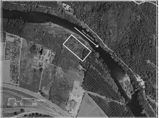
The study reach comprises a 2 km reach of the Ter River (NE Spain) characterised

5

by a low sinuosity meandering river channel morphology, with alternate gravel bars. The channel banks and nearby floodplain areas are stabilised by a dense riparian vegetation, whereas most of the floodplain is occupied by field crops (cereals and alfalfa) and plots with poplar groves. For our purpose, a quadrilateral of 100 m by 50 m from the floodplain area was selected (Fig. 1). The selected area contains an array of

10

vegetation types, including riparian vegetation (with different heights), poplar planted groves and crops.

The initial DEM was generated with LiDAR data (1 point per m2), previously classified as ground data using the TerraScan software (Terrasolid, 2001). Ground points were then interpolated into a raster model of 1 m cell size. A low pass filter was used to

15

generalise the model and to remove or to reduce local detail. The “low pass” filter operates by moving a window of 3_×3 across the entire raster and the new value for the cell at the middle of the window is a weighted average of the values in the window. The resultant DEM was a smoothed generalised version of the topographic surface for a mesh resolution of 1 m (referred to as DEMref). LiDAR elevation points were

20

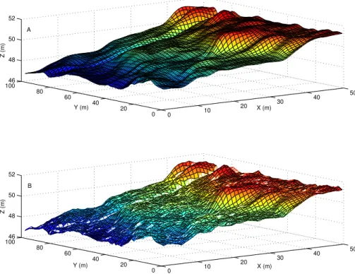
progressively added to increase the amount of topographic complexity to DEMref (i.e. more LiDAR elevation points). This is achieved using a vertical variability threshold criterion (see Fig. 2a), i.e. when the distance between the reference DEM (Fig. 3a) and the point to be added is within the vertical (e.g._±25 cm) threshold, the point is selected to be incorporated in the DEM (e.g. DEM_±25 cm), (Fig. 3b). Four vertical variability

25

(7)

HESSD

7, 2261–2299, 2010

A. Casas et al.

Title Page

Tables Figures

◭ ◮

Back Close

Full Screen / Esc

as measured in the original LiDAR data. The sampled data were combined with the data in DEMref to create a Topographical Irregular network (TIN) structure that was then interpolated into a raster model of 1m mesh cell size. Therefore, five DEMs are generated, the reference one (DEMref) and four with additional topographic content (_±∆z), DEM±5cm, DEM±10cm, DEM±25cm, DEM±50cm(Casas et al., 2010). These DEMs

5

have different topographic contents, the increase of the vertical threshold of LiDAR data will produce DEMs with higher vertical variability which can be quantified using spatial statistics. In this study, the semivariance and Geary’s C spatial autocorrelation index are used.

2.2 Roughness parameterisation

10

LiDAR-derived roughness height (z0) values for each cell of the modelled surface

per-mits an objective estimation of the flow resistance for each cell of the 2-D floodplain inundation model. This study uses a new mixing layer theory for flow resistance in shallow streams developed by Katul et al. (2002). This approach predicts flow resis-tance from surface roughness measures and water depth using a mixing layer analogy

15

rather than the standard rough-wall boundary layer theory. The mixing layer theory with its inflectional profile yields mean flow velocities at high relative roughness, providing analytical linkage between depth, roughness, and velocity forh/z0<7 wherehis water

depth andz₀roughness height.

The approach makes use of the turbulent flow structure within and above rigid

veg-20

etation canopies. The structure of the flow near extensive and porous roughness ele-ments resembles a mixing layer with an inflection near the mean height of the rough-ness element (D), Fig. 4, (Raupach et al., 1996 cited by Katul et al., 2002) whereas rough-wall boundaries do not possess an inflection point (Katul et al., 2002).

The theory acknowledges that the mean velocity within the roughness element is

25

(8)

pro-HESSD

7, 2261–2299, 2010

A. Casas et al.

Title Page Abstract Introduction Conclusions References Tables Figures ◭ ◮ ◭ ◮ Back Close

Full Screen / Esc

files are reproduced using a mean velocity equation given by:

U U0

=1+tanh

z₋D

Ls

(1)

whereDis the mean height of the roughness elements;Lsis a characteristic energetic

eddy size (i.e., mixing length) produced atz=D andU0is the mean reference velocity

at z₌D. Following Katul et al. (2002), the depth-averaged velocity can result, for

5

Ls≈αD:

U u₀ =

1

h Zh

0

1+tanh

z₋D

αD

d z=1+αD

h ln

cosh _α1₋_αDh

cosh 1_α !

(2)

By letting:u0=Cuu_∗;ξ=Dh;

f(ξ,α)=1+α1 ξln

cosh _α1₋_αhξ

cosh _α1 !

(3)

It can be expressed as :

10

U

u_∗ =Cuf(ξ,α) (4)

whereC_u is a similarity constant andu_∗is the friction velocity:

u_∗=

q

ghS (5)

where S is the bed slope andhthe depth

The result in Eq. (4) is highly dependent on the definition of D. Upon comparing

15

Eqs. (4), (5) and Manning’s equation for a wide rectangular channel:

U=1

nh

2

(9)

HESSD

7, 2261–2299, 2010

A. Casas et al.

Title Page

Tables Figures

◭ ◮

Back Close

Full Screen / Esc

a relation between the depth-averaged velocity and Manning’sncan be explicitly es-tablished:

n= h

1 /6

√_gC

uf(ξ,α)

(7)

Values ofα=1 andCu =4.5 are recommended for a range ofh/Dof between 0.2 and

7.

5

In this study, this equation incorporated into the 2-D flood model and a roughness value is obtained for each cell of the domain at every time step of the calculation. The mean height of the roughness element (D) is set to be the averaged value of the roughness height (z₀) data located within a cell of the model mesh, where z₀ is cal-culated as the difference between the DEM and measured LiDAR point, (see Fig. 2b).

10

Thus, the definition ofD, and thereforen, will depend upon the mesh resolution of the scheme. Therefore, the modelling scheme of the 2-D hydraulic model applied in this study requires a Digital Roughness Model (DRM) with D values as the mean height of the roughness heights (z0) contained within the cell (see Fig. 2b). The DRM at

a given mesh resolution, along with the local water depth are required to provide a

15

spatio-temporally varying parameterisation of surface friction in the flood model. The methodology developed in this study to obtain a distributed roughness parame-terisation is based on roughness height information (z0) of non-terrain elements derived

from LiDAR points recorded but not classified and thus not included in the terrain model generation as topographic content (∆z), (see Fig. 2a). Therefore, using this scheme,

20

roughness height (z0) estimation will be dependent on the topography used to

gener-ate the DEM and its mesh resolution. Where the DEM does not represent topography explicitly, the model accounts for it through the roughness height (z0).

Roughness height calculation uses LiDAR altimetric data to which the elevation of the DEM is subtracted using a GIS routine (e.g. Cobby et al., 2001). The resultant

25

roughness height (z0), which is the measured LiDAR data detrended from the terrain

(10)

HESSD

7, 2261–2299, 2010

A. Casas et al.

Title Page

Tables Figures

◭ ◮

Back Close

Full Screen / Esc

the DEM into a DRM.

In this approach, it is assumed that the laser measures the range to any obstacle which subsequently disturbs the flow pattern at a specific location. Thus, momentum roughness height (z0 or the height at which velocity becomes zero) is considered to

be the difference between the height at which the laser find the higher physical solid

5

obstacle and the estimated terrain height at that location.

2.3 Hydraulic modelling

In this study, a hybrid 1-D–2-D hydraulic model (FloodMap) of flood inundation has been used. FloodMap (Yu and Lane, 2006a, b) is a coupled 1-D/2-D flood inundation model designed for fluvial flood inundation prediction in topographically complex

flood-10

plains. It has a similar structure to that of JFLOW (Bradbrook et al., 2004). The model is the basis of the sub-grid treatment approach developed by Yu and Lane (2006b) and FloodMap-Parallel (Yu, 2010). It has been tested and verified with a range of boundary conditions and in a number of environments (Yu, 2005; Tayefi et al., 2007; Lane et al., 2007, 2008). Yu and Lane (2006a) have reviewed the basis of the model,

15

and so only the major model structure is outlined here. The coupled model assumes that the floodplain is protected by an embankment that essentially acts as a con-tinuous, broad-crested weir through which flow exchange occurs between the chan-nel and floodplain. A tightly-coupled approach solves the one-dimensional river flow and two-dimensional floodplain flows simultaneously in a raster environment. The

20

one-dimensional in-channel model solves the full Saint-Venant equations for unsteady open-channel flow using the Preissmann scheme based upon the fixed bed model of Abbott and Basco (1989).

The floodplain flow is simulated with a 2-D diffusion-based approach based on the discretisation of the Manning’s equation in a raster-based environment. The model

25

(11)

HESSD

7, 2261–2299, 2010

A. Casas et al.

Title Page

Tables Figures

◭ ◮

Back Close

Full Screen / Esc

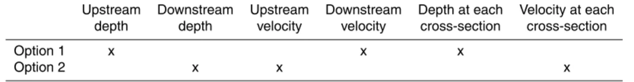
2.3.1 Model boundary conditions

Three types of boundary conditions are required by the 1-D component of FloodMap, i.e. upstream and downstream flow hydrographs, river cross sectional geometry, and roughness parameter in each cross section. In terms of the flow boundary conditions, FloodMap can use a combination of either: (i) velocity upstream and stage

down-5

stream; or (ii) velocity downstream and stage upstream. In addition: (i) requires the velocity at each cross-section at the start point of simulation; and (ii) requires the wa-ter depth at each cross-section at the start of simulation, as initialisation data. This is summarized in Table 1. For this application, the second option is used.

There were no measured flow boundary conditions available at the domain boundary

10

of the study site to initialize the 1-D component of FloodMap. Instead, these were ob-tained from a one-dimensional hydraulic HEC-RAS model (Reference of Army Corps of Engineers) implemented along a 2 km long river reach run for subcritical flow con-ditions (Casas et al., 2006). The associated water depth and velocity used here are shown in Table 2. For this reach, the flow boundary conditions required by FloodMap

15

were calculated with an initial discharge of 25 m3s−1.

A simple cross section geometry of a rectangular shape is used in this study. For each cross-section, channel width and depth are required to represent the cross sec-tion geometry. These were calculated with cross-secsec-tion GPS coordinates obtained from field survey. For the 1-D model, Manning’sncoefficients at each cross section at

20

the simulation domain were obtained through a calibration process from the HEC-RAS modelling (Casas et al., 2006). In total thirteen cross sections were used in the study site. The associated boundary conditions required by the model are shown in Table 3. These boundary conditions are introduced in the model as ASCII files.

The model was run for the whole floodplain area for each DEM and the associated

25

(12)

HESSD

7, 2261–2299, 2010

A. Casas et al.

Title Page

Tables Figures

◭ ◮

Back Close

Full Screen / Esc

2.4 Characterisation of topography and modelled flow fields

The level of organisation of the DEMs and simulated flow according to the topographic content or the roughness parameterisation is quantified using spatial statistics. The semivariance statistic which uses the squared differences between neighbouring pixel values provide an idea of the vertical variability underlying each surface for a certain

5

lag. A lag of 1 pixel has been selected as it is the mesh resolution of DEMs, therefore each pixel is evaluated against its immediate neighbour. Semivariance values quantify the increment in the variability of the DEM as the vertical threshold∆zof input data are increased (i.e. its topographic content)

Spatial autocorrelation, using Geary’s C index, has also been calculated for the

10

scaled DEMs to quantify the homogeneity in the spatial pattern of each DEM through the comparison of neighbouring pixel values. Geary’s C uses the formula:

C(d)=

(n₋1)

n

P

i n

P

j

wi j yi−yj

2

2W

n

P

i

z2_i

(8)

Wherew_{i j} is the weight at distanced,z’s are deviations from the mean for variabley, andW is the sum of all the weights wherei 6=j. The value ranges from 0.0 to 3.0, with

15

0.0 for a strong positive spatial autocorrelation and+1 for no correlation. Values from 1.0 to 3.0 indicate negative correlation.

3 Results

Firstly, the distributed roughness parameterisation methodology developed is evalu-ated and the topographic content of DEMs is quantified. Secondly, scaling e_ffects

20

(13)

HESSD

7, 2261–2299, 2010

A. Casas et al.

Title Page

Tables Figures

◭ ◮

Back Close

Full Screen / Esc

topographic content of the DEM are assessed. Thereafter, the topographic content im-pact is isolated and the level of organisation of depth results is quantified through the Geary’s C spatial autocorrelation index (Eq. 8). Finally, the full area is considered and model results are evaluated.

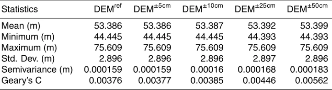
Descriptive statistics and semivariance values for each DEM are summarized in

Ta-5

ble 4. Semivariance values increase as the models comprise more topographic con-tent for a fixed mesh resolution. In addition, the spatial autocorrelation Geary’s C index (Eq. 8) has been calculated to compare the homogeneity between these DEMs as to-pographic content is introduced. Table 4 shows that Geary’s C spatial autocorrelation index decreases as larger topographic content is introduced.

10

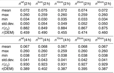
Table 5 summarises the statistics of roughness parameterisation (n, from Eqs. 2 and 3) for the 2nd and 4th h of the simulation according to each scaled scheme for the detailed studied floodplain area. The Table shows that the Manning’snparameter does not vary systematically with any of scaled schemes but according to an interaction between topography and, therefore, depth and roughness height. As expected, the

15

mean roughness parameter, and its standard deviation, decreases from the second hour to the fourth hour. It must be noted that these scaled topographies are constructed for a constant mesh resolution which is known to have a large impact in this kind of hydraulic models (e.g. Yu and Lane, 2006a).

Figure 6 shows, for the detailed studied floodplain area (Fig. 1), the input data

(rough-20

ness heights (Fig. 6a) and model derived depths (Fig. 6b) required to calculate the

distributed roughness parametern (Fig. 6c). Roughness heights and roughness

pa-rameter are correlated (Fig. 6) where Manning’sn values vary from 0.036 to 0.25 for a range of 0.02–5.6 m of roughness heights. This is confirmed in Table 5 where corre-lation coefficient (r) of Manning’snparameter in relation to roughness height (z0) and

25

topographic elevation (DEM) is calculated as a measure of the agreement between model components.

(14)

HESSD

7, 2261–2299, 2010

A. Casas et al.

Title Page

Tables Figures

◭ ◮

Back Close

Full Screen / Esc

different topographic content (_±∆z) can be assessed for our detailed floodplain area (see Fig. 1). Figure 7 represents the impact (RMSD) on roughness parameterisation (Fig. 7a) and depth derived results (Fig. 7b) for a detailed floodplain area at the 2nd and 4th h of the simulation. The impact of additional subscale complexity (_±5,_±10,_±25 and ±50) in the model upon both roughness parameterisation and depth derived results

de-5

creases towards the 4th h (Fig. 7). Figure 7a shows the comparison (RMSD) between roughness parameterisations obtained using Eq. (7). It suggests that the impact is not systematic with the linear increment of the topographic subscale complexity that results from variation in the topographic content of the DEM and roughness height. Therefore, the roughness parameterisation model is sensitive to interactions between distributed

10

roughness height and topographic content. The distributed scale-dependent method-ology comprises the interaction between topography and roughness. Figure 7b shows, the comparison (RMSD) between flow depth results using models with additional sub-scale complexity (_±5,_±10,_±25 and_±50) with those obtained using a reference one without additional complexity (ref). The figure shows that the impact is not

system-15

atic with the linear increment of the topographic subscale complexity. However, from the comparison of Fig. 7a and b, it can be noted that variations (RMSD) in flow depth results are systematic with variations (RMSD) in roughness parameterisation.

The percentages of the normalised differences of the depth derived results using each scaled scheme in relation to the reference one (DEMref) and the Geary’s C

spa-20

tial autocorrelation index have been calculated. Figure 8 shows how, as the spatial

subscale scheme becomes more complex and from±5 cm toward ±50 cm, the

auto-correlation index is closer to 1, which implies lower organisation in the flow. Figure 9 corroborates visually this impact on the structure of the flow, where it is shown how for the subscale scheme (i.e. accounting for more topographic variation at±50 cm) the

25

flow is less organised (Fig. 9a).

(15)

HESSD

7, 2261–2299, 2010

A. Casas et al.

Title Page

Tables Figures

◭ ◮

Back Close

Full Screen / Esc

2nd and 4th h of the simulation. This is calculated for each one of the five simulations with di_fferent topographic content in the DEM. Variations (RMSD) in depth results due to this constant roughness parameterisation are of 0, 0.01, 0.02 and 0.03 when each model (_±5 cm, _±10 cm, _±25 cm, _±50 cm) is compared with the reference one. From these results, it can be stated that for a constant value of roughness height: (i) the

5

roughness parameterisation is not globally sensitive to variations in the topographic content of the DEM; and (ii) the RMSD of depth varies positively, increasing with the increment of topographic content in the 1 m-DEM, though in a very reduce quantity. Therefore, flow variability of the 2-D hydraulic model for a given mesh resolution (close to measured topographic resolution) relies upon the interactions between topographic

10

variability (_∆z) and roughness parameterisation (n), the former with a stronger and non-linear impact.

Depth derived results obtained using a distributed roughness parameterisation have been compared (RMSD) with those model results obtained using the same roughness parameterisation methodology but a constant roughness height (Fig. 10). Figure 10

15

shows that the impact (RMSD) of using a constant or a distributed roughness param-eterisation according to surface characteristics is larger than the impact of using one topographic model or another (Fig. 7b).

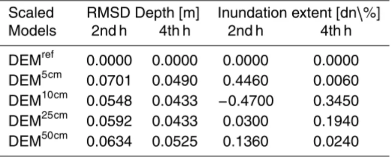
Finally, Table 6 summarises the roughness parameterisation impacts upon depth and inundation extent results at the 2nd and 4th h of the simulation for the full floodplain

20

area. Variations (RMSD and percentage of differences normalised) are compared with the reference simulation results, showing a higher scaling effects on the inundation extent than on depth modelling results

4 Discussion

In river analysis, topography data and hydraulic roughness are major inputs to define

25

terrain geometry.

(16)

topog-HESSD

7, 2261–2299, 2010

A. Casas et al.

Title Page

Tables Figures

◭ ◮

Back Close

Full Screen / Esc

raphy is conceptually accepted, there are fewer studies quantifying the degree of this dependency (e.g. Lane 2005; Horritt 2005). Here we present a method to downscale topography using LiDAR geometric information and to include roughness content with physically meaning criteria.

The blockage impact of downscaled complex topography is incorporated into the

5

hydraulic scheme through a subscale parameterisation. The use of a mixing layer theory for flow resistance has allowed the calculation of a derived roughness parameter at each cell and for each time step of the modelling process. This formulation requires a mean roughness height of the protruding element, which has been calculated using high-resolution LiDAR data not included in the topographic model. This approach has

10

provided a suitable method not only to quantify the roughness properties of the surface but also to test the sensitivity of the hydraulic parameters to a distributed roughness parameterisation approach versus a constant roughness value.

Downscaled analysis shows that variations in flow depth are systematic with varia-tions in the subscale parameterisation and not in relation to the topographic content of

15

the DEM. In fact, when a constant value of roughness height of 0.02 m (bare ground conditions) is applied, the subscale behaviour of the simplified 2-D raster based model is not well-reflected through the topographic content of the DEM. Therefore, subscale flow variations must be modelled through a spatially distributed roughness parameter-isation that can retain small-scale topographic variations within coarse scale models.

20

This implies the convenience of selecting an adequate model scale according to the computing and application demands of the hydraulic model given the low level impact of topographic variability within a certain mesh cell. It also emphasises the importance of including geometric shape details in the hydraulic computation mesh in accordance with some previous studies (Mandlburger et al., 2008; Schubert et al., 2008). This

re-25

(17)

HESSD

7, 2261–2299, 2010

A. Casas et al.

Title Page

Tables Figures

◭ ◮

Back Close

Full Screen / Esc

Our results show that parameterisation process not only influences depth and flood extent but also the structure of the depth derived results. Figure 9 depicts the im-portance of the topographic variability bellow the modelling scale upon the level of organisation of spatially distributed hydraulic results. The main implication of this sub-scale variation upon flow complexity results, according to the complexity of the spatial

5

subscale scheme, is that a distributed subscale parameterisation impacts not only on the range of depth results, as the global RMSD values show, but also modify the char-acteristic scale of flow results. This variation on the level of organisation of modelled flow, as controlled by the down scaled topography at a given mesh resolution, may be important for some ecological applications, such as habitat availability where the river

10

geometry at di_fferent scales plays a decisive role (Hauer et al., 2008; Lane and Carbon-neau, 2007). In addition, this analysis emphasises the need for more comprehensive consideration of the impact of scale on dominant processes and parameter sensitivity (Bates et al., 2005).

The current problem of an appropriate roughness parameterisation is unsolved as,

15

particularly in 2-D schemes, the roughness parameter must account for not only flood-plain vegetation impacts on flow but all momentum losses not explicitly accounted for in the hydraulic model. This fact makes an upscaling necessary although this remains uncertain (Schubert et al., 2008; Straatsma and Baptist, 2008; Horritt et al., 2006; Lane 2005; Mason et al. 2003). Hitherto, the low impacts on flood depths of any

dis-20

tributed roughness parameterisation (e.g. Mason et al., 2007) do not encourage the extra cost of additional multi-spectral data (Straatsma and Baptist, 2008), and also the time demands of featuring a height based resistance scheme to identify flow resistance coefficients and its further model validation with physical realistic values (Schubert et al., 2008).

25

(18)

HESSD

7, 2261–2299, 2010

A. Casas et al.

Title Page

Tables Figures

◭ ◮

Back Close

Full Screen / Esc

of the model in relation to the structure and level of organisation of derived results at the modelling scale. This is important not only to design the modelling scheme but in the validation process. Data chosen to validate a model should reflect what the model must predict (Lane et al., 2005), then the required detailed variability in model results or the spatial structure of available validation data can drive the scale choice of the

5

topographic and roughness parameterisation and should be taken into account in the modelling process.

5 Conclusions

The spatial scale dependency of a 2-D raster-based diffusion-wave model upon to-pographic subscale representation and parameterisation using a distributed spatially

10

and temporally variable roughness parameterisation was assessed. This analysis was based on laser altimetry data (LiDAR) and spatial analysis methods. A methodol-ogy to generate a roughness parameterisation model within the hydraulic model has been developed using down-scaled topographic data. The method explicitly recognises the three-way interaction between the discretised mesh resolution and the topographic

15

content in the DEM with the roughness parameterisation. Subscale parameterisation has been shown to impact depth and inundation extent derived results. Variations in flow results were found to be systematically related to variations in the roughness parameter. The subscale behaviour of the 2-D hydraulic model is not well-reflected through the topographic content of the DEM and subscale parameterisation must be

20

modelled through a spatially distributed roughness parameterisation. Subscale param-eterisation modifies primarily the spatial structure (level of organisation) of simulated 2-D flow linearly with the complexity of subscale parameterisation. There is a clear need to merge these results with variations in the mesh resolution as it may also influ-ence hydraulic modelling results.

(19)

HESSD

7, 2261–2299, 2010

A. Casas et al.

Title Page

Tables Figures

◭ ◮

Back Close

Full Screen / Esc

References

Abbott, M. B. and Basco, D. R. (Eds): Computational fluid dynamics, Longman Scientific and Technical with John Wiley and Sons, New York, USA, 440 pp., 1989.

Ackermann, F.: Airborne laser scanning – present status and future expectations, ISPRS J. Photogramm., 54, 64–67, 1999.

5

Anderson, E. S., Thompson, J. A., Crouse, D. A., and Austin, R. E.: Horizontal resolution and data density effects on remotely sensed LIDAR-based DEM, Geoderma, 132(3–4), doi:10.1016/j.geoderma.2005.06.004, 406–415, 2006.

Antonarakis, A. S., Richards, K. S., and Brasington, J.: Object-based land cover classification using airborne LiDAR, Remote Sens. Environ., 112, 2988–2998, 2008.

10

Antonarakis, A. S., Richards, K. S. and Brasington, J., Bithell, M., and Muller, E.: Retrieval of vegetative fluid resistance terms for rigid stems using airborne LiDAR, J. Geophys. Res., 113, G02S07, doi:10.1029/2007JG000543, 2008.

Asselman, N. E.: Laser altimetry and hydraulic roughness of vegetation – further studies using ground truth, Technical report, Delft, The Netherlands, 84 pp., 2002.

15

Bates, P. D., Marks, K. J., and Horritt, M. S.: Optimal use of high-resolution topographic data in flood inundation models, Hydrol. Process., 17, 537–557, 2003.

Bates, P. D., Lane, S. N., and Ferguson, R. I.: Computational Fluid Dynamics modelling for environmental hydraulics, in: Computational Fluid Dynamics Applications in Environmental Hydraulics, edited by: Bates, P. D., Lane, S. N., and Ferguson, R. I., John Wiley and Sons

20

Ltd, 1–15, 2005.

Bradbrook, K. F., Lane, S. N., Waller, S. G., and Bates, P.: Two dimensional diffusion wave modelling of flood inundation using a simplified channel representation, Journal of River Basin Management, 2(3), 1–13, 2004.

Casas, A., Benito, G., Thorndycraft, V. R., and Rico, M.: The topographic data source of digital

25

terrain models as a key element in the accuracy of hydraulic flood modelling, Earth Surf. Proc. Land., 31(4), 444–456, 2006.

Casas, A., Lane, S. N., Hardy, R. J., Benito, G., and Whiting, P. J.: Reconstruction of subgrid-scale topographic variability and its effect upon the spatial structure of three-dimensional river flow, Water Resour. Res., 46, W03519, doi:10.1029/2009WR007756, 2010.

30

(20)

HESSD

7, 2261–2299, 2010

A. Casas et al.

Title Page

Tables Figures

◭ ◮

Back Close

Full Screen / Esc

review, 2010.

Cobby, D. M., Mason, D. M., and Davenport, I. J.: Image processing of airborne scanning laser altimetry for improved river flood modelling, ISPRS J. Photogramm., 56(2), 121–138, 2001. Cook, A. and Merwade, V.: Effect of topographic data, geometric configuration and modeling

approach on flood inundation mapping, J. Hydrol., 377, 131–142, 2009.

5

Doneus, M. and Briese, C.: Digital terrain modelling for archaeological interpretation within forested areas using full-waveform laserscanning, in: The 7th International Symposium on Virtual Reality, Archaeology and Cultural Heritage VAST, edited by: Ioannides, M., Arnold, D., Niccolucci, F., and Mania, K., Zypern, 3612–3613, 2006.

Gomes-Pereira, L. M. and Wicherson, R. J.: Suitability of laser data for deriving

geograph-10

ical information: a case study in the context of management of fluvial zones, ISPRS J.Photogramm., 54(2–3), 105–114, 1999.

Gueudet, D.: The influence of post-spacing density of DEMs derived from LiDAR on flood modeling, Technical report, University of Texas at Austin, USA, 119 pp., 2004.

Haile, A. T. and Rientjes, T. H. M.: Effects of LiDAR DEM resolution in flood modelling: A

15

model sensitivity study for the city of Tegucigalpa, Honduras, in: ISPRS WG III/3, III/4, V/3 Workshop “Laser scanning 2005”, Enschede, The Netherlands, 2005.

Hauer, C., Mandlburger, G., and Habersack, H.: Hydraulically related hydro-morphological units: description based on a new conceptual mesohabitat evaluation model (MEM) using LiDAR data as geometric input, River Res. Appl., 25, 29–47, 2009.

20

Hirata, Y.: The effects of footprint size and sampling density in airborne laser scanning to extract individual trees in mountainous terrain, International Archives of Photogrammetry, Remote Sensing and Spatial Information Sciences, 36(8), 102–107, 2004.

Hodgson, M. E. and Bresnahan, P.: Accuracy of airborne LiDAR-derived elevation: Empirical assessment and error budget, Photogramm. Eng. Rem. S., 70(3), 331–339, 2004.

25

Horritt, M. S.: Parameterisation, validation and uncertainty analysis of CFD models of fluvial and flood hydraulics in the natural environment, in: Computational Fluid Dynamics Applica-tions in Environmental Hydraulics, edited by: Bates, P. D., Lane, S. N., and Ferguson, R. I., John Wiley and Sons Ltd, 193–213, 2005.

Horritt, M. S., Bates, P. D., and Mattinson, M. J.: Effects of mesh resolution and topographic

30

representation in 2-D finite volume models of shallow water fluvial flow, J. Hydrol., 329, 306– 314, 2006.

(21)

HESSD

7, 2261–2299, 2010

A. Casas et al.

Title Page

Tables Figures

◭ ◮

Back Close

Full Screen / Esc

resistance in shallow streams, Water Resour. Res., 38(11), 1250–1250, 2002.

Lane, S. N., Hardy, R. J., Elliott, L., and Ingham, D. B.: Numerical modeling of flow processes over gravelly surfaces using structured grids and a numerical porosity treatment, Water Re-sour. Res., 40, W01302, doi:10.1029/2002WR001934, 2004.

Lane, S. N.: Roughness-time for a re-evaluation?, Earth Surf. Proc. Land., 30, 251–253, 2005.

5

Lane, S. N., Hardy, R. J., Ferguson, R. I., and Parsons, D. R.: A framework for model verifica-tion and validaverifica-tion of CFD schemes in natural open channel flows, in: Computaverifica-tional Fluid Dynamics Applications in Environmental Hydraulics, edited by: Bates, P. D., Lane, S. N., and Ferguson, R. I., John Wiley and Sons Ltd, 169–192, 2005.

Lane, S. N. and Ferguson, R. I.: Modelling reach-scale fluvial flows, in: Computational Fluid

10

Dynamics Applications in Environmental Hydraulics, edited by: Bates, P. D., Lane, S. N., and Ferguson, R. I., John Wiley and Sons Ltd, 217–269, 2005.

Lane, S. N., Tayefi, V., Reid, S. C., Yu, D., and Hardy, R. J.: Interactions between sediment delivery, channel change, climate change and flood risk in a temperate upland environment, Earth Surf. Proc. Land., 32(3), 429–446, 2007.

15

Lane, S. N. and Carboneau, P. E.: High resolution remote sensing for understanding instream habitat, in: Hydroecology and Ecohydrology, edited by: Wood, P. E., Hannah, D. M., and Sadler, J. P. Wiley & Sons, Ldt, 185–204, 2007.

Lane, S. N., Reid, S. C., Tayefi, V., Yu, D., and Hardy, R. J.: Reconceptualising coarse sediment delivery problems in rivers as catchment-scale and diffuse, Geomorphology, 98, 227–249,

20

2008.

Leclerc, M.: Ecohydraulics. A new interdisciplinary frontier for CFD, in: Computational Fluid Dynamics Applications in Environmental Hydraulics, edited by: Bates, P. D., Lane, S. N., and Ferguson, R. I., John Wiley and Sons Ltd, 429–460, 2005.

Liu, X.: Airborne LiDAR for DEM generation: some critical issues, Prog. Phys. Geog., 32(1),

25

31–49, 2008.

Mandlburger, G. and Briese, C.: Using Airborne Laser Scanning for Improved Hydraulic Models, in: International Congress on Modelling and Simulation, 731–738, 2007.

Mandlburger, G., Hauer, C., H ¨ofle, B., Habersack, H., and Pfeifer, N.: Optimisation of LiDAR derived terrain models for river flow modelling, Hydrol. Earth Syst. Sci., 13, 1453–1466,

30

2008,

http://www.hydrol-earth-syst-sci.net/13/1453/2008/.

(22)

HESSD

7, 2261–2299, 2010

A. Casas et al.

Title Page

Tables Figures

◭ ◮

Back Close

Full Screen / Esc

flow models, Hydrol. Process., 14, 2109–2122, 2000.

Mason, D. C., Horritt, M. S., Hunter, N. M., and Bates, P. B.: Use of fused airborne scanning laser altimetry and digital map data for urban flood modelling, Hydrol. Process., 21, 1436– 1447, 2007.

Mason, D. C., Cobby, D. M., Horritt, M. S., and Bates, P. D.: Floodplain friction

parameteri-5

zation in two-dimensional river flood models using vegetation heights derived from airborne scanning laser altimetry, Hydrol. Process., 17, 1711–1732, 2003.

Menenti, M. and Ritchie, J. C.: Estimation of effective aerodynamic roughness of walnut gulch watershed with laser altimeter measurements, Water Resour. Res., 30 (5), 1329–1337, 1994.

10

Nicholas, A. P.: Roughness parameterization in CFD modelling of gravel-bed rivers, in: Com-putational Fluid Dynamics Applications in Environmental Hydraulics, edited by: Bates, P. D., Lane, S. N., and Ferguson, R. I., John Wiley and Sons Ltd, 329–355, 2005.

Omer, C. R., Nelson, E. J., and Zundel, A. K.: Impact of varied data resolution on hydraulic modelling and floodplain delineation, J. Am. Water. Resour. As., 39 (2), 467–475, 2003.

15

Poggi, D. and Katul, G. G.: The effect of canopy roughness density on the constitutive compo-nents of the dispersive stresses, Exp. Fluids, 45, 111–121, doi:10.1007/s00348-008-0467-7, 2008.

Poggi, D., Krug, C., and Katul, G. G.: Hydraulic resistance of submerged rigid veg-etation derived from first-order closure models, Water Resour. Res., 45, W10442,

20

doi:10.1029/2008WR007373, 2009.

Popescu, S. C. and Zhao, K.: A voxel-based LiDAR method for estimating crown base height for deciduous and pine trees, Remote Sens. Environ., 112, 767–781, 2008.

Raber, G.: The effect of LiDAR posting density on DEM accuracy and flood extent delineation. A GIS-simulation approach, Technical report, 34 pp., 2003.

25

Schubert, J. E., Sanders, B. F., Smith, M. J., and Wright, N. G.: Unstructured mesh generation and landcover-based resistance for hydrodynamic modeling of urban flooding, Adv. Water Resour., 31, 1603–1621, 2008.

Straatsma, M. W. and Middelkoop, H.: Airborne laser scanning as a tool for lowland floodplain vegetation monitoring, Hydrobiologia, 565, 87–103, 2006.

30

(23)

HESSD

7, 2261–2299, 2010

A. Casas et al.

Title Page

Tables Figures

◭ ◮

Back Close

Full Screen / Esc

Suarez, J. C., Ontiveros, C., Smith, S., and Snape, S.: Use of airborne LiDAR and aerial photography in the estimation of individual tree heights in forestry, Geospatial Research in Europe: AGILE 2003, Comput. Geosci., (31)2, 253–262, doi:10.1016/j.cageo.2004.09.015, 2005.

Tayefi, V., Lane, S. N., Hardy, R. J., and Yu, D.: A comparison of 1-D and 2-D approaches

5

to modelling flood inundation over complex upland floodplains, Hydrol. Process., 21, 3190– 3202, 2007.

Terrascan user’s guide: http://www.terrasolid.fi, 2001.

Wehr, A. and Lohr, U.: Airborne laser scanning – an introduction and overview, ISPRS J. Photogramm., 54, 68–82, 1999.

10

Yu, D.: Two-dimensional diffusion wave modelling of structurally complex floodplains, Ph.D. thesis, University of Leeds, UK, 240 pp., 2005.

Yu, D. and Lane, S. N.: Urban fluvial flood modelling using a two-dimensional di_ffusion-wave treatment, part 1: mesh resolution e_ffects, Hydrol. Process., 20(7), 1541–1565, 2006a. Yu, D. and Lane, S. N.: Urban fluvial flood modelling using a two-dimensional diffusion-wave

15

treatment, part 2: development of a sub-grid-scale treatment, Hydrol. Process., 20 (7), 1567– 1583, 2006b.

Yu, D: Parallelization of a two-dimensional flood inundation model based on domain decompo-sition, Environ. Model. Softw., doi:10.1016/j.envsoft.2010.03.003, 2010.

(24)

HESSD

7, 2261–2299, 2010

A. Casas et al.

Title Page

Tables Figures

◭ ◮

Back Close

Full Screen / Esc

Table 1.Boundary condition requirements for the 1-D river model. (Option 2 is used in this study).

Upstream Downstream Upstream Downstream Depth at each Velocity at each depth depth velocity velocity cross-section cross-section

Option 1 x x x

(25)

HESSD

7, 2261–2299, 2010

A. Casas et al.

Title Page

Tables Figures

◭ ◮

Back Close

Full Screen / Esc

Table 2.Inflow data.

Time Discharge Depth (m) Velocity (m s−1) (h) (m3s−1) downstream upstream

(26)

HESSD

7, 2261–2299, 2010

A. Casas et al.

Title Page

Tables Figures

◭ ◮

Back Close

Full Screen / Esc

Table 3.Model geometry and boundary conditions estimated for an initial discharge of 25 m3s−1.

width length bed elevation Manning’s mean velocity depth XS-ID (m) (m) (m) n (m2s−1) (m)

(27)

HESSD

7, 2261–2299, 2010

A. Casas et al.

Title Page

Tables Figures

◭ ◮

Back Close

Full Screen / Esc

Table 4.Descriptive statistics for each scaled DEM.

(28)

HESSD

7, 2261–2299, 2010

A. Casas et al.

Title Page

Tables Figures

◭ ◮

Back Close

Full Screen / Esc

Table 5. Statistics of roughness parameter (n) due to variations in the topographic content of the DEM (∆z) and the roughness height (z₀) of the DRM for a detailed area (Fig. 1).

nref(2 h) n5cm(2 h) n10cm(2 h) n25cm(2 h) n50cm(2 h) mean 0.072 0.075 0.072 0.074 0.072 max 0.260 0.259 0.260 0.259 0.260 min 0.034 0.030 0.035 0.033 0.034 std.dev. 0.050 0.054 0.049 0.052 0.050

r(z₀) 0.882 0.849 0.884 0.867 0.875

r(DEM) 0.459 0.490 0.455 0.474 0.460

nref(4 h) n5cm(4 h) n10cm(4 h) n25cm(4 h) n50cm(4 h) mean 0.067 0.068 0.067 0.068 0.067 max 0.260 0.260 0.259 0.260 0.260 min 0.038 0.037 0.038 0.038 0.038 std.dev. 0.041 0.043 0.041 0.042 0.041

(29)

HESSD

7, 2261–2299, 2010

A. Casas et al.

Title Page

Tables Figures

◭ ◮

Back Close

Full Screen / Esc

Table 6. Scaling effect upon depth derived results (RMSD) and inundation extent (differences normalised %) due to subscale parameterisation for the full area at the 2nd and 4th h of the simulation, compared with the reference model (DEMref_1m) simulation results.

(30)

HESSD

7, 2261–2299, 2010

A. Casas et al.

Title Page

Tables Figures

◭ ◮

Back Close

Full Screen / Esc

(31)

HESSD

7, 2261–2299, 2010

A. Casas et al.

Title Page

Tables Figures

◭ ◮

Back Close

Full Screen / Esc

±25cm

LiDAR

point

DEM

±25cm

DEM

ref

(A)

Z

₀ref

Z

0±25cm

LiDAR

points

DEM

ref

(B)

Z

0ref

Z

₀ref

D

ref

(32)

HESSD

7, 2261–2299, 2010

A. Casas et al.

Title Page

Tables Figures

◭ ◮

Back Close

Full Screen / Esc

0 10

20 30

40 50

0 20 40 60 80 10046

48 50 52

X (m) Y (m)

A

Z (m)

0 10

20 30

40 50

0 20 40 60 80 10046

48 50 52

X (m) Y (m)

B

Z (m)

(33)

HESSD

7, 2261–2299, 2010

A. Casas et al.

Title Page

Tables Figures

◭ ◮

Back Close

Full Screen / Esc

(34)

HESSD

7, 2261–2299, 2010

A. Casas et al.

Title Page

Tables Figures

◭ ◮

Back Close

Full Screen / Esc

Interactive Discussion 0

10

20

30

40

50

0 20 40 60 80 100

0 1 2 3 4 5 6 7

(35)

HESSD

7, 2261–2299, 2010

A. Casas et al.

Title Page

Tables Figures

◭ ◮

Back Close

Full Screen / Esc

Value

High : 0.249129

Low : 0.035505

Value

High : 5.571127

Low : 0.020000

A C

Value

High : 7.342600

Low : 0.283500 B

(36)

HESSD

7, 2261–2299, 2010

A. Casas et al.

Title Page

Tables Figures

◭ ◮

Back Close

Full Screen / Esc

(37)

HESSD

7, 2261–2299, 2010

A. Casas et al.

Title Page

Tables Figures

◭ ◮

Back Close

Full Screen / Esc

(38)

HESSD

7, 2261–2299, 2010

A. Casas et al.

Title Page

Tables Figures

◭ ◮

Back Close

Full Screen / Esc

%dn±10cm %dn±5cm

%dn±25cm %dn±50cm

(A) (B) (C) (D)

(39)

HESSD

7, 2261–2299, 2010

A. Casas et al.

Title Page

Tables Figures

◭ ◮

Back Close

Full Screen / Esc