Income and demand policies in Brazil

I I I

N9 129

FINANCIALDEEPENING IN BRAZIL _. '

CAPITULO ·111

INCOME ANO OEMANO POLICIES IN BRAZIL Rubens Penha Cysne

Setembro de 1988

INCOME AND DEMAND POLICIES IN BRAZIL

Rubens Penha Cysne*

September, 1988

Revised Version

CHAPTER III

INCOME AND DEMAND POLICIES IN BRAZIL

Introduction

This chapter is divided into four sections. In the . first,

are presented three different ways to ccrrect t-he continuous loss of purchasing

power of wages in an inf1ationary environment. lqe concentrate our

attention on the two mechanisms that have been used in Brazi1: The

"peak adjustment" and the "average adjustment". In the former case,

wages are corrected taking into consideration on1y past inf1ation

In the latter, future inf1at.ion mt1.st be forecasted to

perrnit the ca1cu1ation of the nominal wage adjustment necessary to

keep its purchasing power at the previous prevai1ing va1ue. These

different methodo1ogies 1ead to comp1etely different sitúations with

respect to combating inflation, and are a key step in understarrl in the

inflationary process in Brazil. The "peak adjustment" is generally

referred to in the 1iterature as lagged (backward looking) indexation

The "average adjustment" is better defined as an income po1icy than

as a method to index wages. It is also satetiIres referred to as " fo:rward looking ｪｮ､･ｸ｡ｴｩｯｩｾ＠

'lhe "average adjustment ", which presents an additiona1

degree of freedom for policy-makers trying to combat inf1ation,

was the basic too1 used to bring year1y inflation down fram 91,9% to

24,9% in the :p=riod 1964 to 1967 (under the PAEG Plan). This was the only successful attempt to combat high rates of inflation (for

brazi1ian standards, high rates shou1d be defined as above 40% a

year) in Brazil. The extent to which inflation was reduced finds no

para1'le1 in the economic history of the country. A second attempt to

.2.

stabilize the 226% average inflation rates prevailing between 1983

and 1985, was given by the Cruzado Plan, launched on February, 28,

1986. However the lack of adequate demand controls led to a

complete disaster. Section 2 is dedicated to the description and

comparison of these two attempts towards price stabilization (PAEG

and Cruzado Plans) .

Section 3 concentrates on the complicated institutional relationships between the Federal Treasury, Central Bank of Brazil

and Banco do Brasil, which has led to the existence of two different budgets: the monetary budget and the fiscal budget. The former is

related to the forecasted and approved (by the National Monetary

Council) operating targets of the Central Bank and Banco do Brasil .

Monetary (M_{l ) expansion is pre-determined, and the assets} and

liabili ties ofthese institutions

are

carefully analysed, in order to

make the High Pavered Money expansion compatible with the forecasted evolution of the banking multiplier and the previously determined

expansion rate of Ml (currency plus demand; deposits) The fiscal budget is the offici::ll one, arrl the only

one

subjected to approval of the Congresso It has not been representative of the government

budgetary disequilibrium , though, since many of the expenses of the

Federal Government are' carried out by Bapco do Brasil or the

Central Bank, and directly financed by money supply.

Finally, section 4 concentrates on the consequences over

money demand arising from the continuous process of financiaI

innovations. The econometric estimates presented allow us to

evaluate the magnitude of the autonomous decline in the demand for

real cash balance, which was around 6 % a year sinoe 1964. Particularly,

if the puq:ose is to evaluate the role of Ironetary policy in affecting aggregate

demarrl, this instability of Ironey dernarrl makes it necessary to analyze the

ｉｾＭＭＭＭＭＭＭＭＭＭＭＭＭＭＭＭＭＭＭＭＭＭＭＭＭＭＭＭＭＭＭＭＭＭＭＭＭＭＭＭＭＭＭＭＭＭＭＭＭＭＭＭＭＭＭＭＭＭＭＭＭＭＭＭＭＭＭＭＭＭＭＭＭＭＭＭＭＭＭＭＭＭＭＭＭ

I

.3.

2) Income Policies

Roughly speaking, there are three nain ways to

correct the oontinuous loss of purchasing power of wages due to

inflation. The first, instantaneous indexing, is more easily

described by textbooks than applied in practice. Here, wages are

corrected continuously, and their real value is kept constant

over time. Its approximation in the real world is given by the

triggerpoint methodology: when accumulated inflation since the

last readjustment reaches a certain lirnit, say x%, wages areautanatically

multiplied by I + x/IOO. The lower the value of x' stipulated in

the wage agreements, the lower will be the variation of

real wages.

The main disadvantage of this process, which has been

used already in Italy and Belgien, relies on the fact that the

average purchasing power of labor remuneration in an economy is

not to be considered an exogenous constant,. Indeed, in "periods

of adverse supply shocks, like real exchange rate devaluations,

losses of crops, increase of indirect taxes, decreases of subsidies

or deterioration in the terms of trade, full employment real wages

are naturally supposed to decline. The same thing would happen in

the case of sharp increases of real interest or capital remuneration.

rf the given escalator mechanism does not recognize this fact, as

it would be the case under the trigger point mechanism with low values of inflation to detennine the nominal correction of wages, the

economy becomes subjected to high unemployment rates.

.4.

solely due to supply shocks. But this is not an easy task to achieve.

First, spillover effects make it technically complicated to evaluate

the effect of supply shocks on the price indexo For example, is

hard to say to what extent a loss of production in the orange crop

has affected the price of apples. Second, it is not easy for an

employee to see his wage being a.djusted at a rate belcw the inflation

rate, because of something the economists refer to as "supply shocks".

'lhey do have sorre reason, since positive supply shocks generally do not lead to

wage corrections higher than inflation rates.

AlI of these problems explain why this methodology

was put aside On the aforementioned countries. Overall results

were not positive.

We turn now to the second, and by far the most

popular instrument used in Brazil to replace purchasing power of

wages over time, the so called "peak adjustment" method

The difference between this method and the previously mentioned

("trigger point") one relies on the timing of adjust:.rrent. In the li peak adjustment li case, these dates are determined exogenously and settled ex-ante. 'lhe timing is set arbitrarily. For instance, every six IlDnth or every twelve

IlDnths ma.y te the intervals at which wages are revised. In the case of the

trigger point methodology, these dates are not previously agreed

upon, but endogenously determined by the prevailing rate of

inflation. If it was stipulated that wages were to be adjusted

each tiIre the price leveI increases, for instance, by 10%, the adjustnent will

be quarterly if quarterly inflation 15 10%,or yearly, if yearly inflation is 10%.

An important difference derives from this facto

Under the trigger point methodology, if W stands for the realwage p

_._--_.

---.5.

lowest value the wages can reach before the next adjustment is

given by W /(l+TI), where TI represents the rate of inflation which _p

triggers the new nominal wage revision. If i t was previously settled

that wages would be revised each time inflation reached 10%, the

lowest value of real wages (valley wage, W ) would _v represent a

fraction 10/11 of the peak value. Wi th a uniform rate of inflation,

the average wage would be around 95,4% .of the value existing just

after the last adjustment.

Under the "peak adjustment" methodology, averageanà

valley real wages are a decreasing function of the rate of inflation

occurring between the two pre-settled dates of adjustment. As in

the previous case the valley real wage (W ) _v is a fraction ｬＯＨｬＫｾＩ＠

of the peak real wage. But now the inflation rate in the denominator

is indeterminate, not of a fixed value. It can be one, one hundred or a thousand p3rcent, depending upon the price index path between

the two adjus1:::rrent dates. 'lhe follCMing graph, which presents the evolution of

real wages over tine, helps to understand this issue:

Graph 3.1

Real Wage Evolution in an Inflationary Environrnent

W P

WA

Wv

A

I; /

C' t

:C

_{- - - - peak line}

ri

ｾ＠

___

Ｍｾｾｾ＠

__

ＭＭＭＭＫｾｾｾｾＭＭＭＭＭｾＭＭＭＭＭＭＭＭ average real wage

,

I /

/ -/ / / / , I

!

I /

t-l

/ 1',1

, I

,,' 1

ｾＬＧ＠

I"

/

D - --;'-I -

7

,

,

(,

, I i _i / ＢｾｄＧ＠

I

I I

/ I

t

I

!

I

I

I I,

t+l

_ _ _ _ valley line

.6.

At date t - 1, real wages were brought to the

peak. As time goes on, nominal wages are he1d constant

(up to time t), but prices are continuously rising. This 1eads

to a fall of the purchasing power of wages over time, trans1ated

by the 1ine AB. At time t, real wages reach their lowest value (W ), _v

but are subsequent1y adjusted to the peak (point C in the graph).

'lhis adjust:nEnt is rnade by multip1ying the nominal wages by (1 + TI), where

TI is the inf1ation rate which occurred between dates t - 1 and t.

The average purchasing power of wages between dates

t - 1 and t is proportiona1 to the dashed area below 1ine AB. \'le

show in the appendix that, if the rate of inf1ation is oonstant over

the time period considered, the average real wage(fNA) wi11 be related

to the va1ue (W ) by the formula: _p

TI

(3.1) W A

=

W p. ( I + TI) In ( I + TI)

where TI stands for the inflation which occurred between the dates of wage negotiations. Thus, if wages are adjusted once per year and yearly

infIation is 40%, their average purchasing power will be around 85%

of that existing at the day when they were adjusted.

Expression (3.1) Ieads to the fo11owing

regarding the characteristics of the peak adjustment:

conc1usions

a) The higher the inflation rate, the lower wi11 be

the average-peak ratio (APR) WA/Wpi

b) Given the infIation rate and the term of wage

negotiations (and, consequently, APR), the higher

we bring peak real wages on the adjustrnent ｾｔＧＺｐＮ＠ ｴｾｴＢ＾＠ i"i.'Jht">r wi l' be thei. r averaoe purchasinq

....

.7.

c) Given a certain rate of prices increase, - the

shorter the period of t:irre between wage adjustments, the

higher will be APR.

Equation (1) represents a simple tautology, which,

under certain hipotheses, defines the average value of real wages.

We will see in the next section how this formula had its status

changed in some economic analyses in Brazil, from a tautology to a

theory of inflation, leading to the disastrous cruzado stabilization

Plan, in 1986.

AlI these three facts can be easily understood by

examining graph 3.1 between periods t and t + 1. Line CD _presents

a similar evolution of real wages as existed between periods t - I and t.

It would be the actual one, should the time scheduling of wage

adjustments, the inflation rate,and the peak wage repeat those of

the previcus period. Line CD' shows. what would happen to real wages if inflation were somewhat higher than that existing ｢･ｴｾ＠ periods

t - I and t. Real wages would falI more quicklyand their valley value

would be lower. Also the average real wage would

decline relative to the last period.

Point C' illustrates a possible adjustment above

the peak value. It becomes clear that, given the rate of inflation,

the average real wage would be higher in this case than if the

adjustment had established as a target the peak value l'l •

P

Finally, we rra.ke use of a similar graph to display the

third property of the "peak adjustment" methodology: Given the rate of

inflation, the average peak ratio (APR) is a decreasing function of

- - _____ . _.

__

_________

....-

_______________________ _

.8.

Graph 3.2

Reduction of Wage Indexing Tenn and Increase of lwerage Real Wage

W

- peak value

W A2 _{ｦＭＭＭＭｉＱＭＭｾＭＭＭＭＭ｟ｉ｟ＴＮ｟｟｟ｉＱ｟ｾＭ｟｟ｉＱ｟｟ＭＭＭＭＭＭ} average value (after)

W AI ｦＭＭｾＺＭＭＭｾｾＭＭＭＭＭｉＭＭＭｾｉＭＭＭＭＢＢ＠ .., _ _ _ _ _ _ _ average value (before)

t-l t t+O,5

I I

T - - - ＭｾＭＭ -

-t+l tiIre

With a yearly inflation rate of 40%, for instance,

average real wages will correspond to 84,9% of the peak value if

the indexing term is annual, but 90,7% of the peak value

indexing term is

ｨ｡ｬｦＭｹ･｡ｲｬｹＨｬｾ＠

if the

As can 'be seen, tlle "peak adj ustment" :--methodology

operates as a - severe barrier to any sudden stabilization

of inf1ation. Let us take the brazi1ian case/for instance, in

1985. llie annual inflation rate was 235,1% and wage negotiations were

half-year1y. This is to say that average waqes represented about 75%

of the peak value. Consequently, a sudden drop of inflation rate

to zero wou1d mean that after alI wages had been adj usted according to

the previous peak., there would be a 33% increase of real wages. 'lhis is c1early impossible in the short run, and means that there is no possibility for

(1) If year1y inf1ation is 40% and uniforrn, ha1f-year1y ｩｮｦｬ｡ｴｾｯｮ＠ wi11 be 18,3%. Entering this number in (1) resu1ts W_A = 0,907W

ｉＭｾＭ

.9.

such a stabilization measure to be effective without a change of

incorne policy.

dilenma", is

'lhe solution to this problern, which we call the "averaqe-peak. gi ven by the use of the third rnethod of wage adjustrnents

we are going to present here: the adjustrnent by the average (lIaverage

adjustrnent ll ). The main difference is that the correction ofnorninal

wages is not directed towards the recomposi tion of its peak purmasing prevailing power, but carried out in order to keep unchanged its

average real value in the next period Ｈｬｾ＠ Graph 3.3 _{illustrates this}

rnethodology.

Graph 3.3

The IIAverage Adjustment ll Methodology

Real Nage

A _ _ _ _ ______ ｾ｡ｫ＠ line

______ average line

_ ｾ＠ ________ . __ valley line

B

ｾＭＭＭＭＭＭＭＭＭＭｾＭＭＭＭＭＭＭＭＭＭＭＭｾＭＭＭＭＭＭＭＭＭＭＭＭＭＭｾＭＭＭＭＭＭＭＭＭＭＭＭＭＭＭｾ＠

t-l t (+) tiIre

FollCMing the peak. rnethodology approach, aswe have previously seen, real wages would be brought to point C at time t. Thiswould

also be the adjustment following the lIaverage methodologyll, if

the inflation expected to happen between time t and t + I were equal

(1) A productivity gain can also be added to the prior average, as it was, for

.10.

to that between time t - 1 and time t. Indeed, this would

make the expected average value of real wage·· between dates

t and t

+

1 equal to the previous actual leveI.

But if the objective is to initiate a stabilization plan,

expected inflation for period ｴＨｔｉｾＩ＠ will surely be lower than the previous inflation('TTt _1). Consequent1y, real wages shou1d be brought to a point below C, which we i11ustrate in the graph by CI. If the

actua1 inf1ation really dec1ires as forecasted, average real wages will rernain

the sarre. In the case when expected inf1ation for the next period is zero,

ncmina1 adjustments Irnlst bring real wages to };X)int C". 'Iheir trajectory in

this case would be gi ven by line C" - B", which repeats the average of period t - 1. These points are forma1ized in the

real wage

appendix.

Equation (1) is taken as the basis for formal explanations.

A1though it represents a solution to the APR dilerrma,

the above described methodo1ogy presents a technical chal1enge:

the forecast of future inf1ation. If actual inflation prevailing

as of time t is higher than the predicted one (used to correct wages),

average real wages wi11 turn out to be lower than in the previous

period. A possible way to surpass this difficulty is to base the

wage adjustment to be carried out at date t

+

1 on the average, value

that would have prevailed had inf1ation been correctly

forecasted, and not on the one actually existing. This was

in Brazil between 1968 and 1979.

.11.

2) Two tentatives Towards Stabilization

The solution of the average-peak dilemma by means

of an income policy centered on the "average adjustment" Irethodology

was introduced on two occasions in Brazi1. In the first, during the "Plano de Estabilização do Governo Castello Branco" (PAEG), it was also

accompanied by demand restrictions, and led to a great sucess in

terms of stabilizing inflation. This happened between 1964 and

1966, when inflation fell from 91,9 to 38,2 percent a year.

H<Mever, the seoond attempt was a complete disaster. It happened

in 1986, with the so called "Cruzado Plan". The income policy

was correct, but as ..,Te shall see further in this section,

the easy monetary-fiscal policy destroyed alI possibilities of

achieving any sucesso Only a few months af,ter the beginning of the

plan, alI the efforts t<Mard stabi1ization had been irreversibly 1ost.

The fo11owing tab1e presents some statistics related

to the PAEG p1an:

Table 3.1

Economic Statistics Related to the PAEG P1an

1964 1965 1966

Pub1ic Deficit as _4,0

1,6 1,1

a Percentage of GDP (%)

Monetary (M_l ) Expansion(%) 84,6 76,S 15,8

Inflation(%) (IGP-DI) 91,9 34,5 38,2

GDP Growth ( % ) 2,6 2,1 5,4

Agricultural Sector _{- 1,3 20,1 - 14,6}

Growth (%)

Sources: Conj untura Econânica, Noverrber, 1972.

.12.

As can be ooserved fran the data, in 1964-66 both m::>netary

and fiscal policy were relatively tight. The discrepancy between

the inflation rate and monetary policy in 1965 can be explained

by the decrease of income veloci ty of m::>ney which accarpanies such

stabilization programs. Inflation in the first quarter of 1964

reached 25%, which means by extrapolation, a 144% yearly rate.

From this IX>int of view, the 91,9% rate of inflation at the end of 1964

demonstrated that the plan introduced after March was in the <x>rrect

direction.

Two important facts which helped to tame ihflation

in 1965 were the excellent agricultura 1 crcp an::1 use of the "average adjust:Irent"

ｲｮ･ｾｳｭ＠ to correct minimurn wages in February. Had the peak

adjustment methodology been used, minimurn wages would have been

multiplied by 2,09. Wi th the adjustrnent airned at keeping the average real purchasing paoler equal to the preceding period, minimurn wages were

increased by only 57%. In July, 1965, forward looking indexation was

extended to alI wage negotiations carried out under federal governrrent

influence.

The most cornrnon criticism made about the PAEG plan

was that stabilization was achieved due to the decline - of real

wages. Projected inflation, which was used to correct nominal

wages, was systematically set below actual inflation, leading to

a continuous (in 1965, 1966 and 1967) decline of average purchasing

power of labor remuneration. The situation persisted up to 1968,

when the wage adjustment law was modified.

This criticism applies, not because of the

falI of real wages, but because of the falI of labor income as a

percentage of GDP (measured by Langoni, 1970, p. 163). Indeed, as we

have already mentioned and formally disp1ay in the ｡ｰｾｲｲｬｩｸＬ＠ the decline

·13.

of real wages was to be expected as a natural consequence of the

real exchange rate devaluation, reduction of subsidies, and correc

tion of the prices of public utilities which took place at this

time.

HONever, this was not to irnply a decrease of the labor share in GOP. 'lhis decline shcMs that the burden of stabilization was really biased against enployees. An active policy of increased taxation on capital reventES

arrl decreased taxation on labor inc:x::lrre should have been used to achieve a better sharing of the burdens of adjust:nent bebNeen the two factors of

production.

We should not analyze the PAEG plan only as an

anti-inflationary oriented programo After having inherite:1 a very undesirable

econornic stuation, econorny policy as of the second sernester of

1964 actually layed down the basis for the period of high econornic

growth rates cornrnencing in 1968.

In the period just prior to the introduction of

the PAm plan the econornic situation was chaotic. Inflation rates, besides

being high, were repressed by the many price controls then in operation. The fiscal system was teclmically inconsistente 'lhis adde:1 to the problern of many distortions caused by inflation, such as illusory profits taxation, underesti-mation of depreciation values arrl deliberate delays is making paym:mts by tax

..

payers. Taxation, sorret.i.Iocs, instead of being applied over value added, fell

Up:>n the final value of the product (élB it was the case of the "Imposto de

Ven-das e Consignações I'). 'lhe balance of payments si tuation was also not very cornfortable. An over-valued exchange rate coupled with the absence

of externaI credi t let to systernatic deficits. 'lhe financiaI rnarket

.14.

process of financiaI intermediation, where only previleged investors

could get loans (highly subsidized) from o·fficial insti tutions.

Included among the important achievements attained

between 1964 and 1967 can be rrentioned Lhe folla .. üng (see Simonsen and Campos, 1974):

a) The development of the rronetary correction mecnanism,

which, as we saí,v in Chapter 2, becane an indispensable tool to foster private saving and correct various distortions arising fran inflationi

b) The improvement of the externaI accounts,

represen-ted by the current account surpluses in 1964, 1965 and 1966, as well as by

renewal of the country's ready access to funds borrowed

international financiaI markets;

in the

c) The improvement of the fiscal system. The "Imposto

Sobre Vendas e Consignações", which fell on the final value of

production, was replaced by the "Imposto de Circulação de

Mercado-rias", which was based on value added. Moreover, illusory profi ts

taxation was abolished and monetarily corrected values of the finn's

physical assets began to be used in the detennination of depreciation

values. Fiscal debts postpop-ed by taxpayers nCM were being m:metarily

corrected and some non-functional taxes (as the "imposto do selo")

were abolishedi

d) 'lhe creation of the "Fundo de Garantia de Tempo de Servi-ço" (FGIS) I a lalx>r indemnification system managed by the recently created

"Banco Nacional da Habitação" (BNH). Besides fostering private

savings, this mechanism injected a nevv dynamisn into the labor force. It

provided revenues equalito 8% of the labor expenses of the

and could be withdrawn in case workers lost their jobi

firms

. 15.

(SFH), vJhose main institution was the BNH. Its rrain pUl'"lX)se was to finance

the developn-;::mt of the housing sector. Assets ill1d liabilities of all

institutions affiliated in the SFH were subjected to rronetary correction.

FGTS reserves were included among the SFH's liabilities;

f) The ereation of the Bancos de InvestirrentoandFINN1E,

the former rraJr.ing available long tenn eredi t to investors and the latter dedica ted to finunce the purchasing of national capital gocx:1s.

The other attempt tOvlards stabilization of

inflation based on the "average adjustment" as a solution to the

"average-peak dilemma" was the Cruzado Plan, initiated on February

28, 1986. Contrary to the monetary-fiseal discipline observed between 1964 and 1967, the Cruzado Plan was followed by an easy demand poliey, which undermined any possibility of sueeess.

f.10reover, real wages were not brought to the average (\vhich should

have been the case, since expected inflation was equal to zero), but subjected

to an increase of 8% (and 15% in the case of minimum wages) .

This lack of attention on the demand side was due

to technieal errors as well as political reasons. On thetechnical

side, the accounts related to public expenditures were notelear

enough to allcw the necessary estimates of ､ｩｳｾｵｬｩ｢ｲｩｵｭ＠ in the public finances.

As ex-Planning Minister Delfim Netto once mentioned, "the current annua l i zed public deficit was zero at the first moment,under ealculation one mone1 later,

less than b,-l0 percent of GDP after

erree

months, and more than five percent of

mp

when i t eould not be hidden anymore ". Furtherrrore, the increase of real ta-':

receipts due to the fall of inflation (Oliveira - Tanzi effect) was overestimated.

'lhe fiscal reform earried out three months before the Plan was

introduccd reduced the lags between the generating faetors and

effective tax receipts by the governrnent, at least in the case of

.16.

househo1d income taxo

Besides the 1ack of reliab1e public deficit estimates, which

really made it difficult to rnanage aggregate d2Illand, there seems to have been

a real bias in the overall conception of the Plano 'lhe difficulties associated

with the supply side of inflation \'lere overerTlJ=hasized, anel the demand side was

relegated to second place. With the continuous failure to tame inf1ation by

rreans of monetary fiscal J.X>licy (retween 1979 and 1986), it was SOIrevlhat

out-of--fashion, am:mg the brazilian econanists who were just going to becorre

policy--rnarkers, to present orthodox solutions for the prob1em of inf1ation. M1at the

administrators of economic J.X>licy seem to to ha'..'e forgotten was that, a1though

this concentration tCM7ards eliminating inflationary inertia was _justifiable

refore the beginning of the Plan, when the econcmy was whol1y indexed, it

became dangerous1y misleading after indexation carne to a ha1t. As

a brazi1ian econornist once said; there is "nothing better than a

team of rnonetarists in the governrnent to rnake unorthodox proposals

reasonab1e, and nothing more appropriate than a team of unorthodox

economists in the government to justify orthodox recommendations".

A measure of this bias can be observed in the theory of

"innertia1 inflation", the term the parents of the Cruzado Plan referred to in

describing brazilian inf1ation prevailing at the end of 1985 (1). Inertial

inflation is a term that was in fashion during 1986 arrong brazilian economists.

By this definition, inflation of period t was vmolly explained by inflation of

period t-1. This would be a resu.lt of independent actions of economic agents, who

wou1d try to protect their re1ati ve shares of incorre by increasing prices <md wages, ti11 the point they reached their rraximum prior purchasing pG.ver. F'ormall y , the theory of inertial inflation can be ｩｮｴ･ｾＭｰｲ･ｴ･､＠ as change of status

expression (3.1), v.tüch is changed from a sirrple tauto1ogy into a theory of

inflation,

ai

rreans of the three follCM7ing hypotheses:

from(3.1)

.17.

Hl: Wages are alwuyS readjusted to the, maximum

purchasing power previously reached.

H2: 'The average-peak ratio _l1A/Vlp is a constant.

H3: The period of time between nominal adjustments

can be controlled by the government and is kept

constant.

Gi ven these three

since APR_t

=

APR_t __l ,

hypotheses, it (1) tha t TI t

=

TI t-l .

follows directly

This means that

inflation repeats itself as a consequence of the average-peak

dillemma. Of course the main problem of such a theory of inflation

relies in the assumption that wages are always adjusted to the peak (Hl) , which eliminates the mechanism by means of which controIs

over aggregate demand play an important role in the processo We

will come back to this point.

In the context here presented, inertial inflation

can be defined as the rate of inflation which, in an economy where revenues are readjusted in distinct and pre-established dates aiming at

the highest purchasing power previously reached, keeps oonstant the

average-peak ratio. In other words, it is the inflation rate that

brings real wages to their previous average value.

Before carefully analyzing the validity of the three

hypotheses behind this "theory of inflation", it is of interest to explore this

apparatus, gi ven by (3.1) and Hl, H2, H3. First of all,the inflation

rate will cease to repeat itself each period if anyone of the

three hypotheses Hl, H2, H3 fails to apply. To begin with, let

us take 3n economy wi th yearly revenues adjustments and a 40% annual

.18.

inflation rate. Fran(l), we get APR= 0,85. rf nothing occurs, that is, if IH,

H2 and H3 rerna.in valid in the next perioo, this inflation rate will rereat

i tself to keep APR

=

0,85. Let us develop SOm2 variations around the therre.

First, in item a, we will admit both Hl and H2 to hold, but not H3. The pericd.

of t:i.rre between wage adjustments is supposed to change from one year to a half

year. Second, in item b, we adrnit Hl and H3 to hold, nut not H2. 'lhe average/

reak ratio is admi ttEd to decline due to suppl y shocks. Both examples lead to

different values of the (endogenously determined) inflation rate, which can be

oompatibilized with the brazilian case.

a) The adjustment term is reduced fran twelve (yearly) to six months ＮｾＧｩｔｩｴｨ＠

this change, since the inflation rate TI in (3.1) represents the rate

of change of prices between the adjustm:mt it follo.vs, if Hl and H2

are true, that annual inflation "lill turn out to be half-yearly. Tbis

means that yearly inflation will rise from 40% to 96%«(1,4)2 -1)xlOO%).

This example fits well with the evolution of brazilian inflation in

the eighties. Between 1974 and 1979, inflation was around 40% a year, having jmnped to 101,4% between 1980 and 1982. In November, 1979 incidentally, wage adjustments turned fran annual to half-yearly

which means that the increase of inflation rates was exactly the one necessary to keep unchanged the average-peaJ<. ratio. 'l'ms fact

oorroborates hypotheses H1 and H2 (IU was enforced by the bach-ward

looking indexation) .

b) Due to supp1y shocks (exchange rate deva1uations, indirect tax

increases, 10ss of crops, etc.), the average-reak ratio changes from

0,84 to 0,76, with ha1f-year1y adjustments. Ma]r-ing APR= 0,76 in(3.1),

we get TI

=

80% per serrester or, equivalent1y, 223>,; per year.

anel on ptlrJ:X)se, we used in the examp1e some numbers that

Again

rrakc

equation(3.1) able to get a10ng with the evo1ution of brazilio.n

.19.

a rate aromld 100% per year, inflation jumped to average

223% between 1983 and 1986. Two important factors in this prcx:::ess vlere the agricultural shock in 1982 and. the real

exchange rate devaluation of 1983. Referring to the rrodel

we are dealing VIi th, the rise of inflation would be

explained as necessary to allaw the falI of real wages

resulting frem the aàverse supply shocks. Since APR turn''3d

frem 0,84 to O, 76, the ex-post explanation of inflation is

that real wages had to falI about 9,5 percentage points.

Inflation in this case would be a consequence of supply shocks, coU.?led with a lagged indexation syste.TTI. Of course,

money supply is implicitly considered to be

ｰ｡ｳｳｩｶ･Ｈｬｾ＠

'Ihese two exarrples sha.v that a theory of inflation based on

equation (3.1) arrl on a flexible version of hypotheses Hl, H2 and H3 can be

useful as a complementary tool to understand inflation in an ecooomy subjected

to lagged indexation and an accomodative monetary-fiscal policy.

However, as a theory which predicts that inflation of period t will

exactly repeat inflation of period t - 1 (inertial inflation), it

is extremely poor. The derivation of this proposition from (1)

demands that hypotheses Hl, H2 and H3 are entirely arrl ahlays verified,

obviously an overstatement.

The main problem of the "inertial inflation" theory

is that i t relies on the assurrption that nominal adjustments are alvlays rr.ade

(1) Actually, both up\.;rard shifts in inflation described in items (a) nnd (b) \vere preceded by an incrcase in the rate of monetary expansion in the previous half-year. In the 1979/80 turn, the wagc po1icy change in Novcm-ber 1979 only ratified thc new annual 100% inflation already opcrating si ncc August (making it impossib1c to return to the old 40% a year leveI). In tlw

.20.

in arder to bring real wages i:othe prC:!vious peak of purchasing power. This supposition eliminates Lhe channels by means of which demand controIs affect the path of inflation. Indeed, if the economy i5 subjected to a huge rcCeSSi011 and future rronctary polic..y is supposed to continue tight, it is meaningless to expect that real wages will always and indistinctly be brought to the previous peok.

Even in an economy subjected to lagged indexation, the amplitude of this mechanism is not total. A p&rt of the economy (including new contracts) is always free to translate moderated expectations and unemployment into lower demands for nominal remunerations.

Lagged indexation mechanisms surely give rrore support to the "peak adjustment" hypot.heses OIl), which, as we Sãv-l,constitutes an essential condition for the theory of inertial inflation, Lopes

ＨＱｾＸＶＩ＠ argued thai: indexation was not necessary for HI

to hold. He used Tobin's (1986) criticism of rational expectations models, later formalized by Simonsen(l987), to present analternatlve theoretical background for the " peak adj ustment" hypotheses. Tobin' s

c.; ri ticism was based on the disassociation betvleen each eoonornic agent's

rationality and overall rationali ty. Following this argument, L:Jpes argu2d that cach economic agent could act in a rnanner disassociated fra.'TI otbers,

increasi ng their nominal income (. the role of dem:md was not discussed adequately in the process) in order to replace the previous peak

of purchasing power. The reasoning for this attitude would be the equivalent behaviour he would expect others to follm'l.

Lopes (1983) explicitly recognized that demand peliei could affect the path of inflation. However, following his Phill'·IJS curve estimates, thc product gap cost to be ｰｾｬ､＠ made this option inadvisable. vJhat was not sufficiently tW<.en int0 considcration in the

Cruzado strategy, though, is that .:::fter the beginning of the Plan and

FUNDAÇÃO G:::TÚUO VARGAS

Biblioteca MÓrJn ｾｩＺＺＧＬﾷ＠ ,: ... .". ＬＺ｣［ｴｮｴｙＧｾＺＺＺｮ＠

,

I

the end of indexation, the sensitility of the economy

management was much higher than before.

to

.21.

Contrary to the nccessary emphasis on the

monetary-fiscal policy side, the period during the Cruzado Plan was

characterized by comprehensive and obligatory price controls. The

main objective was not to ｃｏｆｾ｡ｴ＠ inflation through its symptoms,but

to provide the economy with a centralized signaling of what would

be the behaviour of other econom.ic agcnts vii th respect to price setting. Prices \>lere to be controlled for a short period of time (around three

months). HOtlever, things hasppened di.fferently. After the four ini tial

ITDnths, it was not possible to achieve a market equilibrium with the frozen

price leveI and higher incare, and a system of price-premia and black markets

appeared. The ini tial objecti ve of using a price freeze as a way to avoid the

disassociation between individual and general behaviour had gi ven place to a desperate attempt to hide the near collapse of the Cruzado Plan strategy.

The price freeze turned out to be an unfortunate

device during the Cruzado Plano First, because its signaling

function did not work. It was useless to announce that prices would

remain frozen and, at the same time, make an easy fiscal and

monetary policy. Inconsistency is not compatible with credibility.

And credibility is a necessary condition for acting as an orchcstra

conductor. Second, the price freeze led to a disastrous disregard

of demand controls. Inflation seemed to be under control and therc

was no political background, in the six months after February, 28,

1986, to lay off government employees or cut off other public expenditurcs.

A price freeze was conceived to avoid the hard process of learning

.22.

the Cruzado Plan changcd the ｣ｮｾｨ｡ｳｩｳ＠ on this mechanism to demand

controls, things could have happened in a

different way. A short recession could have led, as it

completely

happened

behleen 1964 and 1966( to a fu"ture pcriod of relative price stability

and growth. "Who everything wants, everything loses".

Tables 3.1 and 3.2 present the statistics related

to the monetary-fiscal policy c1uring the Plano Due to the changes

of incorre velocity of M1 resulting from the falI and ris e of inflation in the period 1985-87, as well as the continuous autonomons shift

of the money demand function due to financiaI innovations (see sec

tion 3.4), we v'lOrk wi th the broader monetary concept M4' It is equal

to

1\

plus saving accounts, certificates of dCJ:X)si ts and outstanding governrrent

debt. To a certain extent, i t gi ves a measure of the total credi t provided by

the private financiaI system of the economy.

Tabel 3.1

Evolution of M4 - Percent Rate of Change

03/86 04/86 05/86 06/86 07/86 08/86 09/86 10/86

12,2 ' 1,1 2,8 3,3 0,3 5,2 5,5 3,4

11/86 12/86 01/87 02/87 Accurnulated Feb 86/Feb87

2,0 5,0 5,3 16,3 82,2%

.23.

Real Public deficit figures were calculated

from equation 2.13a (of chapter 2):

FI FO

D 0== P 0(- - - ) + E o (K - K ) - E oi< n*

grJ J _{Pl Po} J 1 O J (equation 2.13a)

where: DI == P o ( -FI - - ) FO represents the part of the real

J _{P l} Po deficit

financed by private savings, and

DE

=

_{Ej (K l - KO) - EjK 'lÍ* the remaining part financed} by

non-residents.

As we show in chapter two, this formula allows the

calculation of the public deficit with real interest, including

the inflationary tax as a real current account receipt of the

public sector (since the Central Bank is consolidated to the

government, and the monetary base is included in the consolidated

domestic debt F(l) ). Consequently, to allow comparisons with

the operational deficit figures provided by the Central Bank (DgO

- Bacen) we must add the inflationary tax (I. I) to the real deficit

given by equation 2.13a. vJe denote the numbers calculated under

this methodology by DgO (operational public deficit) . K was

approximated by the simple ari thmetic average of K at the beginning

and at the end of the period.

.24.

Table 3.2

Real and Operational pub1ic Deficit

1984 1985 1986 1987

( 1) DI/GDP 3,9 2,6 0,5 2,73

( 2) DE/GDP 0,44 2,32 5,29 lp7

( 3) DE/DI+DE) _{0,11 0,47 ＰｾＹＰ＠ 0,36}

( 4) Dgr/GDP (%) 4,34 4,92 5,79 4,30

(5 ) IT/GDP(%) 2,23 2,11 1,17 3,53

(6) DgO/GDP(%) 6,57 7, O 3 6,96 7,83

( 7) DgO-BACEN/GDP 2,7 4,3 3,6 5,5

Observations: (1) Original Source of Data: Getulio Vargas Foundation - Revista Conjuntura ｅ｣ｯｮｾｭｩ｣｡＠

IBGE - Contas Nacionais do Brasil mimeo, June 21,/1988

Central Bank - "Brazil Economic Program".

(2) Inflationary Tax values were obtained from chapter two. (3) Besides the fact that Central Bank calculations do not

differentiate between nominal and real interest on the exter nal government's deficit the two other reasons which make our estimates sharply differ from Central Bank's are presen-ted in chapter 2.

(4) World Bank(1987) and Toledo(1986) are other examples of the operational public deficit estimates considerably higher than the official numbers presented by Central Bank presented ln Une (7).

.25.

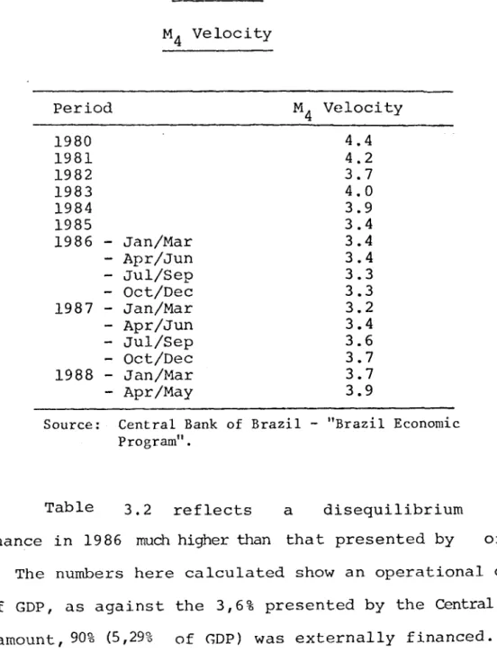
Begirming \Vi th Table 3.1, i t ean be noticed that the expan-sion of M4 was basieally ineampatible with the zero inflation target assumed

by arehitects of the Cruzado Plano 'lhe long n.m stability of M4 velocity (see Table 3.3) pointed out a high eorrelation between this aggregate and the naninal

national produet (1). In accordanee with this empirical observation, the rate

of exparsion of M4 should have been kept very close to zero, through the

con-trol of the consolidated Treasm:y' s and Central Bank' s liabili ties .

Table 3.3

M4 Ve10city

Period _{M4 Velocity}

1980 4.4

1981 4.2

1982 3.7

1983 4.0

1984 3.9

1985 3.4

1986 - Jan/Mar 3.4

- Apr/Jun 3.4

- Jul/Sep 3.3

- Oct/Dec 3.3

1987 - Jan/Mar 3.2

- Apr/Jun 3.4

- Jul/Sep 3.6

- Oct/Dec 3.7

1988 - Jan/Mar 3.7

- Apr/May 3.9

Source: Central Bank of Brazil - "Brazil Economic Program".

Table _{3.2 reflects a} disequi1ibrium in'

pub1ic finance in 1986 much higher than that presented by official

estimates. The nurnbers here calculated show an operational deficit

of 6,96% of GDP, as against the 3,6 % presented by the Central

From this amount, 90% (5,29% of GDP) was externa1ly financed.

Bank.

The

external financing is closeIy associated with the deterioration were of the cornrnercial balance which occurred in this year. ｾｲｴｳ＠

controlled and imports largely used to support the artificial pricc

(1) h · 11;gh corre lation is in par t d u e to the fact that mnst assets '.

'1'-Of _{included in} course t _{M4 ｾｳ＠ are indexed. However,} ... this does not imply non-contraL,b1. 1. ty.

.26.

controls. The contribution of external savings to minimize the

ex-ante excess demand translates into the sharp increase in the

current account deficit, which, in constante dolars of 1987, averaged

327 million dollars in 1984, 1985 and 1987, as agaist 4,6 billion

dollars in 1986.

The process of continued borrowing in foreign currency

by the government can also be observed in Table 3.2. Between 1984

and 1986, the part of the real deficit externally financed jumped,

as a percentage of GDP, from 0,44% in 1984, to 2,32%in 1985 and to

5,29% in 1986. In 1987 the process was reversed, with only 36% of

the governments budget deficit being externally financed (this

represented 1,57% of GDP) •

The evaluation of the real deficit is also useful,

since this is the concept ITDst oorrelated with ex-ante aqqreqate demand.

Indeed, when inflationary tax falls, the operational deficit rem:"lins

unchanged, but the real deficit increases. The same thing,

incidentally, happens with aggregate demand, since the avaiable real

income of the private sector (calculated with real.interest) increases.

In this way, the fact that the real deficit was bigger in 1986

than in any other year helps to explain the outburts of constlITption

which occured in this year. Besides the increase of real wages (1) ,

the fall of the real inflationary transfers from the private sector

to the Monetary Authori ties was one of the factors behind this facto The preceding discussion presents the reasons for

the failure of the Cruzado Plano FundamentaIs were not taken into

account as they should have been. Policy makers were too arnbiticus

(1) As shmm in Tab1e 4.3, average real wages increased around 19% between 1985 and 1986.

.27.

in establishing economic goals. In their own words, architects

of the Cruzado Plan stated it should "allow a growth like _Japan's

with an inflation rate like Switzerland's". Moreover, the Plan

should be able to reverse the effects of previous "unfair" economic

policies carried out in Brazil(l). Finally, it should serve as a

lesson to the Argentinians, who were regarded as facing an unnecessary

recession wi th their Austral Plan. The Cruzado Plan should dem:mstrate

that it was possible to tame inflation with no recession. At least

in one respect alI this presumption was useful: it could serve as

an appropriate mean of account to measure the proportionally huge

disaster.

The financiaI intermediation process in Brazil was

in many aspects influenced by the Cruzado Plan. The Brazilian banking

system, as shovln in chapter two, has been rewarded vlith considerable

real transfers from the non-banking system, due to the high rates

of inflation. Following the economic principIe by means of which

marginal costs should be increased up to the limit where they reach

marginal receipts, many banking agencies operated under circurnstances

that would not be profitable with zero inflation. The agencies

operated in remote geographical areas with excess employees, or

operated in largely competitive environrnents. In the first months

after the beginning of the Plan, when it was still believed (vlith

prices frozen) that zero inflation was a feasible target, analysts

expected the closing of some agencies and temporary difficulties

experienced by certa in banks. These developments really did take

place,but below the extent forescated. This because the governrnent

itself was also not prepared to live without an inflation taxo In

(1) This was said by the Labor Minister in a Conference held sometime after the starting of the Plano

l.n

são

Paulo

.28.

the very near future economic conditions would return to the previous

situation. Inflation would return to its old level(l)providingthe

banks and the government easy eccess to inflationary transfers and

to inflationary taxo

Just after introduction of the Cruzado Plan, the

stock exchanges experienced a sharp expansion. Exoectations about

future profits were most optimistic. Real interest

forescast to be kept very low, which supported

rates

the

were

initial

enthusiasm. At the same tilue, real estate prices jumped based on

the same reasons. Many micro-firms emerged with easy credit and

there was an outburst of aggregate demand. However when the failure

of the Plan became clear the situation completely reversed.

prices fell more rapidly than profits. The dollar price of

stock

a::-eal

estate also fell sharply. Many micro-firms becarre irlsolvent. Fortunately

for them, they were granted a partial debt amnesty by the new Consti tution.

This amnesty represents a heavy financiaI burden to the governrnent,

since most of the loans were provided by Banco do Brasil, and also

to private banks (the total amount of loans was 0,8% of GDP) •

With the sharp decline in inflation associated with

the Cruzado Plan, the deposits at "Caderneta de Poupança", the most

popular savings account in Brazil, declined at an alarming rate.

Since this indexed asset pays a constant real interest rate, despite

the rate of inflation, some analysts agreed that these withdrawals

constituted a clear evidence of "money illusion". One could find

many people at this time worried about the decline in monetary

correction credited to their savings accounts. Previously, 15%

monthly inflation generated fifteen Cruzados of deposits.Sare ｰＭｾｬ･＠

.29.

interpreted this as a real gain, rather than a simple replacement

of the purchasing power of the investment. It is interesting that

according to the econometric esti.ma tes presented in chapter two,

money illusion, if it ex1sted, was not significant on the whole. As

time goes on, those who spent their monetary correction revenues

realize that what they are really doing is depleting their accumulated

capital. Another reason, completely independent of money illusion,

can explain the large withdrawals from saving accounts. While the

real rate of interest was kept unchaged (6% per year on savings

deposits), the real interest paid by another asset, M_l, was increased

considerably with the decline in inflation. Consequently, there

was a portfolio reallocation based on the change of relative (real)

returns.

Wi th respect to the dollar black market, the situation

development much as in the introduction of the Austral Plan in

Argentina (June 16, 1985). Just before the Plan was launched, the

premium on the official market reached a peak, suddenly falling

after new measures were announced and understood by the population.

In Argentina, high (domestic) real interest rates perpetuated this

situation for some months. In Argentina, on some occasions, the

official doI lar quotation was even higher than the market quotation.

In Brazil, on the other hand, the black market premium soon began

to reflect an increasing suspicion concerning the success of the

Cruzado Plano Instead of increasing the real interest rate and

correcting the disequilibrium in public finances, nothing was

.30.

3) The Interdependence of Monetary_and Fiscal Policy

In the forty-one year period December 1946 to

December 1987, M

l increased by a factor of 23,582,766 times, wich means an average increase of 51,29% per year. An easy conclusion

to reach from these numbers is that the Brazilian monetary system

seems to have a natural propensity toward high growth of the money

supply. This can be attributed to a very simple reason: rroney issue

has always been under the control of the Executive. As noted from

Table 2.6, the use of an inflationary tax as a tool to generate

real current receipts has been an usual procedure, from Ol1e administration

to another. This kind of tax is particularly attractive to

policy--makers for two reasons: First, it is indirect, being paid by

those who hold cash balances during a given periodi Second, it is

an invisible tax which the average person cannot be aware of. Unlike

taxes generally levied by governments and collected in the form of

a physical transfer of money, the inflation tax does not generate a

payment or transfer of money.

Until 1964, there was no Central Bank in Brazil.

Monetary regulations were under the responsability of SUMOC

(Supe-rintendência da Moeda e do Crédito). Legal currency was issued by

the Federal Treasury, at the request of Banco do Brazil. The central

Bank of Brazil was created in 1965. The usual functions ascribed

to Central Banks were delegated to this institution: providing a

physical money supply, acting as a banker for banks, and as a fiscal

agent of the Treasury, and providing for the custody and register

of international reserves. While the new Central Bank assumed the

external appearance of other Central Banks, many things did not

.31.

former authority in matters relating to money and credit creation.

Money printing remained under control (now indirect) of the Minister

of Finance. Indeed, most relevant decisions regarding monetary and

foreign exchange matters have been taken, since 1965,by the ,National

Monetary Council (Conselho Nonetário Nacional, CMN) which is chaired

by the Minister of Finance. 'lhere is, even nowadays, no independence of the

Central ｅ｡ｮＮｾ＠ from the Executive. Directors of this institution can be

changed at any moment, at the discretion of the President of the

Republic. Their terms are not pre-established which makes them

subject to political pressures.

An important complication to Central Bank credit

control has been posed by the so called "movement account" (1) • This

facility allowed Banco do Brasil to withdraw monetary resources

at the Central Bank paying a nominal interest rate of 1% per year.

In effect, this made Banco do Brasil a second Central Bank, since

its active operations were not limited to its available resources,

but to the limits settled by the National Monetary Council. The

following illustration reflects how Banco do Brasil operations

actually generated a simultaneous increase in the stock of High

POvlered Money (the Monetary Base) .

Banro do Brasil Central Bank

Assets Liabilities Assets Liabilities

t:.

I.oans f.. M:>verrent Acrount

f.. r,t:M:>..lTent Account

(1) Nowadays (actually, as of March, 1986) ca11ed " supp 1y account" Suprimento) •

(Conta de

.32.

In effect, new loans provided by Banco do Brasil to the private

sector led to a drawing of funds from the movement account

consequently, to a expansion of the Monetary Base.

and,

Due to Banco do Brasil automatic access to monetary

resources provided by the Central Bank, the balance sheets of these

two institutions have been presented as consolidated,

designation "Monetary Authorities Balance Sheet".

under the

In theory, Banco do Brasil could use this rediscount

facility only up to the limits pre-determined by the CMN. Until

1979, excesses were penalized with heavy rediscount rates. From

1979 on these penalties were practically abolished. This situation

lasted until March, 1986, when policy-makers tried to eliminate the

role of Banco do Brasil as a Central Bank by extinguishing the

"movement Account" and creating the "supply account" ｾ＠ The difference

between the two is that, in the second case, the monetary

from Central Bank to Banco do Brasil should be subjected

transfers

to the

approval of the Secretary of the Treasury. Since the institutional

basis which determines the relationship between the

Treasury,

Banco

Central and Banco do Brasil were not effectively modified,the change

has been purely semantic. Invariably the Secretary of the Treasury

has not denied approval to most of Banco do Brasil expenditures.

This is because this institution (BB) is a strong political forcei

and because Banco do Brasil continued conducting operations (established

in prior agreements which were not modified) of interest of the ,Executive.

It should be noted these operations are largely disassociated from

normal commercial bank operations.

tvhile rnany things remained the same, in

(starting March 1986) Banco do Brasil is no longe r officialy

as a Monetary Autority. The demand deposits in Banco do

practice

classified

.33,.

which previous1y were counted as part of the stock of High powered

Money, are now considered to be part of commercia1 bank sight deJ.X>Sits,

and are not accounted in the Monetary Base. The Brazi1ian banking

mu1tip1ier and High powered Honey series must be ana1yzed with

care. Starting in March 1986 the 1atter decreased and the former

increased. The series organized under the new methodo1ogy were

published starting in December 1982. Although Banco do Brasil now

is treated as 3.ny other commercial bank, its function as a development

bank and as the government's bank remain pratically unchanged. An

indication that changes were purely semantic is given by the real

value of the transfers from the Central Bank to Banco do : Brasil.

They did not decrease after March 1986. In the twelve monthsperiód

before Harch, 1986, the transferences from Central Bank to Banco do

Bra-sil averaged, BCz$ 153,247(1). In the 23 months period later 02/88

(up to February, 1988) these transfers averaged BCz$ 201,075. 02/88

This is the best prove that the change of Banco do Brazil's status

was purely cosmetic.

The National Monetary Counci1 (CMN), the

decision-making organ related to monetary and foreign exchange po1icy, is

composed of five Hinisters of State, eight Chairmen of federal

financial institutions (including the Banco do Brasil and the

Central Bank), and by a fixed number of private advisors. As

previously mentioned, the Council is chaired by the Minister of

Finance. The CMN is responsible for the so-ca1led Monetary Budgct,

which refers to the several ceilings applied to aggregate monetary

expansion. Among the ceilings included in the Monetary Budget are

the maximum yearly expansion rate of the monetary base, means of

payment, and Banco do Brasil assets.

ｲＭＭＭＭＭＭＭＭＭＭＭＭＭＭＭＭＭＭＭＭＭｾｾＭＭＭＭＭＭＭ -- --- - --

--._--.34.

In addi tion to the Fiscal Budget, the evaluation of bréUilian fiscal policy is complicated by the existence of two additional

budgets: the IIMonetary Budget", which we have just referred to,

and the "State Enterprises Budget", which establishes ceilings for

state enterprises net financiaI borrowings. The co-existence of

the fiscal and monetary budget provided a way of transforming

Indced, many

large budget deficits into official surpluses.

operations of the Federal Government were included arrong the

assets and liabilities of the Mbnetary Authorities, often creating large current

defici ts, financed by increases in rroney suppl y. Since these defici ts , arising

from subsidized credits and transfers, were not included in the fiscal budget ｳｾ＠

mitted to the Congress, an official surplus could errerge.

One large government expense not included

fiscal budget was the payment of interest on the public

in the

deficit.

Since 1971, following the IILei Complementar número 1211

, the Central

Bank was allowed to issue Federal Government debt. It was a

counterpart of the many operations of the Federal Government arrried

out by the Monetary Authorities. Interest paid on the debt was

also under the responsibility of the Monetary Authorities, and was

not included in the fiscal budget.

Beginning in March 1986, many measures have been

introduced to simplify the complicated relations involving the

Federal Treasury, Central Bank and Banco do Brasil. The first we

have already described, that was to classify Banco do Brasil as a

commercial bank, rather than a Monetary Authority. Another group

of resolutions aimed at including in the fiscal budget alI current

expenditures of the federal governrnent carried out by the Central

.35.

represented by the Congress, the destination of taxes paid. Central

Bank power to issue debt in the name of the government was removed.

In addition the cost of the federal government debt service was

assigned to the Treasury Secretary(Secretaria do Tesouro). For this

purpose, the LBC (Letra do Banco Central, Central Bank short term

1iability) is being rep1aced by the LFT (Letra Financeira do

Tesou-rol as concerns open-market operations. An important

between LBC and LFT is that interest paid on LFT is to be

in the fiscal budget, since it is issued by the Treasury.

difference

included

The

Central Bank continues to act as a dealer for the Treasury. It

remains to be seen if this increased transparency wil1 resu1t in

increased budgetary efficiency by the Federal Government.

Another institutional change to accur as of 1989 is

the use of esclator clauses in the fiscal budget. Pratically, the

means of account in this budget will be the OTN, rather than the

cruzado. This procedure may be unavoidable, if one wants the

fiscal budget approved by the Congress to be representa tive of

actual expenses. Indeed, with a 15% - 20% monthly inflation, the

use of figures denominated in cruzados would ne subject to severe

changes. Monetary correction applied to federal government

securities would make the monthly budget expenses subject to large

upward revisions. On a cumulative basis these revisions in the

budget could inflate the budget deficit to a high percentage of

GDP. Evidence of the need to index the budget is given by the

recent(1986-87) past, when the figures initially determined for

the budget turned out to be totally inadequate re1ative to actual