www.biogeosciences.net/14/145/2017/ doi:10.5194/bg-14-145-2017
© Author(s) 2017. CC Attribution 3.0 License.
Transient dynamics of terrestrial carbon storage:
mathematical foundation and its applications
Yiqi Luo1,2, Zheng Shi1, Xingjie Lu3, Jianyang Xia4, Junyi Liang1, Jiang Jiang1, Ying Wang5, Matthew J. Smith6, Lifen Jiang1, Anders Ahlström7,8, Benito Chen9, Oleksandra Hararuk10, Alan Hastings11, Forrest Hoffman12, Belinda Medlyn13, Shuli Niu14, Martin Rasmussen15, Katherine Todd-Brown16, and Ying-Ping Wang3
1Department of Microbiology and Plant Biology, University of Oklahoma, Norman, Oklahoma, USA 2Department for Earth System Science, Tsinghua University, Beijing, China
3CSIRO Oceans and Atmosphere, Aspendale, Victoria, Australia
4School of Ecological and Environmental Sciences, East China Normal University, Shanghai, China 5Department of Mathematics, University of Oklahoma, Norman, Oklahoma, USA
6Computational Science Laboratory, Microsoft Research, Cambridge, UK
7Department of Earth System Science, Stanford University, Stanford, California, USA 8Department of Physical Geography and Ecosystem Science, Lund University, Lund, Sweden 9Department of Mathematics, University of Texas, Arlington, TX, USA
10Department of Natural Resource Sciences, McGill University, Montreal, Canada
11Department of Environmental Science and Policy, University of California, One Shields Avenue, Davis, CA 95616, USA 12Computational Earth Sciences Group, Oak Ridge National Laboratory, Oak Ridge, TN 37831, USA
13Hawkesbury Institute for the Environment, Western Sydney University, Penrith NSW 2751, Australia
14Institute of Geographic Sciences and Natural Resources Research, Chinese Academy of Sciences, Beijing, China 15Department of Mathematics, Imperial College, London, UK
16Biological Sciences Division, Pacific Northwest National Laboratory, Richland, Washington, USA
Correspondence to:Yiqi Luo ([email protected])
Received: 7 September 2016 – Published in Biogeosciences Discuss.: 16 September 2016 Revised: 9 December 2016 – Accepted: 12 December 2016 – Published: 12 January 2017
Abstract. Terrestrial ecosystems have absorbed roughly 30 % of anthropogenic CO2emissions over the past decades, but it is unclear whether this carbon (C) sink will endure into the future. Despite extensive modeling and experimental and observational studies, what fundamentally determines tran-sient dynamics of terrestrial C storage under global change is still not very clear. Here we develop a new framework for understanding transient dynamics of terrestrial C storage through mathematical analysis and numerical experiments. Our analysis indicates that the ultimate force driving ecosys-tem C storage change is the C storage capacity, which is jointly determined by ecosystem C input (e.g., net primary production, NPP) and residence time. Since both C input and residence time vary with time, the C storage capacity is time-dependent and acts as a moving attractor that actual C stor-age chases. The rate of change in C storstor-age is proportional to
the C storage potential, which is the difference between the current storage and the storage capacity. The C storage ca-pacity represents instantaneous responses of the land C cycle to external forcing, whereas the C storage potential repre-sents the internal capability of the land C cycle to influence the C change trajectory in the next time step. The influence happens through redistribution of net C pool changes in a network of pools with different residence times.
computation-ally feasible so that both C flux- and pool-related datasets can be used to better constrain model predictions of land C sequestration. Overall, this new mathematical framework of-fers new approaches to understanding, evaluating, diagnos-ing, and improving land C cycle models.
1 Introduction
Terrestrial ecosystems have been estimated to sequester ap-proximately 30 % of anthropogenic carbon (C) emissions in the past 3 decades (Canadell et al., 2007). Cumulatively, land ecosystems have sequestered more than 160 Gt C from 1750 to 2015 (Le Quéré et al., 2015). Without land C seques-tration, the atmospheric CO2 concentration would have in-creased by an additional 95 parts per million and resulted in more climate warming (Le Quéré et al., 2015). During 1 decade from 2005 to 2014, terrestrial ecosystems seques-trated 3±0.8 Gt C year−1 (Le Quéré et al., 2015), which
would cost 1 billion dollars if the equivalent amount of C was sequestrated using C capture and storage techniques (Smith et al., 2016). Thus, terrestrial ecosystems effectively mitigate global change through natural processes with minimal cost. Whether this terrestrial C sequestration will endure into the future, however, is not clear, making the mitigation of global change greatly uncertain. To predict future trajectories of C sequestration in the terrestrial ecosystems, it is essential to understand fundamental mechanisms that drive terrestrial C storage dynamics.
To predict future land C sequestration, the modeling com-munity has developed many C cycle models. According to a review by Manzoni and Porporato (2009), approximately 250 biogeochemical models have been published over a time span of 80 years to describe carbon and nitrogen miner-alization. The majority of those 250 models follow some mathematical formulations of ordinary differential equations. Moreover, many of those biogeochemical models incorpo-rate more and more processes in an attempt to simulate C cycle processes as realistically as possible (Oleson et al., 2013). As a consequence, terrestrial C cycle models have be-come increasingly complicated and less tractable. Almost all model intercomparison projects (MIPs), including those in-volved in the last three IPCC (Intergovernmental Panel on Climate Change) assessments, indicate that C cycle models have consistently projected widely spread trajectories of land C sinks and were also found to fit observations poorly (Todd-Brown et al., 2013; Luo et al., 2015). The lack of progress in uncertainty analysis urges us to understand the mathemati-cal foundation of those terrestrial C models so as to diagnose causes of model spreads and improve model predictive skills. Meanwhile, many countries have made great investments on various observational and experimental networks (or plat-forms) in hope of quantifying terrestrial C sequestration. For example, FLUXNET was established about 20 years ago
to quantify net ecosystem exchange (NEE) between the at-mosphere and biosphere (Baldocchi et al., 2001). Orbiting Carbon Observatory 2 (OCO-2) satellite was launched in 2014 to quantify carbon dioxide concentrations and distri-butions in the atmosphere at high spatiotemporal resolution to constrain land surface C sequestration (Hammerling et al., 2012). Networks of global change experiments have been de-signed to uncover processes that regulate ecosystem C se-questration (Rustad et al., 2001; Luo et al., 2011; Fraser et al., 2013; Borer et al., 2014). Massive data have been gener-ated from those observational systems and experimental net-works. They offer an unprecedented opportunity for advanc-ing our understandadvanc-ing of ecosystem processes and constrain-ing model prediction of ecosystem C sequestration. Indeed, many of those networks were initiated with the goal of im-proving our predictive capability. Yet the massive data have rarely been integrated into earth system models to constrain their predictions. It is a grand challenge in our era to develop innovative approaches to integration of big data into com-plex models so as to improve prediction of future ecosystem C sequestration.
From a system perspective, ecosystem C sequestration oc-curs only when the terrestrial C cycle is in a transient state, under which C influx into one ecosystem is larger than C ef-flux from the ecosystem. Olson (1963) is probably among the first to examine organic matter storage in forest floors from the system perspective. His analysis approximated steady-state storage of organic matter as a balance of litter pro-ducers and decomposers for different forest types. However, global change differentially influences various C cycle pro-cesses in ecosystems and results in transient dynamics of ter-restrial C storage (Luo and Weng, 2011). For example, rising atmospheric CO2 concentration primarily stimulates photo-synthetic C uptake, while climate warming likely enhances decomposition. When ecosystem C uptake increases in a uni-directional trend under elevated CO2, terrestrial C cycle is at disequilibrium, leading to net C storage. The net gained C is first distributed to different pools, each of which has a differ-ent turnover rate (or residence time) before C is evdiffer-entually released back to the atmosphere via respiration. Distribution of net C exchange to multiple pools with different residence times is an intrinsic property of an ecosystem to gradually equalize C efflux with influx (i.e., internal recovery force toward an attractor). In contrast, global change factors that cause changes in C input and decomposition are considered external forces that create disequilibrium through altering in-ternal C processes and pool sizes. The transient dynamics of terrestrial C cycle at disequilibrium are maintained by inter-actions of internal processes and external forces (Luo and Weng, 2011). Although the transient dynamics of terrestrial C storage have been conceptually discussed, we still lack a quantitative formulation to estimate transient C storage dy-namics in the terrestrial ecosystems.
ecosys-tems from a system perspective? We first reviewed the ma-jor processes that most models have incorporated to simulate terrestrial C sequestration. The review helps establish that terrestrial C cycle can be mathematically represented by a matrix equation. We also described the Terrestrial ECOsys-tem (TECO) model with its numerical experiments in sup-port of the mathematical analysis. We then presented results of mathematical analysis on determinants of the terrestrial C storage, direction and magnitude of C storage at a given time point, and numerical experiments to illustrate climate impacts on terrestrial C storage. We carefully discussed as-sumptions of those terrestrial C cycle models as represented by the matrix equation, the validity of this analysis, and two new concepts introduced in this study, which are C storage capacity and C storage potential. We also discussed the po-tential applications of this analysis to model uncertainty anal-ysis and data–model integration. Moreover, we proposed that the C storage potential be a targeted variable for research, trading, and government negotiation for C credit.
2 Methods
2.1 Mathematical representation of terrestrial C cycle This study was conducted mainly with mathematical analy-sis. We first established the basis of this analysis, which is that the majority of terrestrial C cycle models can be repre-sented by a matrix equation.
Hundreds of models have been developed to simulate ter-restrial C cycle (Manzoni and Porporato, 2009). All the mod-els have to simulate processes of photosynthetic C input, C allocation and transformation, and respiratory C loss. It is well understood that photosynthesis is a primary pathway of C flow into land ecosystems. Photosynthetic C input is usu-ally simulated according to carboxylation and electron trans-port rates (Farquhar et al., 1980). Ecosystem C influx varies with time and space mainly due to variations in leaf photo-synthetic capacity, leaf area index of canopy, and a suite of environmental factors such as temperature, radiation, and rel-ative humidity (or other water-related variables) (Potter et al., 1993; Sellers et al., 1996; Keenan et al., 2012; Walker et al., 2014; Parolari and Porporato, 2016).
Photosynthetically assimilated C is partly used for plant biomass growth and partly released back into the atmosphere through plant respiration. Plant biomass in leaves and fine roots usually lives for several months up to a few years be-fore death, while woody tissues may persist for hundreds of years in forests. Dead plant materials are transferred to lit-ter pools and decomposed by microorganisms to be partially released through heterotrophic respiration and partially sta-bilized to form soil organic matter (SOM). SOM can store C in the soil for hundreds or thousands of years before it is bro-ken down into CO2through microbial respiration (Luo and Zhou, 2006). This series of C cycle processes has been
repre-sented in most ecosystem models with multiple pools linked by C transfers among them (Jenkinson et al., 1987; Parton et al., 1987, 1988, 1993), including those embedded in Earth system models (Ciais et al., 2013).
The majority of the published 250 terrestrial C cycle mod-els use ordinary differential equations to describe C transfor-mation processes among multiple plant, litter, and soil pools (Manzoni and Porporato, 2009). Those ordinary differential equations can be summarized into a matrix formula (Luo et al., 2001, 2003, 2015, 2016; Luo and Weng, 2011; Sierra and Müller, 2015) as
X′(t )=Bu(t )−Aξ(t )KX(t )
X(t=0)=X0 , (1)
whereX′(t )is a vector of net C pool changes at timet,X(t ) is a vector of pool sizes, B is a vector of partitioning co-efficients from C input to each of the pools,u(t ) is C
in-put rate,Ais a matrix of transfer coefficients (or microbial C use efficiency) to quantify C movement along the path-ways,Kis a diagonal matrix of exit rates (mortality for plant pools and decomposition coefficients of litter and soil pools) from donor pools,ξ(t )is a diagonal matrix of environmental
scalars to represent responses of C cycle to changes in tem-perature, moisture, nutrients, litter quality, and soil texture, andX0 is a vector of initial values of pool sizes of X. In Eq. (1), all the off-diagonal elements of matrixA,aj i, are
negative to reverse the minus sign and indicate positive C influx to the receiving pools. The equation describes net C pool change,X′(t ), as a difference between C input,u(t ), distributed to different plant pools via partitioning coeffi-cients,B, and C loss through the C transformation matrix, Aξ(t )K, among individual pools,X(t ). Elements in vector
Band matricesAandKcould vary with many factors, such as vegetation types, soil texture, microbial attributes, and lit-ter chemistry. For example, vegetation succession may influ-ence elements in vectorBand matricesAandKin addition to C input,u(t ), and forcing that affects C dynamics through
environmental scalars,ξ(t ).
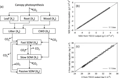
Figure 1.The Terrestrial ECOsystem (TECO) model and its outputs. Panel(a)is a schematic representation of C transfers among multiple pools in plant, litter, and soil in the TECO model. TECO has feedback loops of C among soil pools. CWD is coarse wood debris, SOM is soil organic matter. Panel(b)compares the original TECO model outputs with those from matrix equations for net ecosystem production (NEP is the sum of elements inX′(t )from Eq. 1). The perfect match between the TECO outputs and NEP from Eq. (1) is due to the fact that they are mathematically equivalent. Panel(c)compares the original TECO model outputs with those from matrix equations for ecosystem C storage (equal to the sum of elements inX(t )from Eq. 2). The C storage values calculated with Eq. (2) are close to a 1 : 1 line withr2=0.998 with the modeled values(c). The minor mismatch in estimated C storage between the matrix equation calculation and TECO outputs is due to numerical errors via inverse matrix operation with some small numbers.
2.2 TECO model, its physical emulator, and numerical experiments
We conducted numerical experiments to support mathe-matical analysis and thus help understand the characteris-tics of terrestrial C storage dynamics using the Terrestrial ECOsystem (TECO) model. TECO has five major compo-nents: canopy photosynthesis, soil water dynamics, plant growth, litter and soil carbon decomposition and transforma-tion, and nitrogen dynamics, as described in detail by Weng and Luo (2008) and Shi et al. (2016). Canopy photosynthesis is from a two-leaf (sunlit and shaded) model developed by Wang and Leuning (1998). This submodel simulates canopy conductance, photosynthesis, and partitioning of available energy. The model combines the leaf photosynthesis model developed by Farquhar et al. (1980) and a stomatal conduc-tance model (Harley et al., 1992). In the soil water dynamic submodel, soil is divided into 10 layers. The surface layer is 10 cm deep and the other nine layers are 20 cm deep. Soil water content (SWC) in each layer results from the mass bal-ance between water influx and efflux. The plant growth sub-model simulates C allocation and phenology. Allocation of C among three plant pools, which are leaf, fine root, and wood, depends on their growth rates (Fig. 1a). Phenology dynamics is related to leaf onset, which is triggered by growing degree days, and leaf senescence, which is determined by
tempera-ture and soil moistempera-ture. The C transformation submodel esti-mates carbon transfer from plants to two litter pools and three soil pools (Fig. 1a). The nitrogen (N) submodel is fully cou-pled with C processes with one additional mineral N pool. Nitrogen is absorbed by plants from mineral soil and then partitioned among leaf, woody tissues, and fine roots. Nitro-gen in plant detritus is transferred among different ecosystem pools (i.e., litter, coarse wood debris, and fast, slow, and pas-sive SOM) (Shi et al., 2016). The model is driven by climate data, which include air and soil temperature, vapor-pressure deficit, relative humidity, incident photosynthetically active radiation, and precipitation at hourly steps.
We first calibrated TECO with eddy flux data collected at Harvard Forest from 2006–2009. The calibrated model was spun up to the equilibrium state in preindustrial environmen-tal conditions by recycling a 10-year climate forcing (1850– 1859). Then the model was used to simulate C dynamics from 1850 to 2100 with the historical forcing scenario for 1850–2005 and RCP8.5 scenario for 2006–2100 as in the Community Land Model 4.5 (Oleson et al., 2013) in the grid cell where Harvard Forest is located.
parame-ter values in each of the C balance equations in the TECO model that correspond to elements in matricesA andKin Eq. (1). The time-dependent variables for u(t ), elements in
vectorB, and elements in matrixξ(t )in the physical
emula-tor were directly from outputs of the original TECO model. Then those parameter values and time-dependent variables were organized into matrices A,ξ(t ), andK; vectorsX(t ),
X0, andB; and variableu(t ). Note that values ofu(t ),B, andξ(t )could be different among different climate
scenar-ios. Those matrices, vectors, and variables were entered to matrix calculation to computeX′(t )using Eq. (1). The sum of elements in calculatedX′(t )is a 100 % match with simu-lated net ecosystem production (NEP) with the TECO model (Fig. 1b).
Once Eq. (1) was verified to exactly replicate TECO simu-lations, we used TECO to generate numerical experiments to support the mathematical analysis of the transient dynamics of terrestrial C storage. To analyze the seasonal patterns of C storage dynamics, we averaged 10 series of 3-year seasonal dynamics from 1851–1880. Then we used a 7-day moving window to further smooth the data.
3 Results
3.1 Determinants of C storage dynamics
The transient dynamics of terrestrial carbon storage are de-termined by two components: the C storage capacity and the C storage potential. The two components of C storage dy-namics can be mathematically derived by multiplying both sides of Eq. (1) by(Aξ(t )K)−1as
X(t )=(Aξ(t )K)−1Bu(t )−(Aξ(t )K)−1X′(t ). (2)
The first term on the right-hand side of Eq. (2) is the C stor-age capacity and the second term is the C storstor-age potential. Figure 2a shows time courses of C storage and its capacity over 1 year for the leaf pool of Harvard Forest.
In Eq. (2), we name the term(Aξ(t )K)−1the chasing time,
τch(t ), with a time unit used in exit rateK. The chasing time
is defined as
τch(t )=(Aξ(t )K)−1. (3)
τch(t )is a matrix of C residence times through the network
of individual pools, each with a different residence time and fractions of received C connected by pathways of C trans-fer. Analogous to the fundamental matrix measuring life ex-pectancies in demographic models (Caswell, 2000), the ma-trix, τch(t ), measures expected residence time of a C atom
in pooliwhen it has entered from poolj. We call this
ma-trix the fundamental mama-trix of chasing times to represent the timescale at which the net C pool change,X′(t ), is
re-distributed in the network. Meanwhile, the residence times of individual pools in the network,τN(t ), can be estimated
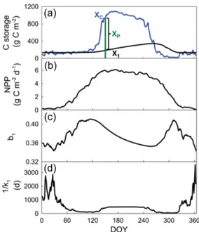
Figure 2.Seasonal cycles of C storage capacity and C storage dy-namics for the leaf pool (i.e., pool 1 as shown in Fig. 1). All the com-ponents are shown in panels(b–d)to calculatexc,1(t )=b1u(t )τ1 through multiplication, whereu(t )=NPP andτ1=1/k1for leaf.
by multiplying the fundamental matrix of chasing times,
(Aξ(t )K)−1, with a vector of partitioning coefficients,B, as
τN(t )=(Aξ(t )K)−1B. (4a)
Ecosystem residence time,τE(t ), is the sum of the residence
time of all individual pools in the network as
τE(t )=(1 1 . . . 1)τN(t ). (4b)
Thus, the C storage capacity can be defined by
Xc(t )=(Aξ(t )K)−1Bu(t ). (5a)
Alternatively, it can be estimated from C input,u(t ), and
res-idence time,τN(t ), as
Xc(t )=τN(t )u(t ). (5b)
The C storage potential at timet,Xp(t ), can be mathemat-ically described as
Xp(t )=(Aξ(t )K)−1X′(t ). (6a)
Or it can be estimated from net C pool change, X′(t ), and chasing time,τch(t )as
Xp(t )=τch(t )X′(t ). (6b)
Equation (6a) and (6b) suggest that the C storage potential represents redistribution of net C pool change,X′(t ), of
indi-vidual pools through a network of pools with different resi-dence times as connected by C transfers from one pool to the others through all the pathways. As time evolves, the net C pool change,X′(t ), is redistributed again and again through the network of pools. The network of redistribution of the next C pool change thus represents the potential of an ecosys-tem to store additional C when it is positive and lose C when it is negative. The C storage potential can also be estimated from the difference between the C storage capacity and the C storage itself at timetas
Xp(t )=Xc(t )−X(t ). (6c)
The C storage potential in the leaf pool, for example, is about zero in winter and early spring when the C storage capacity is very close to the storage itself (Fig. 2a). The C storage po-tential is positive when the capacity is larger than the storage itself from late spring to summer and early fall. As the stor-age capacity decreases to the point when the storstor-age equals the capacity on the 265th day of the year (DOY), the C stor-age potential is zero. After that day, the C storstor-age potential becomes negative.
Dynamics of ecosystem C storage,X(t ), can be
charac-terized by three parameters: C influx,u(t ), residence times,
τN(t ), and the C storage potential,Xp(t ), as
X(t )=τN(t )u(t )−Xp(t ). (7)
Equation (7) represents a three-dimensional (3-D) parameter space within which model simulation outputs can be placed to measure how and how much they diverge.
Note that sums of elements of vectorsX(t ),Xc(t ),Xp(t ),
andX′(t )correspond, respectively, to the whole ecosystem C stock, ecosystem C storage capacity, ecosystem C storage potential, and NEP. In this paper, we describe them wherever necessary rather than use a separate set of symbols to repre-sent those sums.
3.2 Direction and rate of C storage change at a given time
Like studying any moving object, quantifying dynamics of land C storage needs to determine both the direction and the rate of its change at a given time. To determine the direction and rate of C storage change, we rearranged Eq. (2) to be τchX′(t )=Xc(t )−X(t )=Xp(t ), (8a)
or rearranging Eq. (6a) leads to
X′(t )=Aξ(t )KXp(t ). (8b)
Since all the elements inτchare positive, the sign ofX′(t )is
the same as forXp(t ). That means thatX′(t )increases when Xc(t ) >X(t ), does not change whenXc(t )=X(t ), and
de-creases whenXc(t ) <X(t )at the ecosystem scale. Thus, the
C storage capacity, Xc(t ), is an attractor and hence
deter-mines the direction toward which the C storage,X(t ), chases
at any given time point. The rate of C storage change,X′(t ),
is proportional toXp(t )and is also regulated byτch. When we study C cycle dynamics, we are interested in understanding dynamics of not only a whole ecosystem but also individual pools. Equation (8a) can be used to derive equations to describe C storage change for anith pool as
n X
j=1
fijτixj′(t )= n X
j=1
fijτibju(t )−xi(t )=xp,i(t ), (9a)
wherenis the number of pools in a C cycle model, fij is
a fraction of C transferred from poolj toithrough all the
pathways,τimeasures residence times of individual pools in
isolation (in contrast toτN in the network),xj′ is the net C
change in thejth pool,bj is a partitioning coefficient of C
input to thejth pool,xi(t )is the C storage in theith pool, and
xp,i(t )is the C storage potential in theith pool. Equation (9a)
means that the C storage potential of each pool at time t, xp,i(t ), is the sum of all the individual net C pool change,
x′
j, multiplied by corresponding residence time spent in pool
icoming from poolj. Through rearrangement, Eq. (9a) can
be solved for each individual pool net C change as a function of C storage potential of all the pools as
xi′(t )=xc,i,u(t )−xc,i,p(t )−xi(t )
fiiτi
, (9b)
wherexc,i,u(t )= n P
j=1
fijτibju(t )for the maximal amount of
C that can transfer from C input to theith pool.xc,i,p(t )= n
P
j=1,j6=i
fijτixj′(t ) for the maximal amount of C that can
transfer from all the other pools to theith pool.fii=1 for
all the pools if there is no feedback of C among soil pools.
fii<1 when there are feedbacks of C among soil pools.
As plant pools get C only from photosynthetic C input,
u(t ), but not from other pools, the direction and rate of C
storage change in theith plant pool is determined by
xi′(t )= xc,i(t )−xi(t )
τi
=Xp,i(t )
τi
xc,i(t )=biu(t )τi
fori=1,2,3. (10)
The C storage capacity of plant pools equals the product of plant C input,u(t )(i.e., net primary production, NPP),
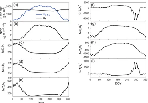
Figure 3.Seasonal cycles of the C storage capacity and C storage dynamics for the litter pool (i.e., pool 4 as shown in Fig. 1). All the
components are shown to calculatexc,4,u(t )= n P j=1
f4jτ4bju(t )in panels(b–e)andxc,4,p(t )= n P j=1,j6=4
f4jτ4x′j(t )in panels(f–i)for litter.
xc,4,u(t )is the maximal amount of C that can transfer from C input to the litter pool.xc,4,p(t )is the maximal amount of C that can transfer from all the other pools to the litter pool. This figure is to illustrate the network of pools through which C is distributed.
pool (Fig. 2b–d). Thus, the C storage capacities of the leaf, root, and wood pools are high in summer and low in win-ter. Plant C storage, xi(t ), still chases the storage
capac-ity,xc,i(t ), of its own pool at a rate that is proportional to
Xp,i(t ). For the leaf pool, the C storage, x1(t ), increases
when xc,1(t ) > x1(t )(or xp,1(t ) >0) from late spring until
early fall on the 265th day of the year (DOY) and then de-creases when xc,1(t ) < x1(t )(orxp,1(t ) <0) from 265 until
326 DOY during fall (Fig. 2a).
However, the direction of C storage change in litter and soil pools is no longer solely determined by the storage ca-pacity,xc,i(t ), of their own pools or at a rate that is
propor-tional toXp,i(t ). The C storage capacity of one litter or soil
pool has two components. One component,xc,i,u(t )is set by
the amount of plant C input,u(t ), going through all the
pos-sible pathways,fijbj, multiplied by residence time,τi, of its
own pool. The second component measures the C exchange of one litter or soil pool with other pools according to net C pool change,xj′(t ), through pathways,fij, j6=i, weighed
by residence time,τi, of its own pool. For example, C input
to the litter pool is a combination of C transfer from C in-put through the leaf, root, and wood pools (Fig. 3c, d, and e) and C transfer due to the net C pool changes in the leaf, root, and wood pools (Fig. 3f, g, and h). Thus, the first capacity component of the litter pool to store C is the sum of three products of NPP, C partitioning coefficient, and network res-idence time through the leaf, root, and wood pools, respec-tively (Fig. 3c, d, and e). The second capacity component is
the sum of the other three products of C transfer coefficient along all the possible pathways, network residence time, and net C pool changes in the leaf, root, and wood pools, respec-tively (Fig. 3f, g, and h). Thus, C storage in the ith pool, xi(t ), chases an attractor,
n X
j=1
fijbju (t )− n X
j=1,j6=i
fijτixj′(t ) !
τi,
for litter and soil pools (Fig. 4).
In summary, due to the network of C transfer, C storage in litter and soil pools does not chase the C storage capaci-ties of their own pools in a multiple C pool model (Fig. 4). The capacities for individual litter and soil pools measure the amount of C that is transferred from photosynthetic C in-put through plant pools to be stored in those pools. However, those litter and soil pools also exchange C with other pools according to transfer coefficients along pathways of C move-ment, multiplying net C pool change in those pools. Integra-tion of the C input and C exchanges together is still a moving attractor toward which individual pool C storage approaches (Fig. 4).
3.3 C storage dynamics under global change
Figure 4.Components of the C storage capacity for litter pool (i.e., pool 4 as shown in Fig. 1). Componentxc,4,u(t )is the C from C
in-put and componentxc,4,p(t )is the C moved from all the other pools to the litter pool. The sum of them is the attractor that determines the direction of C storage change in pool 4.
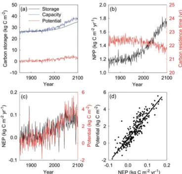
27 kg C m−2in 1850 to approximately 38 kg C m−2in 2100 with strong interannual variability (Fig. 5a). The increasing capacity results from a combination of a nearly 44 % increase in NPP with a∼2 % decrease in ecosystem residence times
(the sum of all elements in vectorτE(t ))during that period (Fig. 5b). The strong interannual variability in the modeled capacity is attributable to the variability in NPP and residence times, both of which directly respond to instantaneous vari-ations in environmental factors. In comparison, the ecosys-tem C storage (the sum of all elements in vectorX(t ))itself
gradually increases, lagging behind the capacity, with much dampened interannual variability (Fig. 5a). The dampened interannual variability is due to smoothing effects of pools with various residence times. In response to global change scenario RCP8.5, the ecosystem C storage potential (the sum of all elements in vectorXp(t ))in the Harvard Forest
ecosys-tem increases from zero at 1980 to 3.5 kg C m−2in 2100 with strong fluctuation over the years (Fig. 5a). Over seasons, the potential is high during the summer and low in winter, simi-lar to the seasonal cycle of the C storage capacity.
Since chasing time,τch, is a matrix and net C pool change, X′(t ), is a vector, Eq. (6a) or (6b) (i.e., the C storage
poten-tial) can not be analytically separated into the chasing time and net C pool change as the capacity can be into C input and residence time in Eq. (5a) or (5b) for traceability analy-sis. The relationships among the three quantities can be ex-plored using regression analysis. The ecosystem C storage potential fluctuates in a similar phase with NEP from 1850 to 2100 (Fig. 5c). Consequently, the C storage potential is well correlated with NEP at the whole ecosystem scale (Fig. 5d). The slope of the regression line is a statistical representa-tion of ecosystem chasing time. In this study, we find thatr2
of the relationship between the storage potential and NEP is 0.79. The regression slope is 28.1 years in comparison with the ecosystem residence time of approximately 22 years (Fig. 5b).
Figure 5.Transient dynamics of ecosystem C storage in response to global change in Harvard Forest. Panel(a)shows the time courses of the ecosystem C storage capacity, the ecosystem C storage po-tential, and ecosystem C storage (i.e., C stock) from 1850 to 2100. Panel(b)shows time courses of NPP(t) as C input and ecosystem residence times. Panel(c)shows correlated changes in ecosystem C storage potential and net ecosystem production (NEP). Panel(d) illustrates the regression between the C storage potential and NEP.
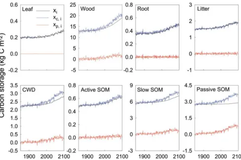
The capacity and storage of individual pools display sim-ilar long-term trends and interannual variability to those for the total ecosystem C storage dynamics (Fig. 6). Noticeably, the deviation of the C storage from the capacity, which is the C storage potential, is much larger for pools with long residence times than those with short residence times. For individual pools, the potential is nearly zero for those fast turnover pools and becomes very large for those pools with a long residence time (Fig. 6).
For individual plant pools, Eq. (10) describes the depen-dence of the C storage potential,xp,i(t ), on the pool-specific
residence time,τi, i=1, 2, and 3, and net C pool change of
their own pools,xi′(t ), i=1, 2, and 3. Thus, one value of
xp,i(t )corresponds exactly to one value ofxi′(t )at slope of
τi, leading to a correlation coefficient in Fig. 7 of 1.00 for
Figure 6.The C storage capacity (xc,i(t )), the C storage potential (xp,i(t )), and C storage (xi(t ))of individual pools. The potential is nearly
zero for those fast turnover pools with short residence times but very large for those pools with long residence times.
Figure 7.The C storage potential of individual pools (xp,i)as
in-fluenced by net C pool change of different pools (x′
i)in their
cor-responding rows. The correlation coefficients show the degree of influence of net C pool change in one pool on the C storage po-tential of the corresponding pool through the network of C transfer. The empty cells indicate no pathways of C transfer between those pools as indicated in Fig. 1.
4 Discussion
4.1 Assumptions of the C cycle models and validity of this analysis
This analysis is built upon Eq. (1), which represents the ma-jority of terrestrial C cycle models developed in the past
Second, those models all assume that multiple pools can adequately approximate transformation, decomposition, and stabilization of SOC in the real world (assumption 2). The classic SOC model, CENTURY, uses three conceptual pools, active, slow, and passive SOC, to represent SOC dynamics (Parton et al., 1987). Several models define pools that cor-respond to measurable SOC fractions to match experimen-tal observation with modeling analysis (Smith et al., 2002; Stewart et al., 2008). Carbon transformation in soil over time has also been described by a partial differential function of SOM quality (Bosatta and Ågren, 1991; Ågren and Bosatta, 1996). The latter quality model describes the external inputs of C with certain quality, C loss due to decomposition, and the internal transformations of the quality of soil organic mat-ter. It has been shown that multi-pool models can approx-imate the partial differential function or continuous quality model as the number of pools increases (Bolker et al., 1998; Sierra and Müller, 2015).
Assumption 3 is on partitioning coefficients of C input (i.e., elements in vector B) and C transformation among plant, litter, and soil pools (i.e., elements in the matrix Aξ(t )K). Some of the terrestrial C cycle models assume that
elements in vectorBand matricesAandKare constants. All the factors or processes that vary with time are represented in the diagonal matrixξ(t ). In the real world, C transformation
is influenced by environmental variables (e.g., temperature, moisture, oxygen, N, phosphorus, and acidity varying with soil profile, space, and time), litter quality (e.g., lignin, cel-lulose, N, or their relative content), organomineral proper-ties of SOC (e.g., complex chemical compounds, aggrega-tion, physiochemical binding and protecaggrega-tion, reactions with inorganic, reactive surfaces, and sorption), and microbial at-tributes (e.g., community structure, functionality, priming, acclimation, and other physiological adjustments) (Luo et al., 2016). It is not practical to incorporate all of those factors and processes into one model. Only a subset of them is explicitly expressed, while the majority is implicitly embedded in the C cycle models. Empirical studies have suggested that tem-perature, moisture, litter quality, and soil texture are primary factors that control C transformation processes of decompo-sition and stabilization (Burke et al., 1989; Adair et al., 2008; Zhang et al., 2008; Xu et al., 2012; Wang et al., 2013). Nitro-gen influences C cycle processes mainly through changes in photosynthetic C input, C partitioning, and decomposition. It is yet to be identified how other major factors and cesses, such as microbial activities and organomineral pro-tection, regulate C transformation.
Assumption 4 is that terrestrial C cycle models use dif-ferent response functions (i.e., difdif-ferent ξ(t ) in Eq. 1) to
represent C cycle responses to external variables. As tem-perature modifies almost all processes in the C cycle, dif-ferent formulations, including exponential, Arrhenius, and optimal response functions, have been used to describe C cycle responses to temperature changes in different mod-els (Lloyd and Taylor, 1994; Jones et al., 2005; Sierra and
Müller, 2015). Different response functions are used to con-nect C cycle processes with moisture, nutrient availability, soil clay content, litter quality, and other factors. Different formulations of response functions may result in substan-tially different model projections (Exbrayat et al., 2013) but are unlikely to change basic dynamics of the model behav-iors.
Assumption 5 is that disturbance events are represented in models in different ways (Grosse et al., 2011; West et al., 2011; Goetz et al., 2012; Hicke et al., 2012). Fire, ex-treme drought, insect outbreaks, land management, and land cover and land use change influence terrestrial C dynamics via (1) altering rate processes, for example, gross primary productivity (GPP), growth, tree mortality, or heterotrophic respiration; (2) modifying microclimatic environments; or (3) transferring C from one pool to another (e.g., from live to dead pools during storms or release to the atmosphere with fire) (Kloster et al., 2010; Thonicke et al., 2010; Luo and Weng, 2011; Prentice et al., 2011; Weng et al., 2012). Those disturbance influences can be represented in terrestrial C cycle models through changes in parameter values, envi-ronmental scalars, and/or discrete C transfers among pools of Eq. (1) (Luo and Weng, 2011). While Eq. (1) does not ex-plicitly incorporate disturbances for their influences on land C cycle, Weng et al. (2012) developed a disturbance regime model that combines Eq. (1) with frequency distributions of disturbance severity and intervals to quantify net biome ex-changes.
The sixth assumption that those models make is that the lateral C fluxes through erosion or local C drainage are neg-ligible so that Eq. (1) can approximate terrestrial C cycle over space. If soil erosion is substantial enough to be modeled with horizontal movement of C, a third dimension should be added in addition to two-dimensional transfers in classic models.
Our analysis on transient dynamics of terrestrial C cycle is valid unless some of the assumptions are violated. Assump-tion 1 on the first-order decay funcAssump-tion of decomposiAssump-tion ap-pears to be supported by thousands of datasets. It is a burden on microbiologists to identify empirical evidence to support the nonlinear microbial models. Assumption 2 may not affect the validity of our analysis no matter how C pools are divided in the ecosystems. Our analysis in this study is applicable no matter whether elements are time-varying or constant in vec-torBand matricesAandKas in assumption 3. Neither as-sumption 4 nor 5 would affect the analysis in this study. The environmental scalar,ξ(t ), as related to assumption 4 can be
4.2 Carbon storage capacity
One of the two components this analysis introduces to un-derstand transient dynamics of terrestrial C storage is the C storage capacity (Eq. 2). Olson (1963) is probably among the first who systematically analyzed C storage dynamics at the forest floor as functions of litter production and decompo-sition. He collected data of annual litter production and ap-proximately steady-state organic C storage at the forest floor, from which decomposition rates were estimated for a variety of ecosystems from Ghana in the tropics to alpine forests in California. Using the relationships among litter production, decomposition, and C storage, Olson (1963) explored sev-eral issues, such as decay without input, accumulation with continuous or discrete annual litter fall, and adjustments in production and decay parameters during forest succession. His analysis approximated the steady-state C storage as the C input times the inverse of decomposition (i.e., residence time). The steady-state C storage is also considered the max-imal amount of C that a forest can store.
This study is not only built upon Olson’s analysis but also expands it in at least two aspects. First, we similarly define the C storage capacity (i.e., Eq. 5a and 5b). Those equa-tions can be applied to a whole ecosystem with multiple C pools, while Olson’s analysis is for one C pool. Second, Ol-son (1963) treated the C input and decomposition rate as yearly constants at a given location even though they varied with locations. This study considers both C input and rate of decomposition being time dependent. A dynamical system with its input and parameters being time dependent math-ematically becomes a nonautonomous system (Kloeden and Rasmussen, 2011). As terrestrial C cycle under global change is transient, we need to treat it as a nonautonomous system to better understand the properties of transient dynamics. Ol-son (1963) approximated the nonautonomous system at the yearly timescale without global change so as to effectively understand properties of steady-state C storage at the forest floor. In comparison, Eq. (5a) and (5b) are not only more gen-eral but also essential for understanding transient dynamics of the terrestrial C cycle in response to global change.
Under the transient dynamics, the C storage capacity as defined by Eq. (5a) and (5b) still sets the maximal amount of C that one ecosystem can store at timet. This capacity
repre-sents instantaneous responses of ecosystem C cycle to exter-nal forcing via changes in both C input and residence time, and thus varies within 1 day, over seasons of a year, and inter-annually over longer timescales as forcings vary. The varia-tion of the C storage capacity can result from cyclic envi-ronmental changes (e.g., dial and seasonal changes), direc-tional global change (e.g., rising atmospheric CO2, nitrogen deposition, altered precipitation, and warming), disturbance events, disturbance regime shifts, and changing vegetation dynamics (Luo and Weng, 2011). Since the capacity sets the maximal amount of C storage (Fig. 2a), it is a moving attrac-tor toward which the current C sattrac-torage chases. When the
ca-pacity is larger than the C storage itself, C storage increases. Otherwise, the C storage decreases.
4.3 Carbon storage potential
The C storage potential represents the internal capability to equilibrate the current C storage with the capacity. Biogeo-chemically, the C storage potential represents redistribution of net C pool change, X′(t ), of individual pools through
a network of pools with different residence times as con-nected by C transfers from one pool to the others through all the pathways. The potential is conceptually equivalent to the magnitude of disequilibrium as discussed by Luo and Weng (2011).
Extensive studies have been done to quantify terrestrial C sequestration. The most commonly estimated quantities for C sequestration include net ecosystem exchange (NEE) and C stocks in ecosystems (i.e., plant biomass and SOC) and their changes (Baldocchi et al., 2001; Pan et al., 2013). This study, for the first time, offers the theoretical basis to estimate the terrestrial C storage potential in at least two approaches: (1) the product of chasing time and net C pool change with Eq. (6a) and (6b) and (2) the difference between the C stor-age capacity and the C storstor-age itself with Eq. (6c). Since the time-varying C storage capacity is fully defined by residence time and C input at any given time, C storage potential can be estimated from three quantities: C input, residence time, and C storage.
To effectively quantify the C storage potential in terrestrial ecosystems, we need various datasets from experimental and observatory studies to be first assimilated into models. For example, data from Harvard Forest were first used to con-strain the TECO model. The concon-strained model was used to explore changes in ecosystem C storage in response to global change scenario, RCP8.5. That scenario primarily stimulated NPP, which increased from 1.06 to 1.8 kg C m−2yr−1in the Harvard Forest (Fig. 5b). Although climate warming de-creased ecosystem C residence time in the Harvard Forest, the substantial increases in NPP resulted in increases in the C storage potential over time.
4.4 Novel approaches to model evaluation and improvement
com-putationally enable data assimilation to constrain complex models.
4.4.1 Physical emulators of land C cycle models We have developed matrix representations (i.e., physical emulators) of CABLE, LPJ-GUESS, CLM3.5, CLM4.0, CLM4.5, BEPS, and TECO (Xia et al., 2013; Hararuk et al., 2014; Ahlström et al., 2015; Chen et al., 2015). The emula-tors can exactly replicate simulations of C pools and fluxes with their original models when driven by a limited set of inputs from the full model (GPP, soil temperature, and soil moisture) (Fig. 1b and c). However, the physical emulators differ for different models since the elements of each matrix could be differently parameterized or formulized in different models. Also, different models usually have different pool-flux structures, leading to different non-zero elements in the Amatrix. Nonetheless, the physical emulators make complex models analytically clear, and therefore give us a way to un-derstand the effects of forcing, model structures, and param-eters on modeled ecosystem processes. They greatly simplify the task of understanding the dynamics of submodels and in-teractions between them. The emulators allow us to analyze model results in the 3-D parameter space and the traceability framework.
4.4.2 Parameter space of C cycle dynamics
Equation (7) indicates that transient dynamics of modeled C storage are determined by three parameters: C input, resi-dence time, and C storage potential. The 3-D parameter space offers one novel approach to uncertainty analysis of global C cycle models. As global land models incorporate more and more processes to simulate C cycle responses to global change, it becomes very difficult to understand or evaluate complex model behaviors. As such, differences in model pro-jections cannot be easily diagnosed and attributed to their sources (Chatfield, 1995; Friedlingstein et al., 2006; Luo et al., 2009). Equation (7) can help diagnose and evaluate plex models by placing all modeling results within one com-mon parameter space in spite of the fact that individual global models may have tens or hundreds of parameters to represent C cycle processes as affected by many abiotic and biotic fac-tors (Luo et al., 2016). The 3-D space can be used to measure how and how much the models diverge.
4.4.3 Traceability analysis
The two terms on the right side of Eq. (2) can be decomposed into traceable components (Xia et al., 2013) so as to identify sources of uncertainty in C cycle model projections. Model intercomparison projects (MIPs) all illustrate great spreads in projected land C sink dynamics across models (Todd-Brown et al., 2013; Tian et al., 2015). It has been extremely challeng-ing to attribute the uncertainty to sources. Placchalleng-ing simulation results of a variety of C cycle models within one common
pa-rameter space can measure how much the model differences are in a common metric (Eq. 7). The measured differences can be further attributed to sources in model structure, pa-rameter, and forcing fields with traceability analysis (Xia et al., 2013; Rafique et al., 2014; Ahlström et al., 2015; Chen et al., 2015). The traceability analysis can also be used to evalu-ate effectiveness of newly incorporevalu-ated modules into existing models, such as adding the N module on simulated C dynam-ics (Xia et al., 2013) and locate the origin of model ensemble uncertainties to external forcing vs. model structures and pa-rameters (Ahlström et al., 2015).
4.4.4 Constrained estimates of terrestrial C sequestration
Traditionally, global land C sink is indirectly estimated from airborne fraction of C emission and ocean uptake. Although many global land models have been developed to estimate land C sequestration, a variety of MIPs indicate that model predictions widely vary among them and do not fit obser-vations well (Schwalm et al., 2010; Luo et al., 2015; Tian et al., 2015). Moreover, the prevailing practices in the mod-eling community, unfortunately, may not lead to significant enhancements in our confidence on model predictions. For example, incorporating an increasing number of processes that influence the C cycle may represent the real-world phe-nomena more realistically but makes the models more com-plex and less tractable. MIPs have effectively revealed the ex-tent of the differences between model predictions (Schwalm et al., 2010; Keenan et al., 2012; De Kauwe et al., 2013) but provide limited insights into sources of model differ-ences (see Medlyn et al., 2015). The physical emulators make data assimilation computationally feasible for global C cycle models (Hararuk et al., 2014, 2015) and thus offer the pos-sibility to generate independent yet constrained estimates of global land C sequestration to be compared with the indirect estimate from the airborne fraction of C emission and ocean uptake. With the emulators, we can assimilate most of the C flux- and pool-related datasets into those models to better constrain global land C sink dynamics.
5 Concluding remarks
The C storage potential is the difference between the ca-pacity and the current C storage and thus measures the mag-nitude of disequilibrium in the terrestrial C cycle (Luo and Weng, 2011). The storage potential represents the internal capability (or recovery force) of the terrestrial C cycle to in-fluence the change in C storage in the next time step through redistribution of net C pool changes in a network of multi-ple pools with different residence times. The redistribution drives the current C storage towards the capacity and thus equilibrates C efflux with influx.
The two components of land C storage dynamics represent interactions of external forces (via changes in the capacity) and internal capability of the land C cycle (via changes in the C storage potential) to generate complex phenomena of C cy-cle dynamics, such as fluctuations, directional changes, and tipping points, in the terrestrial ecosystems. From a system perspective, these complex phenomena can not be generated by relatively simple internal processes but are mostly caused by multiple environmental forcing variables interacting with internal processes over different temporal and spatial scales, as explained by Luo and Weng (2011) and Luo et al. (2015). Note that while those internal processes can be mathemati-cally represented with a relatively simple formula, their eco-logical and bioeco-logical underpinnings can be very complex.
The theoretical framework developed in this study has the potential to revolutionize model evaluation. Our analysis in-dicates that the matrix equation as in Eqs. (1) and (2) can adequately emulate most of the land C cycle models. In-deed, we have developed physical emulators of several global land C cycle models. In addition, predictions of C dynamics with complex land models can be placed in a 3-D parameter space as a common metric to measure how much model pre-dictions are different. The latter can be traced to its source components by decomposing model predictions to a hierar-chy of traceable components. Moreover, the physical emula-tors make it computationally possible to assimilate multiple sources of data to constrain predictions of complex models.
The theoretical framework we developed in this study can explain dynamics of C storage in response to cyclic sea-sonal change in external forcings (e.g., Figs. 2 and 3), cli-mate change, and rising atmospheric CO2 well (Fig. 5). It can also explain responses of ecosystem C storage to dis-turbances and other global change factors, such as nitrogen deposition, land use changes, and altered precipitation. The theoretical framework is simple and straightforward but able to characterize the direction and rate of C storage change, which are arguably among the most critical issues for quan-tifying terrestrial C sequestration. Future research should ex-plicitly incorporate stochastic disturbance regime shifts (e.g., Weng et al., 2012) and vegetation dynamics (Moorcroft et al., 2001; Purves and Pacala, 2008; Fisher et al., 2010; Weng et al., 2015) into this theoretical framework to explore their the-oretical issues related to biogeochemistry.
6 Code availability
Computer code of the TECO model and its physical emulator are available at Yiqi Luo’s website (EcoLab, 2017).
Acknowledgements. This work was partially done through the working group, Nonautonomous Systems and Terrestrial Carbon Cycle, at the National Institute for Mathematical and Biological Synthesis, an institute sponsored by the National Science Foundation, the US Department of Homeland Security, and the US Department of Agriculture through NSF award no. EF-0832858, with additional support from the University of Ten-nessee, Knoxville. Research in Yiqi Luo EcoLab was financially supported by US Department of Energy grants DE-SC0008270, DE-SC0014085, and US National Science Foundation (NSF) grants EF 1137293 and OIA-1301789.
Edited by: A. V. Eliseev
Reviewed by: two anonymous referees
References
Adair, E. C., Parton, W. J., Del Grosso, S. J., Silver, W. L., Harmon, M. E., Hall, S. A., Burke, I. C., and Hart, S. C.: Simple three-pool model accurately describes patterns of long-term litter decompo-sition in diverse climates, Glob. Change Biol., 14, 2636–2660, 2008.
Ågren, G. I. and Bosatta, E.: Quality: A bridge between theory and experiment in soil organic matter studies, Oikos, 76, 522–528, 1996.
Ahlström, A., Xia, J. Y., Arneth, A., Luo, Y. Q., and Smith, B.: Importance of vegetation dynamics for future terrestrial car-bon cycling, Environ. Res. Lett., 10, 054019 doi:10.1088/1748-9326/10/5/054019, 2015.
Allison, S. D., Wallenstein, M. D., and Bradford, M. A.: Soil-carbon response to warming dependent on microbial physiology, Nat. Geosci., 3, 336–340, 2010.
Baldocchi, D., Falge, E., Gu, L. H., Olson, R., Hollinger, D., Running, S., Anthoni, P., Bernhofer, C., Davis, K., Evans, R., Fuentes, J., Goldstein, A., Katul, G., Law, B., Lee, X. H., Malhi, Y., Meyers, T., Munger, W., Oechel, W., Paw U, K. T., Pilegaard, K., Schmid, H. P., Valentini, R., Verma, S., Vesala, T., Wilson, K., and Wofsy, S.: FLUXNET: A new tool to study the tempo-ral and spatial variability of ecosystem-scale carbon dioxide, wa-ter vapor, and energy flux densities, B. Am. Meteorol. Soc., 82, 2415–2434, 2001.
Bolker, B. M., Pacala, S. W., and Parton, W. J.: Linear analysis of soil decomposition: Insights from the century model, Ecol. Appl., 8, 425–439, 1998.
Borer, E. T., Harpole, W. S., Adler, P. B., Lind, E. M., Orrock, J. L., Seabloom, E. W., and Smith, M. D.: Finding generality in ecology: a model for globally distributed experiments, Methods in Ecology and Evolution, 5, 65–73, 2014.
Burke, I. C., Yonker, C. M., Parton, W. J., Cole, C. V., Flach, K., and Schimel, D. S.: Texture, Climate, and Cultivation Effects on Soil Organic-Matter Content in US Grassland Soils, Soil Sci. Soc. Am. J., 53, 800–805, 1989.
Canadell, J. G., Le Quéré, C., Raupach, M. R., Field, C. B., Buiten-huis, E. T., Ciais, P., Conway, T. J., Gillett, N. P., Houghton, R. A., and Marland, G.: Contributions to accelerating atmospheric CO2growth from economic activity, carbon intensity, and effi-ciency of natural sinks, P. Natl. Acad. Sci. USA, 104, 18866– 18870, 2007.
Caswell, H.: Prospective and retrospective perturbation analyses: their roles in conservation biology, Ecology, 81, 619–627, 2000. Chatfield, C.: Model uncertainty, data mining and
statistical-inference, J. Roy. Stat. Soc. A Sta., 158, 419–466, 1995. Chen, Y., Xia, J., Sun, Z., Li, J., Luo, Y., Gang, C., and Wang, Z.:
The role of residence time in diagnostic models of global car-bon storage capacity: model decomposition based on a traceable scheme, Scientific reports, 5, 16155, doi:10.1038/srep16155, 2015.
Ciais, P., Gasser, T., Paris, J. D., Caldeira, K., Raupach, M. R., Canadell, J. G., Patwardhan, A., Friedlingstein, P., Piao, S. L., and Gitz, V.: Attributing the increase in atmospheric CO2 to emitters and absorbers, Nature Climate Change, 3, 926–930, 2013.
De Kauwe, M. G., Medlyn, B. E., Zaehle, S., Walker, A. P., Dietze, M. C., Hickler, T., Jain, A. K., Luo, Y., Parton, W. J., Prentice, I. C., Smith, B., Thornton, P. E., Wang, S., Wang, Y.-P., Wårlind, D., Weng, E., Crous, K. Y., Ellsworth, D. S., Hanson, P. J., Seok Kim, H., Warren, J. M., Oren, R., and Norby, R. J.: Forest wa-ter use and wawa-ter use efficiency at elevated CO2: a model-data intercomparison at two contrasting temperate forest FACE sites, Glob. Change Biol., 19, 1759–1779, 2013.
EcoLab: available at: http://ecolab.ou.edu/download/ TECOEmulator.php, last access: 6 January 2017.
English, B. P., Min, W., Van Oijen, A. M., Lee, K. T., Luo, G., Sun, H., Cherayil, B. J., Kou, S., and Xie, X. S.: Ever-fluctuating single enzyme molecules: Michaelis-Menten equation revisited, Nature Chem. Biol., 2, 87–94, 2006.
Exbrayat, J.-F., Pitman, A. J., Zhang, Q., Abramowitz, G., and Wang, Y.-P.: Examining soil carbon uncertainty in a global model: response of microbial decomposition to temperature, moisture and nutrient limitation, Biogeosciences, 10, 7095– 7108, doi:10.5194/bg-10-7095-2013, 2013.
Farquhar, G., von Caemmerer, S. V., and Berry, J.: A biochemi-cal model of photosynthetic CO2 assimilation in leaves of C3 species, Planta, 149, 78–90, 1980.
Fisher, R., McDowell, N., Purves, D., Moorcroft, P., Sitch, S., Cox, P., Huntingford, C., Meir, P., and Ian Woodward, F.: Assessing uncertainties in a second generation dynamic vegetation model caused by ecological scale limitations, New Phytol., 187, 666– 681, 2010.
Fraser, L. H., Henry, H. A., Carlyle, C. N., White, S. R., Beierkuhn-lein, C., Cahill, J. F., Casper, B. B., Cleland, E., Collins, S. L., and Dukes, J. S.: Coordinated distributed experiments: an emerging tool for testing global hypotheses in ecology and environmental science, Front. Ecol. Environ., 11, 147–155, 2013.
Friedlingstein, P., Cox, P., Betts, R., Bopp, L., Von Bloh, W., Brovkin, V., Cadule, P., Doney, S., Eby, M., Fung, I., Bala, G., John, J., Jones, C., Joos, F., Kato, T., Kawamiya, M., Knorr, W.,
Lindsay, K., Matthews, H. D., Raddatz, T., Rayner, P., Reick, C., Roeckner, E., Schnitzler, K. G., Schnur, R., Strassmann, K., Weaver, A. J., Yoshikawa, C., and Zeng, N.: Climate-carbon cy-cle feedback analysis: Results from the (CMIP)-M-4 model in-tercomparison, J. Climate, 19, 3337–3353, 2006.
Goetz, S. J., Bond-Lamberty, B., Law, B. E., Hicke, J. A., Huang, C., Houghton, R. A., McNulty, S., O’Halloran, T., Harmon, M., Meddens, A. J. H., Pfeifer, E. M., Mildrexler, D., and Kasis-chke, E. S.: Observations and assessment of forest carbon dy-namics following disturbance in North America, J. Geophys. Res.-Biogeo., 117, G02022, doi:10.1029/2011JG001733, 2012. Goldbeter, A.: Oscillatory enzyme reactions and Michaelis–Menten
kinetics, FEBS letters, 587, 2778–2784, 2013.
Grosse, G., Harden, J., Turetsky, M., McGuire, A. D., Camill, P., Tarnocai, C., Frolking, S., Schuur, E. A. G., Jorgenson, T., Marchenko, S., Romanovsky, V., Wickland, K. P., French, N., Waldrop, M., Bourgeau-Chavez, L., and Striegl, R. G.: Vul-nerability of high-latitude soil organic carbon in North Amer-ica to disturbance, J. Geophys. Res.-Biogeo., 116, G00K06, doi:10.1029/2010JG001507, 2011.
Hammerling, D. M., Michalak, A. M., and Kawa, S. R.: Mapping of CO2 at high spatiotemporal resolution using satellite obser-vations: Global distributions from OCO-2, J. Geophys. Res.-Atmos., 117, D06306, doi:10.1029/2011JD017015, 2012. Hararuk, O., Xia, J. Y., and Luo, Y. Q.: Evaluation and improvement
of a global land model against soil carbon data using a Bayesian Markov chain Monte Carlo method, J. Geophys. Res.-Biogeo., 119, 403–417, 2014.
Hararuk, O., Smith, M. J., and Luo, Y. Q.: Microbial models with data-driven parameters predict stronger soil carbon responses to climate change, Glob. Change Biol., 21, 2439–2453, 2015. Harley, P., Thomas, R., Reynolds, J., and Strain, B.: Modelling
pho-tosynthesis of cotton grown in elevated CO2, Plant Cell Environ., 15, 271–282, 1992.
Hicke, J. A., Allen, C. D., Desai, A. R., Dietze, M. C., Hall, R. J., Hogg, E. H., Kashian, D. M., Moore, D., Raffa, K. F., Sturrock, R. N., and Vogelmann, J.: Effects of biotic disturbances on forest carbon cycling in the United States and Canada, Glob. Change Biol., 18, 7–34, 2012.
Jenkinson, D., Hart, P., Rayner, J., and Parry, L.: Modelling the turnover of organic matter in long-term experiments at Rotham-sted, US9022414, available at: http://agris.fao.org/aos/records/ US9022414 (last access: 6 January 2017), 1987.
Jones, C., McConnell, C., Coleman, K., Cox, P., Falloon, P., Jenkin-son, D., and PowlJenkin-son, D.: Global climate change and soil carbon stocks; predictions from two contrasting models for the turnover of organic carbon in soil, Glob. Change Biol., 11, 154–166, 2005. Keenan, T. F., Baker, I., Barr, A., Ciais, P., Davis, K., Dietze, M., Dragoni, D., Gough, C. M., Grant, R., Hollinger, D., Hufkens, K., Poulter, B., McCaughey, H., Raczka, B., Ryu, Y., Schaefer, K., Tian, H., Verbeeck, H., Zhao, M., and Richardson, A. D.: Terrestrial biosphere model performance for inter-annual vari-ability of land-atmosphere CO2exchange, Glob. Change Biol., 18, 1971–1987, 2012.
Kloeden, P. E. and Rasmussen, M.: Nonautonomous dynamical sys-tems, Am. Math. Soc., Mathematical Surveys and Monographs, 176, 264 pp., 2011.
Ole-son, K. W., and Lawrence, D. M.: Fire dynamics during the 20th century simulated by the Community Land Model, Biogeo-sciences, 7, 1877–1902, doi:10.5194/bg-7-1877-2010, 2010. Le Quéré, C., Moriarty, R., Andrew, R. M., Canadell, J. G., Sitch, S.,
Korsbakken, J. I., Friedlingstein, P., Peters, G. P., Andres, R. J., Boden, T. A., Houghton, R. A., House, J. I., Keeling, R. F., Tans, P., Arneth, A., Bakker, D. C. E., Barbero, L., Bopp, L., Chang, J., Chevallier, F., Chini, L. P., Ciais, P., Fader, M., Feely, R. A., Gkritzalis, T., Harris, I., Hauck, J., Ilyina, T., Jain, A. K., Kato, E., Kitidis, V., Klein Goldewijk, K., Koven, C., Landschützer, P., Lauvset, S. K., Lefèvre, N., Lenton, A., Lima, I. D., Metzl, N., Millero, F., Munro, D. R., Murata, A., Nabel, J. E. M. S., Nakaoka, S., Nojiri, Y., O’Brien, K., Olsen, A., Ono, T., Pérez, F. F., Pfeil, B., Pierrot, D., Poulter, B., Rehder, G., Rödenbeck, C., Saito, S., Schuster, U., Schwinger, J., Séférian, R., Steinhoff, T., Stocker, B. D., Sutton, A. J., Takahashi, T., Tilbrook, B., van der Laan-Luijkx, I. T., van der Werf, G. R., van Heuven, S., Van-demark, D., Viovy, N., Wiltshire, A., Zaehle, S., and Zeng, N.: Global Carbon Budget 2015, Earth Syst. Sci. Data, 7, 349–396, doi:10.5194/essd-7-349-2015, 2015.
Li, J. W., Luo, Y. Q., Natali, S., Schuur, E. A. G., Xia, J. Y., Kowal-czyk, E., and Wang, Y. P.: Modeling permafrost thaw and ecosys-tem carbon cycle under annual and seasonal warming at an Arctic tundra site in Alaska, J. Geophys. Res.-Biogeo., 119, 1129–1146, 2014.
Lloyd, J. and Taylor, J. A.: On the Temperature-Dependence of Soil Respiration, Funct. Ecol., 8, 315–323, 1994.
Luo, Y. and Zhou, X.: Soil respiration and the environment, Aca-demic Press, Burlington, MA, USA, 2006.
Luo, Y., Weng, E., Wu, X., Gao, C., Zhou, X., and Zhang, L.: Pa-rameter identifiability, constraint, and equifinality in data assim-ilation with ecosystem models, Ecol. Appl., 19, 571–574, 2009. Luo, Y., Ahlström, A., Allison, S. D., Batjes, N. H., Brovkin, V.,
Carvalhais, N., Chappell, A., Ciais, P., Davidson, E. A., Finzi, A., Georgiou, K., Guenet, B., Hararuk, O., Harden, J. W., He, Y., Hopkins, F., Jiang, L., Koven, C., Jackson, R. B., Jones, C. D., Lara, M. J., Liang, J., McGuire, A. D., Parton, W., Peng, C., Randerson, J. T., Salazar, A., Sierra, C. A., Smith, M. J., Tian, H., Todd-Brown, K. E. O., Torn, M., van Groenigen, K. J., Wang, Y. P., West, T. O., Wei, Y., Wieder, W. R., Xia, J., Xu, X., Xu, X., and Zhou, T.: Toward more realistic projections of soil carbon dynamics by Earth system models, Global Biogeochem. Cy., 30, 40–56, 2016.
Luo, Y. Q. and Weng, E. S.: Dynamic disequilibrium of the terres-trial carbon cycle under global change, Trend. Ecol. Evol., 26, 96–104, 2011.
Luo, Y. Q., Wu, L., Andrews, J. A., White, L., Matamala, R., Schafer, K. V. R., and Schlesinger, W. H.: Elevated CO2 differ-entiates ecosystem carbon processes: Deconvolution analysis of Duke Forest FACE data, Ecol. Monogr., 71, 357–376, 2001. Luo, Y. Q., White, L. W., Canadell, J. G., DeLucia, E. H., Ellsworth,
D. S., Finzi, A. C., Lichter, J., and Schlesinger, W. H.: Sustain-ability of terrestrial carbon sequestration: A case study in Duke Forest with inversion approach, Global Biogeochem. Cy., 17, 1021, doi:10.1029/2002GB001923, 2003.
Luo, Y. Q., Ogle, K., Tucker, C., Fei, S. F., Gao, C., LaDeau, S., Clark, J. S., and Schimel, D. S.: Ecological forecasting and data assimilation in a data-rich era, Ecol. Appl., 21, 1429–1442, 2011.
Luo, Y. Q., Keenan, T. F., and Smith, M.: Predictability of the ter-restrial carbon cycle, Glob. Change Biol., 21, 1737–1751, 2015. Manzoni, S. and Porporato, A.: Soil carbon and nitrogen mineral-ization: theory and models across scales, Soil Biol. Biochem., 41, 1355–1379, 2009.
Matamala, R., Jastrow, J. D., Miller, R. M., and Garten, C. T.: Tem-poral changes in C and N stocks of restored prairie: Implications for C sequestration strategies, Ecol. Appl., 18, 1470–1488, 2008. Medlyn, B. E., Zaehle, S., De Kauwe, M. G., Walker, A. P., Dietze, M. C., Hanson, P. J., Hickler, T., Jain, A. K., Luo, Y., Parton, W., Prentice, I. C., Thornton, P. E., Wang, S., Wang, Y.-P., Weng, E., Iversen, C. M., McCarthy, H. R., Warren, J. M., Oren, R., and Norby, R. J.: Using ecosystem experiments to improve vegetation models, Nature Climate Change, 5, 528–534, 2015.
Moorcroft, P., Hurtt, G., and Pacala, S. W.: A method for scaling vegetation dynamics: the ecosystem demography model (ED), Ecol. Monogr., 71, 557–586, 2001.
Oleson, K., Lawrence, D., Bonan, G., Drewniak, B., Huang, M., Koven, C., Levis, S., Li, F., Riley, W., and Subin, Z.: Technical description of version 4.5 of the Community Land Model (CLM), National Center for Atmospheric Research, Boulder, Colorado, 2013.
Olson, J. S.: Energy storage and the balance of producers and de-composers in ecological systems, Ecology, 44, 322–331, 1963. Pan, Y., Birdsey, R. A., Phillips, O. L., and Jackson, R. B.: The
structure, distribution, and biomass of the world’s forests, Annu. Rev. Ecol. Evol. S., 44, 593–622, 2013.
Parolari, A. and Porporato, A.: Forest soil carbon and nitrogen cycles under biomass harvest: stability, transient response, and feedback, Ecol. Model., 329, 64–76, 2016
Parton, W. J., Schimel, D. S., Cole, C. V., and Ojima, D. S.: Anal-ysis of Factors Controlling Soil Organic-Matter Levels in Great-Plains Grasslands, Soil Sci. Soc. Am. J., 51, 1173–1179, 1987. Parton, W. J., Stewart, J. W. B., and Cole, C. V.: Dynamics of C,
N, P and S in Grassland Soils – a Model, Biogeochemistry, 5, 109–131, 1988.
Parton, W. J., Scurlock, J. M. O., Ojima, D. S., Gilmanov, T. G., Sc-holes, R. J., Schimel, D. S., Kirchner, T., Menaut, J. C., Seastedt, T., Moya, E. G., Kamnalrut, A., and Kinyamario, J. I.: Observa-tions and Modeling of Biomass and Soil Organic-Matter Dynam-ics for the Grassland Biome Worldwide, Global Biogeochem. Cy., 7, 785–809, 1993.
Potter, C. S., Randerson, J. T., Field, C. B., Matson, P. A., Vitousek, P. M., Mooney, H. A., and Klooster, S. A.: Terrestrial Ecosys-tem Production: a Process Model-Based on Global Satellite and Surface Data, Global Biogeochem. Cy., 7, 811–841, 1993. Prentice, I. C., Kelley, D. I., Foster, P. N., Friedlingstein, P.,
Har-rison, S. P., and Bartlein, P. J.: Modeling fire and the terres-trial carbon balance, Global Biogeochem. Cy., 25, GB3005, doi:10.1029/2010GB003906, 2011.
Purves, D. and Pacala, S.: Predictive models of forest dynamics, Science, 320, 1452–1453, 2008.
Rafique, R., Xia, J., Hararuk, O., and Luo, Y.: Structural analysis of three global land models on carbon cycle simulations using a traceability framework, Biogeosciences Discuss., 11, 9979– 10014, doi:10.5194/bgd-11-9979-2014, 2014.