A global water scarcity assessment under shared socio-economic pathways – Part 2: Water availability and scarcity

(1)

HESSD

9, 13933–13994, 2012

A global water scarcity assessment

– Part 2

N. Hanasaki et al.

Title Page Abstract Introduction Conclusions References

Tables Figures

◭ ◮

Back Close

Full Screen / Esc

Printer-friendly Version Interactive Discussion

Discussion

P

a

per

|

Dis

cussion

P

a

per

|

Discussion

P

a

per

|

Discussio

n

P

a

per

|

Hydrol. Earth Syst. Sci. Discuss., 9, 13933–13994, 2012 www.hydrol-earth-syst-sci-discuss.net/9/13933/2012/ doi:10.5194/hessd-9-13933-2012

Hydrology and Earth System Sciences Discussions

This discussion paper is/has been under review for the journal Hydrology and Earth System Sciences (HESS). Please refer to the corresponding final paper in HESS if available.

A global water scarcity assessment under

shared socio-economic pathways – Part

2: Water availability and scarcity

N. Hanasaki1, S. Fujimori1, T. Yamamoto2, S. Yoshikawa3, Y. Masaki1, Y. Hijioka1, M. Kainuma1, Y. Kanamori1, T. Masui1, K. Takahashi1, and S. Kanae3

1

National Institute for Environmental Studies, Tsukuba, Japan 2

Nagaoka National College of Technology, Nagaoka, Japan 3

Tokyo Institute of Technology, Tokyo, Japan

Received: 28 November 2012 – Accepted: 10 December 2012 – Published: 18 December 2012

Correspondence to: N. Hanasaki ([email protected])

(2)

HESSD

9, 13933–13994, 2012

– Part 2

N. Hanasaki et al.

Tables Figures

◭ ◮

Back Close

Full Screen / Esc

Discussion

P

a

per

|

Dis

cussion

P

a

per

|

Discussion

P

a

per

|

Discussio

n

P

a

per

|

Abstract

A global water scarcity assessment for the 21st century was conducted under the latest socio-economic scenario for global change studies, namely Shared Socio-economic Pathways (SSPs). SSPs depict five global situations with substantially different socio-economic conditions. In the accompanying paper, a water use scenario compatible with

5

the SSPs was developed. This scenario considers not only quantitative socio-economic factors such as population and electricity production but also qualitative ones such as the degree of technological change and overall environmental consciousness. In this paper, water availability and water scarcity were assessed using a global hydrologi-cal model hydrologi-called H08. H08 simulates both the natural water cycle and major human

10

activities such as water withdrawal and reservoir operation. It simulates water avail-ability and use at daily time intervals at a spatial resolution of 0.5◦×0.5◦. A series of global hydrological simulations were conducted under the SSPs, taking into account di_fferent climate policy options and the results of climate models. Water scarcity was assessed using an index termed the Cumulative Withdrawal to Demand ratio, which is

15

expressed as the accumulation of daily water withdrawal from a river over the potential daily water consumption demand. This index can be used to express whether renew-able water resources are availrenew-able from rivers when required. The results suggested that by 2071–2100 the population living under severely water stressed conditions for

SSP1-5 will reach 2588–2793×106 (39–42 % of total population), 3966–4298×106

20

(46–50 %), 5334–5643×106(52–55 %), 3427–3786×106(40–45 %), 3164–3379×106

(46–49 %), respectively, if climate policies are not adopted. Even in SSP1 (the scenario with least change in water use and climate) global water scarcity increases consider-ably, as compared to the present day. This is mainly due to the growth in population and economic activity in developing countries, and partly due to hydrological changes

25

(3)

HESSD

9, 13933–13994, 2012

– Part 2

N. Hanasaki et al.

Tables Figures

◭ ◮

Back Close

Full Screen / Esc

Discussion

P

a

per

|

Dis

cussion

P

a

per

|

Discussion

P

a

per

|

Discussio

n

P

a

per

|

1 Introduction

Water resources are essential to all societal and economic activities. Total global water use is increasing mainly due to economic and population growth in developing coun-tries (V ¨or ¨osmarty et al., 2000). Moreover, as a consequence of climate change, water availability is projected to become restricted in many parts of the world from a

hydro-5

logical perspective (Kundzewitz et al., 2007; D ¨oll et al., 2009).

We present a novel global water scarcity assessment, which identifies the regions and periods vulnerable to water scarcity following global climate change. The objec-tives of our research are threefold (see the accompanying paper for detail; Hanasaki et al., 2012). First, we conducted a global water resources assessment under the

lat-10

est set of scenarios for global climate change studies (Moss et al., 2010). This consists of the socio-economic scenario of Shared Socio-economic Pathways (SSPs; Kriegler et al., 2012), the radiative forcing (i.e. green house gas (GHG) emission) scenario of the Representative Concentration Pathways (RCPs; van Vuuren, 2011), and the cli-mate scenario of the Coupled Model Intercomparison Project Phase 5 (CMIP5; Taylor

15

et al., 2012). Most of the earlier assessments of global water resources, reviewed in detail in Sect. 2, were undertaken based on an earlier set of scenarios, namely the Special Report on Emission Scenarios (SRES; Nakicenovic and Swart, 2000). The use of the new set of scenarios has the benefit of utilizing the state-of-the-art tech-niques and latest achievements of the integrated assessment, IAV (climate change

20

impact, adaptation, vulnerability assessment), and climate modeling community. Sec-ond, we developed a water use scenario that is compatible with the key concept of the SSPs. In most of the earlier studies, water use scenarios only considered future quan-titative socio-economic factors (e.g. population and electricity production). However, because the SSPs depict substantially different global situations in terms of

technol-25

(4)

HESSD

9, 13933–13994, 2012

– Part 2

N. Hanasaki et al.

Tables Figures

◭ ◮

Back Close

Full Screen / Esc

Discussion

P

a

per

|

Dis

cussion

P

a

per

|

Discussion

P

a

per

|

Discussio

n

P

a

per

|

water availability and use at an annual time resolution. This may overlook the risk of water scarcity in dry seasons. We identified the vulnerable regions and the timing of water shortages under various scenarios including different climate policy options and a selection of global climate models (GCMs).

Our study is presented in a two-part paper. In the accompanying paper (Hanasaki

5

et al., 2012), we developed a water use scenario compatible with the five global sit-uations described in the SSPs. The scenario covers all of the 21st century at five year intervals, with a spatial resolution of 0.5◦×0.5◦. It includes five factors, namely

irrigation area, crop intensity, irrigation efficiency, potential industrial water withdrawal demand, and potential municipal water withdrawal demand. Here the potential water

10

withdrawal (consumption) demand is defined as water withdrawal (consumption) asso-ciated with socio-economic activities, regardless of its availability. Water consumption is water evaporated during use. Water withdrawal indicates the removal of water from a source, including water consumption, return flows, and evaporation loss during deliv-ery. In this study we have conducted a series of numerical simulations using a global

15

water resources model called H08 (Hanasaki et al., 2008a, b). The model is able to simulate both the natural water cycle and human water use together with their

interac-tion. The impact of different socio-economic conditions and climate change on water

availability and use were analyzed for various combinations of scenarios.

The structure of this paper is as follows. In Sect. 2, earlier assessments of long-term

20

(5)

HESSD

9, 13933–13994, 2012

– Part 2

N. Hanasaki et al.

Tables Figures

◭ ◮

Back Close

Full Screen / Esc

Discussion

P

a

per

|

Dis

cussion

P

a

per

|

Discussion

P

a

per

|

Discussio

n

P

a

per

|

2 Literature review

2.1 Global water scarcity assessment

A number of global water scarcity assessments have been reported. These assess-ments can be separated into two categories: the compilation of statistical records re-lated to water use and availability (e.g. Shiklomanov et al., 2000) and the compilation

5

of numerical simulation results using global hydrological models. We considered some milestone works of the latter type of assessments. V ¨or ¨osmarty et al. (2000) presented one of the first global grid-based water scarcity assessments using a global hydrolog-ical model called WBM (Water Balance Model). They first simulated global river dis-charge, or renewable water resources, at 0.5◦×0.5◦ spatial resolution for the present

10

and future. They next spatially interpolated the country-wise water use assessment of Shiklomanov (2000) at the same spatial resolution. Finally they identified the grid-cells where annual water use exceeds 40 % of annual water resources to produce global maps of water scarcity for the present and future. Arnell (1999, 2004) extensively an-alyzed the uncertainty due to the selection of certain GCMs in climate change impact

15

assessments on global river discharge. Alcamo et al. (2007) conducted a global water scarcity assessment consistent with SRES. They used the WaterGAP2 model, which consists of a global hydrology model and a global water use model. This enabled them to simulate water availability and use comprehensively within a single model. They completed one of the first examples of grid-based, multi-GCM, and multi-scenario

wa-20

ter scarcity assessments under SRES. Many other works have been published applying various techniques that were similar to those used in the studies mentioned above (Oki et al., 2003; Oki and Kanae, 2006).

2.2 Water scarcity index

Here we take a closer look at how earlier studies assessed water scarcity. Many of

25

(6)

HESSD

9, 13933–13994, 2012

– Part 2

N. Hanasaki et al.

Tables Figures

◭ ◮

Back Close

Full Screen / Esc

Discussion

P

a

per

|

Dis

cussion

P

a

per

|

Discussion

P

a

per

|

Discussio

n

P

a

per

|

was devised by Raskin et al. (1997). The index expresses annual water withdrawal as a function of annual renewable water resources.

WWR=W/Q (1)

WhereQ is the annual renewable water resource, typically substituted with mean

an-nual river discharge (m3s−1) and W is the annual total water withdrawal (m3s−1). If

5

water withdrawal exceeds 40 % of the water resources in a region a chronic water shortage is indicated. This index is widely used, probably because it is intuitive and requires only two factors (W andQ) that are relatively easily available. However, there are some well-known problems with the use of the WWR that are particularly impor-tant when it is applied to the assessment of climate change impacts. Climate change

10

is projected to increase mean annual river discharges in many parts of the world, with an accompanying increase in the frequency and magnitude of the risk of floods and droughts (Kundzewitz et al., 2007). Because all of these variations are smoothed when the mean annual river discharge (i.e. the denominator of Eq. 1) is calculated, the WWR unintentionally underestimates these risks. A few studies have reported

countermea-15

sures. Wada et al. (2011) and Hoekstra et al. (2012) computed the WWR on a monthly basis. Alcamo et al. (2007) proposed the consumption-to-Q90 ratio. Note that here “consumption” is the average monthly volume of water that is withdrawn or evaporated and, therefore, not directly available for downstream users, and “Q90” is a measure of the monthly river discharge that occurs under dry conditions (monthly discharge is

20

higher than the Q90 value for 90 % of the time). These approaches successfully identify the water scarcity in the most stressed month of the year, but do not easily determine water scarcity throughout the year as a whole. Hanasaki et al. (2008b) devised an index called the Cumulative Withdrawal to Demand (CWD) ratio. The index was designed for modern global hydrological models that can explicitly simulate daily river discharge and

25

water withdrawal. This index is expressed as follows:

CWD=

365

X

DOY=1

wDOY

, ₃₆₅

X

DOY=1

(7)

HESSD

9, 13933–13994, 2012

– Part 2

N. Hanasaki et al.

Tables Figures

◭ ◮

Back Close

Full Screen / Esc

Discussion

P

a

per

|

Dis

cussion

P

a

per

|

Discussion

P

a

per

|

Discussio

n

P

a

per

|

wherewDOY and dDOY denote the simulated daily water withdrawal from a river and

daily potential water consumption demand for a day of year (DOY), respectively. If the accumulated water withdrawal from the river (numerator) falls below the accumulated potential water consumption demand (denominator), water scarcity is indicated. Note thatwDOY≤dDOYcan occur when a water source (i.e. river) is depleted andwDOYcould

5

be less thandDOY. In this way, the index directly indicates whether the water is available

when it is needed.

This index is conceptual and for simulation only. In reality, not only river water but also groundwater, water stored in reservoirs and water diverted from different river basins are sources of water. In numerical simulations, all of these factors can be disabled,

10

allowing the relationship between the natural hydrological cycle and human-water de-mand to be analyzed. When the CWD falls below 1, it does not necessarily indicate a region is experiencing a water shortage, but it does indicate the need for an alter-native source of water other than natural river flow. A smaller CWD value indicates a region is more dependent on such water sources.

15

Hanasaki et al. (2008b) estimated CWD globally using the H08 water resources model. They identified regions that experience a gap in their subannual distribution of water availability and water use, including the Sahel, the Asian monsoon region, and southern Africa. Due to the large contrast between wet and dry seasons, these regions

frequently suffer from seasonal water shortages in dry periods. They retrospectively

20

assessed the period of 1986–1995, but not under climate change conditions.

3 Materials and methods

3.1 Global water resources model H08

To estimate global water scarcity, we used the H08 globally distributed hydrological model. A brief description of the H08 model is presented here, which is directly relevant

25

(8)

HESSD

9, 13933–13994, 2012

– Part 2

N. Hanasaki et al.

Tables Figures

◭ ◮

Back Close

Full Screen / Esc

Discussion

P

a

per

|

Dis

cussion

P

a

per

|

Discussion

P

a

per

|

Discussio

n

P

a

per

|

H08 consists of six sub models, namely, land surface hydrology, river routing, crop growth, reservoir operation, water withdrawal, and environmental flow requirement. The land surface hydrology sub model is a single soil layer model solving both the surface energy and water balance. The river sub model is a single reservoir model assuming constant flow velocity. The crop growth sub model is a process based crop

phenolog-5

ical model based on the formulation of the SWIM (Soil and Water Integrated Model) model (Krysanova, 2000). This sub model is used to estimate the crop calendar (e.g. planting date, harvesting date and cropping period), which is essential to estimate the daily irrigation water requirement. Potential agricultural water consumption demand is defined as the irrigation water required to maintain soil moisture in the top 1 m of

ir-10

rigated cropland at 75 % (100 % for rice) during the cropping period. The reservoir operation sub model determines the storage and release of 507 reservoirs worldwide with a storage capacity larger than 1.0×109m3(Hanasaki et al., 2006). Each reservoir is individually located on the river map of H08. For reservoirs for which the primary pur-pose is irrigation water supply, the release is controlled to match the seasonal variation

15

of potential agricultural water consumption demand in the lower reach. For reservoirs with other purposes, release and storage is controlled to minimize seasonal and inter-annual variations in river flows, taking into account the ratio of the storage capacity of reservoirs and mean annual inflow. The environmental flow requirement sub model is a simple empirical model that estimates the amount of river discharge that should be

20

kept in the channel to maintain the aquatic ecosystem. The model is based on case-studies of regional practices, while the river discharge should ideally be unchanged for the preservation of the natural environment.

The water withdrawal sub model withdraws water from rivers to meet potential water consumption demand. Notice that only consumptive water use is included and not

re-25

(9)

HESSD

9, 13933–13994, 2012

– Part 2

N. Hanasaki et al.

Tables Figures

◭ ◮

Back Close

Full Screen / Esc

Discussion

P

a

per

|

Dis

cussion

P

a

per

|

Discussion

P

a

per

|

Discussio

n

P

a

per

|

as medium size reservoirs (reservoirs with storage capacity less than 1.0×109m3 ca-pacity) and non-local and non-renewable blue water (imaginary water sources to close the balance of local water supply and demand) they were excluded in this study be-cause these terms include considerable uncertainties both in modeling and developing

future scenarios, and make analysis using the CWD difficult. However, we did include

5

the 507 largest reservoirs, because they considerably a_ffect the river discharge of the largest rivers in the world (Hanasaki et al., 2006; Haddeland et al., 2006). A schematic diagram of water withdrawal is shown in Fig. 1.

The performance of H08 has been assessed in earlier publications. Hanasaki et al. (2008a, b) applied H08 globally at a 1◦×1◦spatial resolution and at daily time

in-10

tervals for the period 1986–1995. They used data from the second Global Soil Wetness Project (GSWP2) circa 1990 and found that H08 reproduced monthly river discharge at the continental scale and for major river basins (Hanasaki et al., 2008a), as well as nation-wide mean annual agricultural water withdrawal (Hanasaki et al., 2008b). Haddeland et al. (2011) conducted an inter-comparison of global hydrological models.

15

They ran 13 models under a common simulation protocol, and compared hydrological variables such as river discharge, evaporation, and snowmelt. The results showed that H08 is within the plausible range of modern macro scale hydrological models for most basins.

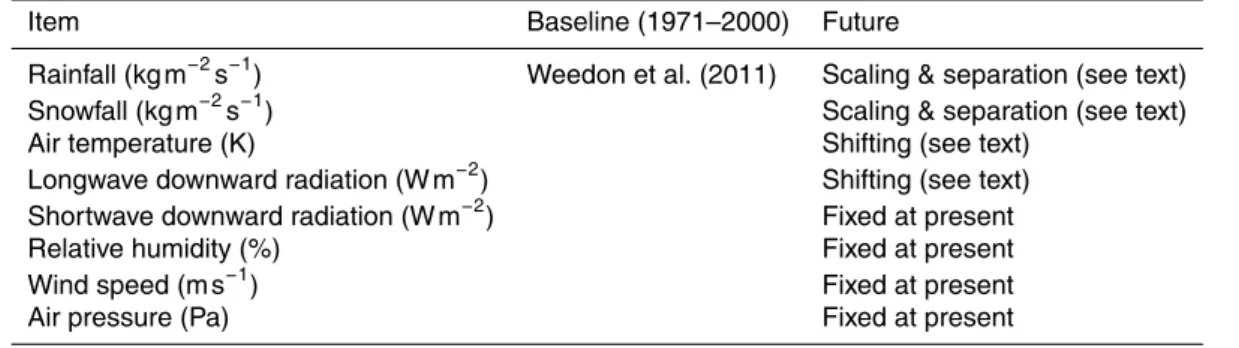
3.2 Meteorological data and scenarios

20

H08 requires the input of the eight meteorological variables listed in Table 1. For his-torical simulations, WATCH (Water and Global Change project) Forcing Data (Weedon

et al., 2011; hereafter WFD) was used. WFD covers the whole globe at a 0.5◦×0.5◦

spatial resolution. It covers the time period 1958–2001 at six-hourly intervals. We con-verted WFD data into daily intervals, and used 1971–2000 as the base period.

25

(10)

HESSD

9, 13933–13994, 2012

– Part 2

N. Hanasaki et al.

Tables Figures

◭ ◮

Back Close

Full Screen / Esc

Discussion

P

a

per

|

Dis

cussion

P

a

per

|

Discussion

P

a

per

|

Discussio

n

P

a

per

|

October 2012, the results of more than 40 global climate models (GCMs) are available via the internet. Although it is recommended to utilize all available GCMs to account for model uncertainty (Knutti et al., 2010), for practical reasons, we needed to restrict the number of GCMs used. We subjectively selected three GCMs, namely MIROC-ESM-CHEM (MIROC), HadGEM2-ES (HadGEM2), and GFDL-ESM2M (GFDL) (Table 2).

5

There is an open discussion regarding the selection of models (Knutti et al., 2010), but the models selected in this study are used in the Inter Sectoral Impact Model Intercop-marison Project (ISI-MIP; http://www.isi-mip.org/), which enabled cross checking with their results.

It is widely known that the output of GCMs contain systematic biases. In this study,

10

we corrected for the biases of air temperature, precipitation, and longwave downward radiation. Most of the earlier studies corrected only for air temperature and precipita-tion. We included longwave downward radiation, because this term shows an apparent increasing trend in all GCM projections. Moreover, this term is important in solving the surface energy balance. To remove bias, a shifting and scaling methodology was used

15

(e.g. Alcamo et al., 2007; Lehner et al., 2006).

T_{y, m, d}cor =T_{y, m, d}obs +Torgfuture,m−T org baseline,m

(3)

P_{y, m, d}cor =P_{y, m, d}obs ×

Porgfuture,m÷P org baseline,m

(4)

Lcor_{y, m, d}=Lobs_{y, m, d}×

Lorgfuture,m÷L org baseline,m

(5)

20

whereT, P, and L denote air temperature, precipitation, and longwave radiation,

re-spectively. The superscripts cor, obs, org denote bias-corrected, observation and orig-inal GCM values, respectively. The subscripts future, baseline, “y”, “m”, “d” indicate future period, retrospective period, year, month, and day, respectively. The upper bar indicates that the mean of thirty years’ records has been taken. After correcting for

25

(11)

HESSD

9, 13933–13994, 2012

– Part 2

N. Hanasaki et al.

Tables Figures

◭ ◮

Back Close

Full Screen / Esc

Discussion

P

a

per

|

Dis

cussion

P

a

per

|

Discussion

P

a

per

|

Discussio

n

P

a

per

|

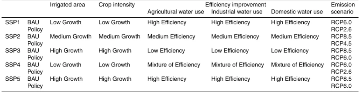
3.3 Non-meteorological data and scenarios

H08 requires the input of the non-meteorological variables listed in Table 3. For histori-cal simulations, we used published datasets, which represent the period circa 2000. For future simulations, we used scenarios developed in the accompanying paper (Hanasaki et al., 2012) for irrigated area, crop intensity, irrigation efficiency, and potential

indus-5

trial and domestic water withdrawal demand. Due to a lack of available information, the other variables were kept at present levels.

Crop type was set by using the crop type data of Monfreda et al. (2008). They pro-vided the areal fraction of 175 crop types, but we used only 19 that are commonly culti-vated worldwide. H08 is able to simulate up to two crops per year (multiple-cropping is

10

common in tropics), but needs to select only one crop type per grid cell during a crop-ping period (from planting to harvesting date). Here we assumed that the crop type of the largest fraction is planted in the first crop, and that of the second largest is in the second. We fixed the crop type throughout the 21st century, because of a lack of available data. This might be unrealistic because farmers would change the crop type

15

to adapt to a changing climate and the demands of the crop. Because it is beyond the scope of this study to discuss future agricultural practices and food production, we left the crop type scenario until such time as the integrated assessment community can provide relevant scenarios and guidelines (see also the discussion in Sects. 3 and 7 of Hanasaki et al., 2012).

20

Potential water withdrawal demand for industrial and municipal use is provided as the withdrawal base. In order to convert it into a consumption (i.e. evaporation) base, we used the factor 0.10 and 0.15, respectively, from the work of Shiklomanov (2000). Po-tential water consumption demand for agricultural use is simulated by H08. In order to convert it into the withdrawal base, we used the irrigation efficiency scenario developed

25

(12)

HESSD

9, 13933–13994, 2012

– Part 2

N. Hanasaki et al.

Tables Figures

◭ ◮

Back Close

Full Screen / Esc

Discussion

P

a

per

|

Dis

cussion

P

a

per

|

Discussion

P

a

per

|

Discussio

n

P

a

per

|

3.4 Simulation settings

We configured models and set up a simulation protocol as shown in Tables 4 and 5. We configured H08 in two forms, first for naturalized simulation (NAT), using only land surface and river sub models, and second for human simulation (HUM), using all six sub models. The NAT was used to assess a situation that assumed there was no

5

human activity at all during the simulation periods, to evaluate the impact of climate change on the hydrological cycle. The HUM was used to assess water scarcity.

For the baseline period (1971–2000), two simulations were conducted with a natu-ralized configuration (NAT-Baseline) and human configuration (HUM-Baseline).

For the future periods, we conducted four simulations: naturalized configuration

(NAT-10

FUT), human configuration fixing non-meteorological variables at circa 2000 (HUM-Fix), using the SSPs without a climate policy (business as usual; HUM-BAU), and using the SSPs with a climate policy (HUM-Policy). Three simulation periods were set, 2011– 2040, 2041–2070 and 2071–2100.

The NAT-Future simulation was conducted to analyze the hydrological response to

15

climate change. H08 was set to a naturalized configuration, and future meteorological data (Eqs. 3–5) were prepared for three RCPs (RCP2.6, 4.5, 8.5) and three GCMs (MIROC, HadGEM2, GFDL).

The HUM-Fix simulation was conducted to analyze the magnitude of change in wa-ter availability and use due to climate change, excluding the effect of socio-economic

20

changes. Three RCPs were used for three GCMs, but non-meteorological variables were fixed at the baseline period.

The HUM-BAU simulation was conducted to analyze water availability and scarcity under a business as usual situation, with no climate policy. All five of the SSP scenarios were used. For each scenario an RCP was selected that was compatible with the

25

(13)

HESSD

9, 13933–13994, 2012

– Part 2

N. Hanasaki et al.

Tables Figures

◭ ◮

Back Close

Full Screen / Esc

Discussion

P

a

per

|

Dis

cussion

P

a

per

|

Discussion

P

a

per

|

Discussio

n

P

a

per

|

The HUM-Policy simulation was conducted to evaluate how climate policies alleviate water scarcity for each SSP. All five of the SSP scenarios were used. In this study, climate policy switches RCPs into lower levels. For each scenario an RCP was selected that was compatible with an emission path including a climate policy (Table 5, see also Fig. 2 of Hanasaki et al., 2012). Again note that the consistency of RCPs, SSPs,

5

and the policy scenarios are not fully assured. Climate policy simulations in this study were conducted primarily to determine the response to a lower level of climate change. Although not available as of October 2012, a climate policy scenario called Shared Policy Assumptions (SPA) is under discussion (Kriegler et al., 2012).

4 Results and discussion part 1: NAT-Future and HUM-Fix simulations

10

In this section, we analyze the results of the NAT-Future and HUM-Fix simulations and compare them with the NAT-Baseline and HUM-Baseline simulations, respectively. The results of the HUM-Baseline simulation are shown in Fig. 2. As can be seen from Table 4, non-meteorological data, such as population and land use, was not used or fixed at the baseline period in these settings. This section provides basic information

15

regarding the response of hydrology and the water scarcity index to climate change. A consideration of both climate and socio-economic change are critical for understand-ing the results of a water scarcity assessment as described in the next section.

4.1 Climate change

First, we focus on the change in air temperature, which indicates the magnitude of

20

climate change, and then the change in precipitation, which directly impacts on water resources and potential agricultural water consumption demand.

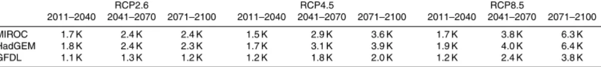
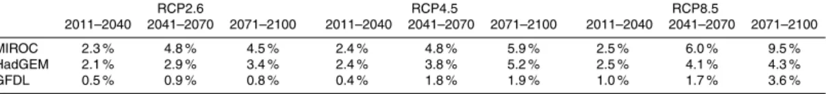
Tables 6 and 7 show the changes in mean global terrestrial (i.e. land only) temper-ature and precipitation, respectively. The projected rise of global terrestrial mean tem-perature in 2071–2100, compared to the baseline period (1971–2000), was 1.2–2.4 K

(14)

HESSD

9, 13933–13994, 2012

– Part 2

N. Hanasaki et al.

Tables Figures

◭ ◮

Back Close

Full Screen / Esc

Discussion

P

a

per

|

Dis

cussion

P

a

per

|

Discussion

P

a

per

|

Discussio

n

P

a

per

|

(RCP 2.6), 2.0–3.9 K (RCP 4.5), and 3.8–6.4 K (RCP 8.5). Global mean precipitation increased by 0.8–4.5 %, 1.9–5.9 %, and 3.6–9.5 %, respectively. The MIROC projection produced the largest increases among the three models. HadGEM2 projected a similar temperature rise to MIROC, but the change in precipitation was slightly smaller. GFDL projected the least change in both temperature and precipitation among the three

mod-5

els, being less than half of MIROC and HadGEM2.

Figures 3 and 4 show the geographical patterns of global temperature rise and precipitation changes projected by MIROC. Only the results of MIROC are used for discussion of geographical patterns hereafter, because the model shows the largest change among the three used. From Figs. 3 and 4, it can be clearly seen that the

spa-10

tial pattern of change is similar among periods and RCPs, and only the magnitude of change increases as time and radiative forcing increases from a macroscopic perspec-tive. Although the other two models produced different spatial patterns and magnitudes, a generally consistent pattern was identified, where temperature in the northern high latitudes increased rapidly, as compared to the low latitudes. Precipitation decreased

15

in semi arid areas such as near the Mediterranean Sea, central to western mid-latitude North America, southern Africa and south eastern South America. One important

find-ing, as shown by Tables 6–7 and Figs. 3–4 is that there is no clear difference when

using RCP2.6, RCP4.5, and RCP8.5 in 2011–2040. There are distinct differences after

2041–2070 in terms of both the mean global changes and geographical patterns.

20

4.2 Hydrological change

Next, the change in mean estimated annual runoffis discussed. Mean annual runoffis

a key variable in the assessment of water resources, because it corresponds to regional renewable water resources. We focused on the results of the NAT-Future simulation, which displayed a hydrological response to climate change.

25

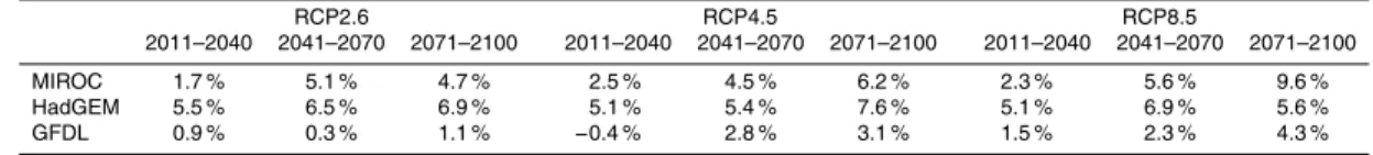
Table 8 shows the estimated change in runoff for each scenario and period. The

(15)

HESSD

9, 13933–13994, 2012

– Part 2

N. Hanasaki et al.

Tables Figures

◭ ◮

Back Close

Full Screen / Esc

Discussion

P

a

per

|

Dis

cussion

P

a

per

|

Discussion

P

a

per

|

Discussio

n

P

a

per

|

example, MIROC projected the largest increase in runoff among the three models,

which is consistent with the change in precipitation.

Figure 5 shows the geographical pattern of the change in runoff. Although the

pat-tern of runoff changes (i.e. red-blue distribution) was similar to that of precipitation changes (Fig. 4), there was a much stronger contrast with the regional pattern (the

5

color schemes are identical for Figs. 4 and 5). Generally, runoffincreased in the north-ern high latitudes and decreased in the mid-latitudes. The figure indicates that, for

MIROC under the RCP8.5 scenario, the mean annual runoffin 2071–2100 was altered

by more than 10 % from the baseline period, in almost all regions of the world.

4.3 Potential agricultural water withdrawal demand

10

Next, the simulated potential agricultural water withdrawal demand is discussed using the results of HUM-Fix simulations. Potential agricultural water consumption demand is defined as the irrigation water required to maintain soil moisture in the top 1 m of irrigated cropland at 75 % (100 % for rice) during cropping periods assuming water is available anytime and anywhere. The results were converted into the withdrawal

15

base by using water use efficiency which is the ratio of water consumed over water

withdrawn including return flow and delivery loss. H08 simulates the former, while the latter is widely recorded allowing us to convert water consumed into water withdrawn.

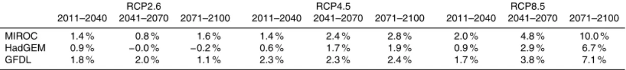
Table 9 shows the projected change in global total agricultural water demand. The

projected ranges for RCP2.6, RCP4.5, and RCP8.5 were−0.2–1.6 %, 1.9–2.8 %, and

20

6.7–10.0 %, respectively, in 2071–2100. This indicates that the total global potential agricultural water withdrawal demand increases in almost all scenarios. This is con-sistent with the findings of D ¨oll (2002) who reported the results of similar numerical

experiments. The di_fference among models and scenarios was small in 2011–2040,

but became more distinct after 2041–2070.

25

Figure 6 shows the change in the mean annual potential agricultural water withdrawal

demand projected by MIROC. In 2011–2040, the change was no more than±10 % in

(16)

HESSD

9, 13933–13994, 2012

– Part 2

N. Hanasaki et al.

Tables Figures

◭ ◮

Back Close

Full Screen / Esc

Discussion

P

a

per

|

Dis

cussion

P

a

per

|

Discussion

P

a

per

|

Discussio

n

P

a

per

|

for the Asian monsoon regions and Australia. In 2071–2100 and particularly for the results using RCP8.5, many regions displayed an increase or decrease larger than

±10 %. This pattern is primarily explained by the change in precipitation with irriga-tion water demand increasing in regions receiving less precipitairriga-tion and vice versa. In addition to precipitation, higher temperatures and downward longwave radiation also

5

contribute to an increase in the potential evapotranspiration, which eventually leads to a higher water requirement.

4.4 Withdrawal to water resources ratio

Water scarcity was assessed using the WWR. The index is expressed as the mean annual total withdrawal (W) over the mean annual river discharge (Q). This index is

10

widely used because of its intuitiveness and simplicity. We focused on both the index itself (W/Q) and the so-called water stressed population, which is defined here as the total population living in grid cells where the index exceeds 0.4.

Table 10 shows the total global water stressed population and highlights two inter-esting findings. First, the estimated water stressed population varied only marginally

15

across all scenarios. Second, there was no clear relationship between the water stressed population and either time or GHG emissions (i.e. RCPs). In some simula-tions, water stress decreased as time progressed (e.g. when using RCP2.6 in MIROC the water stressed population in 2041–2070 was smaller than in 2011–2040) or as GHG emissions increased (e.g. in 2041–2070 of MIROC, the water stressed

popula-20

tion using RCP4.5 was smaller than when using RCP2.6).

The minor changes in the water stressed population can be primarily explained by

the robustness of the index. In the HUM-Fix simulation, we fixed W (the numerator

of Eq. 1). Agricultural water withdrawal was also affected by climate change but the

change was small. Therefore, Q (the denominator) had the primary role in this

as-25

sessment. Although climate change affected the hydrological cycle globally, the dry

(17)

HESSD

9, 13933–13994, 2012

– Part 2

N. Hanasaki et al.

Tables Figures

◭ ◮

Back Close

Full Screen / Esc

Discussion

P

a

per

|

Dis

cussion

P

a

per

|

Discussion

P

a

per

|

Discussio

n

P

a

per

|

populated grid cell in an arid region generated a water stressed population in all sce-narios. The estimation of the total global water stressed population was considered to be robust due to these factors.

To analyze the change in the water stressed population, we focused on the change in WWR. Figure 7 shows the geographical pattern of changes in the WWR. We

de-5

fined the change as the ratio of WWR of the future period to the baseline, because WWR takes a wide range (almost zero in wet unpopulated regions to thousands in dry

populated regions). The positive and negative signs basically correspond to the runoff

scenario from Fig. 5. WWR increased where runoff decreased and vice versa. Note

that the change was shifted toward the negative (i.e. water scarcity) direction, because

10

global agricultural water withdrawal increased slightly (Fig. 6).

Table 10 shows the population living in the grid cells where water stress conditions improved (WWR decreased) or worsened (WWR increased). Again some interesting results were observed. Water stress conditions improved for more than half of the pop-ulation. This may indicate that climate change alleviates water scarcity or an increase

15

in mean annual runoff may improve the availability of water. These issues are further

investigated in the next subsection.

4.5 Cumulative withdrawal to demand ratio

In order to further investigate water scarcity following climate change, the CWD is used in this section. The index is expressed as the accumulation of daily withdrawal from

20

rivers over the accumulation of daily potential water consumption demand. This index is useful for determining whether water is available when it is needed, taking into account the seasonality of both water availability and use. Excess water (e.g. flood water in wet seasons) is not considered to be available. We focused on both the index itself and the water stressed population, which is defined here as the total population living in a grid

25

where the index falls below 0.5.

(18)

HESSD

9, 13933–13994, 2012

– Part 2

N. Hanasaki et al.

Tables Figures

◭ ◮

Back Close

Full Screen / Esc

Discussion

P

a

per

|

Dis

cussion

P

a

per

|

Discussion

P

a

per

|

Discussio

n

P

a

per

|

emissions, i.e. climate change degraded water availability. However, as with the WWR results, the water stressed population did not change significantly among scenarios. This is due to the same reasons we discussed in the previous subsection: regions with a strong seasonality in both water availability and use retain these features under various climate change scenarios.

5

Figure 8 shows the global pattern of differences in the CWD. The figure shows the

difference, not the actual ratio, because the CWD ranges between 0 and 1 and has

a physical meaning by showing the fraction of fulfillment of the local potential water consumption demand. In many parts of the world, the water stress increased. The pattern differs from the pattern of runoff change (Fig. 5), indicating that although the

10

total annual runoffincreased, water resources are not available when they are needed.

For example, while the mean annual runoffincreased in the Sahel regions, CWD

de-creased (i.e. water stress increases). The increase in runoffin the wet seasons did not contribute to water resources in dry seasons, and the gap between water availability and use in dry seasons worsened. The results imply that the increase in mean annual

15

runoffdid not alleviate water scarcity in these regions.

Table 11 shows the population living in the grid cells where water stress conditions

improved (CWD increased) or worsened (CWD decreased). The population suffered

from an increase in water stress over time and with increased GHG emissions.

Al-though total global runoff increased, the results indicate that less than 30 % of the

20

population benefitted in terms of improved water availability.

5 Results and discussion part 2: HUM-BAU and HUM-Policy simulations

In this section, we analyze the results of the HUM-BAU and HUM-Policy simulations in contrast with the HUM-Baseline simulation. We mainly focused on the relationship between the SSPs and water scarcity.

(19)

HESSD

9, 13933–13994, 2012

– Part 2

N. Hanasaki et al.

Tables Figures

◭ ◮

Back Close

Full Screen / Esc

Discussion

P

a

per

|

Dis

cussion

P

a

per

|

Discussion

P

a

per

|

Discussio

n

P

a

per

|

5.1 Potential agricultural water withdrawal demand

Table 12 shows the total global potential agricultural water withdrawal demand. The

range among the SSPs was as much as 3154–8595 km3yr−1 in 2071–2100. In the

HUM-BAU simulation, SSP3 produced the largest potential agricultural water with-drawal demand, followed by SSP5, SSP2, SSP4, and SSP1. Of the three GCMs,

5

MIROC projected the largest demand but the differences among the three GCMs were

relatively small. The HUM-Policy simulation systematically decreased the projection of potential agricultural water withdrawal demand in all SSPs and GCMs, as compared to the HUM-BAU simulation, but the change was only a few percent.

The differences in the results can be explained by the simulation settings

summa-10

rized in Table 5. Irrigation growth scenarios and irrigation water efficiency scenarios have an important role in projecting potential agricultural water withdrawal demand. It is clear that the combination of low growth and high efficiency (SSP1) resulted in the least

demand, and high growth and low efficiency (SSP3) resulted in the greatest demand,

with the mid-growth and mid-efficiency scenario (SSP2) producing intermediate levels

15

of demand. The setting of SSP4 is similar to SSP1, except for the irrigation efficiency scenario. SSP4 assumes that irrigation efficiency is high in OECD countries and low in non-OECD countries. Because the irrigation equipped area is predominantly located in non-OECD countries, this assumption contributes to the increased potential agricul-tural water withdrawal demand when using SSP4, as compared to SSP1. Similarly, the

20

irrigation growth in SSP5 was identical to that of SSP3 but, due to improvements in

efficiency, the increase in water demand for SSP5 was much more restricted than for

SSP3. In addition to the irrigation growth and efficiency scenarios, the climate scenar-ios are also different for each SSP. However, as discussed in the previous chapter and as shown in Table 9, the effect produced a difference of only few percent at most. This

25

also explains why the differences in the HUM-BAU and HUM-Policy simulations were

(20)

HESSD

9, 13933–13994, 2012

– Part 2

N. Hanasaki et al.

Tables Figures

◭ ◮

Back Close

Full Screen / Esc

Discussion

P

a

per

|

Dis

cussion

P

a

per

|

Discussion

P

a

per

|

Discussio

n

P

a

per

|

Table 13 shows the total global potential water withdrawal demand for all sectors. We added the global potential agricultural water withdrawal (Table 12) and industrial and municipal water withdrawal (Tables 10 and 11 of Hanasaki et al., 2012). As with the global agricultural water withdrawal, SSP3 produced the largest demand, followed by SSP5, SSP2, SSP4, and SSP1. SSP3 produced levels of demand two and three times

5

higher than SSP1 in 2041–2070 and 2071–2100, respectively.

Figure 9 shows the geographical pattern of change in potential agricultural water withdrawal demand. For SSP1, water demand displayed only small changes and even decreased in some regions of the Northern Hemisphere. For SSP4, which assumes low irrigation water use efficiency in non-OECD countries, irrigation water demand

in-10

creased in those countries. For SSP2 and SSP3 potential demand for most regions increased, particularly in South Asia and Eastern South America.

5.2 Water scarcity assessment using the Cumulative Withdrawal to Demand (CWD) ratio

In this section, water scarcity is assessed using the CWD ratio for the HUM-BAU and

15

HUM-Policy simulations. WWR has been widely used in previous studies, but it can be misleading when interpreting the impact of climate change on water scarcity, as discussed in Sects. 4.4 and 4.5. The results using the WWR are given in Appendix A, for readers’ convenience.

Table 14 shows the water stressed population using the CWD. The water stressed

20

population was largest for SSP3, followed by SSP2, SSP5, SSP4, and SSP1. Taking into account the differences of population, the percentage of the total global population that is projected to become water stressed was largest for SSP3, followed by SSP5, SSP2, SSP4, and SSP1. This order is identical to that observed for the total water demand.

25

(21)

HESSD

9, 13933–13994, 2012

– Part 2

N. Hanasaki et al.

Tables Figures

◭ ◮

Back Close

Full Screen / Esc

Discussion

P

a

per

|

Dis

cussion

P

a

per

|

Discussion

P

a

per

|

Discussio

n

P

a

per

|

of climate change and population growth. First, as already shown in Table 11, climate change degraded the water availability of 67 % of the global population. Moreover, the increase in population further increased the water stressed population, negating the impact of a decrease in total water demand (Table 13).

The range in the size of water stressed populations among SSPs that took both

wa-5

ter use and climate scenarios into account (Table 14) was much greater than that of the HUM-Fix simulation, which only took a climate scenario into account (Table 11). This indicates that a water stressed population is much more sensitive to a water use (or socio-economic) scenario than climate change. Note that the water stressed pop-ulation increased in all scenarios, including SSP1 in which total global water demand

10

decreases. This is mainly because of the increase in population, particularly in devel-oping countries.

Figure 10 shows the geographical pattern of differences in the CWD. It is clear that in all SSPs water stress conditions increase in the Sahel and southern Africa. This is due to the increase in potential water consumption demand from all sectors. In

addi-15

tion to the agricultural water demand, substantial growth in electricity production and population led to an increase in industrial and municipal water demand. For SSP1, the water availability of other regions was less severely affected. The situation is similar in SSP4. In contrast, for SSP2 and SSP3, water stress conditions increase in populated areas such as northern to central China, the Mediterranean, and eastern to central

20

North America.

The geographical pattern of Fig. 10 can be explained by the change in the CWD influenced by the different climate scenarios (Fig. 8) and water use reflecting different socio-economic scenarios (Fig. 9). For SSP1, because water use is not increasing significantly at the global level, the results are similar to Fig. 8. In contrast, for SSP3,

25

(22)

HESSD

9, 13933–13994, 2012

– Part 2

N. Hanasaki et al.

Tables Figures

◭ ◮

Back Close

Full Screen / Esc

Discussion

P

a

per

|

Dis

cussion

P

a

per

|

Discussion

P

a

per

|

Discussio

n

P

a

per

|

Oceania, Japan, EU, rest of Europe including the Baltic countries, and Former Soviet Union excluding the Baltic countries). The number of water stressed populations in the last five regions is merged in Fig. 11, because each number was small compared to the other regions. Water stressed regions are unevenly distributed in the world. The number of water stressed populations was highest in Africa, India, China, and rest

5

of Asia throughout the century. The largest growth in water stressed populations was seen in Africa.

Figure 12 shows the percentage of the global population in specific water stress cate-gories. We subdivided the population of the world according to two factors. First, all grid

cells were subdivided into three according to the change in CWD (∆CWD). We used

10

the term Significant Degradation for grid cells where_∆CWD<−0.05, Moderate

Degra-dation where−0.05≤_∆CWD<0, and Alleviation or no change where 0≤_∆CWD.

Sec-ond, each category was further subdivided into three by the CWD. We used the term

Highly Stressed for CWD<0.5, Moderately Stressed for 0.5≤CWD<0.8, and Less

Stressed for 0.8≤CWD. The results clearly showed that an alleviation of water stress

15

conditions were projected for only a limited proportion of the global population, (i.e. CWD decreases compared with baseline period, shown in blue) in all of the SSPs. For most people in the world, water stress conditions increase due to global climate change

(red and orange). However, populations suffering from severe degradation of the CWD

(_∆CWD<−0.05) vary among the scenarios. For example, in SSP1 around 30 % of the

20

global population suffer from severe degradation (shown as red), whereas for SSP3

the value is around 60 % in 2041–2070. Fewer populations suffer from severe water

scarcity when a climate policy is taken into consideration, especially in 2071–2100.

5.3 Implications

Based on the findings above, particularly from Figs. 11 and 12, we derived the

implica-25

tions of each SSP.

(23)

HESSD

9, 13933–13994, 2012

– Part 2

N. Hanasaki et al.

Tables Figures

◭ ◮

Back Close

Full Screen / Esc

Discussion

P

a

per

|

Dis

cussion

P

a

per

|

Discussion

P

a

per

|

Discussio

n

P

a

per

|

least climate change and the smallest increase in water use. For example, we adopted RCP2.6 as a climate scenario with the adoption of a climate policy that was intended to stabilize the global mean air temperature around+2◦C from the industrial revolution level. For the water use scenario, we adopted the lowest projection of irrigation area expansion from published reports (+0.06 % yr−1; see Table 5 and Table 2 of Hanasaki

5

et al., 2012) and the highest rate of improvement in irrigation water use efficiency. The

efficiency improvement of industrial water use was taken from the observed rates in

highly water efficient countries in the latter half of the 20th century. Municipal water

withdrawal decreases toward per capita municipal water use of 200 L day−1 globally.

Consequently, the projected total water withdrawal decreased slightly, as compared to

10

the baseline period. Although the resulting water scarcity was by far the lowest among the SSPs, the results indicated that global water scarcity in SSP1 increased, as com-pared to the baseline period. This implies that even for one of the most optimistic sce-nario combinations, pressure on water resources will continue throughout the current century.

15

SSP2 (middle of the road) depicts a future world where the socio-economic trends of recent decades continue. For this scenario we combined moderate scenarios and options. We confirmed that our projected water withdrawal largely agreed with earlier reports that assumed the continuation of current trends (Hanasaki et al., 2012). This is consistent with the key concept of SSP2, which is a future world considered to be

20

“dynamic as usual”. Under these assumptions, water use continuously increased and consequently water stress also increased in many parts of the world. Figure 11 indi-cates that the total global water stressed population nearly doubled by the middle of the century and continued to increase toward the end of the century.

SSP3 (fragmented world) depicts a future world of extreme poverty and a rapidly

25

(24)

HESSD

9, 13933–13994, 2012

– Part 2

N. Hanasaki et al.

Tables Figures

◭ ◮

Back Close

Full Screen / Esc

Discussion

P

a

per

|

Dis

cussion

P

a

per

|

Discussion

P

a

per

|

Discussio

n

P

a

per

|

population had nearly tripled by the end of the century. Around 50 % of the total pop-ulation was projected to live in grid cells categorized as Highly Stressed (0.5<CWD) and Significant Degradation (∆CWD<−0.05; Table 14).

SSP4 (inequality) depicts a highly unequal future world. The water use scenario was similar to that of SSP1, but the improvements in e_fficiency were assumed to be low for

5

non-OECD countries. The results showed similar water stress characteristics to SSP1, but much more severe for developing countries, particularly in Africa (Fig. 11).

SSP5 (conventional development) depicts a future world of robust economic growth based on the continued exploitation of fossil fuels. Its water use scenario was similar to that of SSP3, but the improvement in efficiency was high for all countries, as inferred

10

from the narrative scenario of SSP5. Together with the lower population growth, the water stressed population was lower than in SSP3, but the proportion of the global

population suffering from reduced water availability was almost the same as in SSP3.

Because the available water was much less than the potential water consumption de-mand, it was implied that social activity could be restricted by water shortages. This

15

implied the need for the development of extra water resources, such as increasing water storage capacity, abstracting more groundwater or increasing desalination.

6 Uncertainty

6.1 Climate scenario

In this study, we used three GCMs, although more than 40 GCMs are readily available

20

(Taylor et al., 2012). There is a need to increase the number of GCMs in order to cover the uncertainty of climate projections. We selected three GCMs subjectively. Although there is no established methodology to prioritize the available GCMs (Knutti et al., 2010), performance metrics for GCMs (e.g. Gleckler et al., 2008) would be useful to ensure that the selection process is less subjective.

(25)

HESSD

9, 13933–13994, 2012

– Part 2

N. Hanasaki et al.

Tables Figures

◭ ◮

Back Close

Full Screen / Esc

Discussion

P

a

per

|

Dis

cussion

P

a

per

|

Discussion

P

a

per

|

Discussio

n

P

a

per

|

When preparing the climate scenario, we adopted a shifting and scaling method (Lehner et al., 2006) to remove the biases of the GCMs. This was computationally efficient, because only the mean monthly difference was added or multiplied to the ret-rospective time series of meteorological forcing data. Moreover, because of this sim-plicity, the climate scenario is consistent with the baseline period, and produces stable

5

results. However, neglecting the temporal variability of change is a widely recognized shortcoming of this method. In some cases, this might underestimate (or overestimate) the risk of drought and water shortage. New techniques of GCM bias correction have been devised and have been applied in global studies. For example, Piani et al. (2010) developed a global daily climate scenario for three CMIP3 GCMs. Although it is very

10

labor intensive to develop such techniques, their adoption is essential.

6.2 Socio-economic and water use scenario

Because the uncertainty associated with the socio-economic and water use scenario is described in the accompanying paper (Hanasaki et al., 2012), we only summarize the key points here. First, we used AIM-SSP, which provides preparatory quantitative

15

scenarios for the SSPs from an integrated assessment by the Asia-Pacific Integrated Model (Kainuma et al., 2002). Official SSP products will be released in the near future, and may vary from the current AIM-SSP. Second, the irrigation growth scenario was developed from a literature review that was independent of any food-related SSP fac-tors. As discussed in detail in the accompanying paper, this is primarily due to the lack

20

of information regarding how to link food and irrigation. An integrated model that links crops, water, and land (e.g. Lotze-Kampen et al., 2008) is likely to establish a more comprehensive and consistent scenario. Third, we used a simplistic model to estimate industrial and municipal water use. Progress in this area of modeling has long been ob-structed by a lack of data, but further efforts are needed. The results of water resource

25

(26)

HESSD

9, 13933–13994, 2012

– Part 2

N. Hanasaki et al.

Tables Figures

◭ ◮

Back Close

Full Screen / Esc

Discussion

P

a

per

|

Dis

cussion

P

a

per

|

Discussion

P

a

per

|

Discussio

n

P

a

per

|

6.3 Combination of scenarios

In this study, many independent scenarios were combined, namely the SSPs (socio-economic scenarios), our water use scenario (Hanasaki et al., 2012), RCPs (GHG emission scenario) and CMIP5 (climate scenario). This allowed us to achieve our pri-mary objective, i.e. to develop a water use scenario compatible with the SSPs for use

5

in global water scarcity assessments. Here two points should be noted. First, because each scenario was independently developed, consistency among the scenarios was unachievable. Combinations of scenarios and options were decided on a largely ar-bitrary basis, because there were neither clear guidelines nor many previous studies that were available. To improve consistency, further interdisciplinary modeling e_fforts

10

are needed to develop an integrated model that incorporates all of these aspects.

Sec-ond, the feasibility of each scenario could be different. For example, SSP1 and SSP3

have been developed to depict high and low-end scenarios, which might be perceived to be less realistic than the “middle of the road” scenario depicted in SSP2. Each sce-nario should be considered to be an option and not a prediction of the future.

15

6.4 Models

As described earlier, the H08 model has been applied to a number of studies and has been used in international model comparison projects. All of the results indicate that the performance of the model is at the current state-of-the-art level. However, it should be noted that the basin and grid-cell level results include uncertainties because

20

basin-wise fine parameter tuning has not been carried out (this is a challenging task; see Hanasaki et al., 2008a for detailed discussion). Model inter comparison projects for climate change simulation have been undertaken (e.g. WaterMIP; Hagemann et al., 2012; ISI-MIP, http://isi-mip.org/), and are useful for quantifying the uncertainties of each participating model.

25

(27)

HESSD

9, 13933–13994, 2012

– Part 2

N. Hanasaki et al.

Tables Figures

◭ ◮

Back Close

Full Screen / Esc

Discussion

P

a

per

|

Dis

cussion

P

a

per

|

Discussion

P

a

per

|

Discussio

n

P

a

per

|

1.0×109m3of storage capacity were taken into account. This assumption was useful

when investigating the impact of climate change on daily water availability: the change in water balance and flow regime is directly reflected in the CWD water scarcity index. Although river water accounts for 78 % of total global water withdrawal (FAO, 2011), in reality, river water is one of many sources of water. Groundwater is an important

5

source of water, and has been reported to be vulnerable to climate change due to predicted decreases in recharge (D ¨oll et al., 2009). Reservoirs with a storage capacity of less than 1.0×109m3 also have an important role by storing water in wet periods and carrying it over into dry seasons. Although these are important sources of water we excluded them for two reasons. First, a scaling problem hampers the modeling.

10

The groundwater dynamics take place at a much finer scale than the current spatial resolution of 0.5◦×0.5◦. Similarly, in some cases, dozens of reservoirs are located in

a particular grid cell. Parameterization of these is still in its infancy (Hanasaki et al., 2010). Second, preparing scenarios for these terms is very challenging and may be impossible.

15

6.5 Water scarcity indexes

We assessed water scarcity globally using two indexes, WWR and CWD. WWR has been widely used in the previous assessments. The results should be considered with care. As we have discussed in previous sections, the nature of these indexes shows an

alleviation of water stress when the mean annual runoffincreases. Mean annual runoff

20

could be increased by rainfall in a rainy season or under extreme precipitation. These increases are usually difficult to utilize as water resources (Kundzewitz et al., 2007).

CWD overcomes the key shortcoming of WWR. It directly accounts for the fulfill-ment of daily potential water consumption demand, which excludes flooding or

ex-treme runofffrom available water resources. However, two strong assumptions should

25