doi:10.5194/cp-12-2271-2016
© Author(s) 2016. CC Attribution 3.0 License.
The simulated climate of the Last Glacial Maximum and insights
into the global marine carbon cycle
Pearse J. Buchanan1,2,3, Richard J. Matear2,3, Andrew Lenton2, Steven J. Phipps1, Zanna Chase1, and David M. Etheridge4
1Institute for Marine and Antarctic Studies, University of Tasmania, Hobart, Tasmania, Australia
2CSIRO Oceans and Atmosphere, CSIRO Marine Laboratories, G.P.O. Box 1538, Hobart, Tasmania, Australia 3ARC Centre of Excellence in Climate System Science, University of Tasmania, Hobart, Australia
4CSIRO Ocean and Atmosphere, Aspendale, Victoria, Australia
Correspondence to:Pearse J. Buchanan ([email protected])
Received: 1 July 2016 – Published in Clim. Past Discuss.: 11 July 2016
Revised: 21 November 2016 – Accepted: 27 November 2016 – Published: 22 December 2016
Abstract.The ocean’s ability to store large quantities of
car-bon, combined with the millennial longevity over which this reservoir is overturned, has implicated the ocean as a key driver of glacial–interglacial climates. However, the com-bination of processes that cause an accumulation of carbon within the ocean during glacial periods is still under debate. Here we present simulations of the Last Glacial Maximum (LGM) using the CSIRO Mk3L-COAL (Carbon–Ocean– Atmosphere–Land) earth system model to test the contri-bution of physical and biogeochemical processes to ocean carbon storage. For the LGM simulation, we find a signif-icant global cooling of the surface ocean (3.2◦C) and the expansion of both minimum and maximum sea ice cover broadly consistent with proxy reconstructions. The glacial ocean stores an additional 267 Pg C in the deep ocean rel-ative to the pre-industrial (PI) simulation due to stronger Antarctic Bottom Water formation. However, 889 Pg C is lost from the upper ocean via equilibration with a lower at-mospheric CO2 concentration and a global decrease in ex-port production, causing a net loss of carbon relative to the PI ocean. The LGM deep ocean also experiences an oxy-genation (>100 mmol O2m−3) and deepening of the cal-cite saturation horizon (exceeds the ocean bottom) at odds with proxy reconstructions. With modifications to key bio-geochemical processes, which include an increased export of organic matter due to a simulated release from iron lim-itation, a deepening of remineralisation and decreased inor-ganic carbon export driven by cooler temperatures, we find that the carbon content of the glacial ocean can be
suffi-ciently increased (317 Pg C) to explain the reduction in at-mospheric and terrestrial carbon at the LGM (194±2 and 330±400 Pg C, respectively). Assuming an LGM–PI differ-ence of 95 ppmpCO2, we find that 55 ppm can be attributed to the biological pump, 28 ppm to circulation changes and the remaining 12 ppm to solubility. The biogeochemical modifi-cations also improve model–proxy agreement in export pro-duction, carbonate chemistry and dissolved oxygen fields. Thus, we find strong evidence that variations in the oceanic biological pump exert a primary control on the climate.
1 Introduction
interglacial changes in atmospheric CO2 (Broecker, 1982; Skinner et al., 2015; Wilson et al., 2015). However, identify-ing the combination of mechanisms that drove a flux of car-bon into the ocean during glacial periods remains a funda-mental and largely unresolved problem.
If we first consider only physical changes, a net influx of CO2caused by cooling is a feature of the glacial ocean. However, the increase in solubility attributed to cooling is partially offset by increased salinity due to a lower sea level (Siddall et al., 2003), so that the contribution of sol-ubility changes is estimated at ∼13 ppm of the total 80– 100 ppm CO2drawdown (Sigman and Boyle, 2000; Kohfeld and Ridgwell, 2009). Therefore, other physical changes as-sociated with a glacial climate, notably changes to the large-scale circulation and sea ice fields (Stephens and Keeling, 2000), may make a considerable contribution to carbon se-questration. Proxy evidence (Curry and Oppo, 2005; Dup-lessy et al., 1988; McManus et al., 2004; Oliver et al., 2010; Skinner et al., 2010) and model experiments (Brovkin et al., 2007; Hain et al., 2010; Menviel et al., 2012; Watson and Naveira Garabato, 2006) of the glacial climate have shown that a greater proportion of the deep ocean was dominated by southern source waters (see Adkins, 2013, for a review). The existence of this glacial-type circulation has been connected to an expanded sea ice field (Ferrari et al., 2014). An expan-sion of southern source waters throughout the deep ocean and an expanded sea ice field are now considered to be primary candidates for carbon sequestration during glacial climates (Adkins, 2013).
However, the most promising explanations of the glacial decline in atmospheric CO2 involve changes to ocean pro-ductivity in concert with reorganisations of the global over-turning circulation (Hain et al., 2010; Gottschalk et al., 2016). An increased glacial productivity, first proposed by Broecker (1982) and explored by Archer et al. (2000) by in-creasing the global nutrient inventory, is now an established feature of the subantarctic zone due to enhanced aeolian de-position of iron (Martinez-Garcia et al., 2014). The Southern Ocean exerts a strong control on atmospheric CO2through its direct connection with deep waters (Marinov et al., 2006), and enhanced productivity in this zone is thus a prime candi-date for explaining a fraction of the glacial–interglacial CO2 difference.
In numerous other regions, however, productivity appears to have been reduced during glacial climates. The affected regions include waters south of the Antarctic Polar Front (Francois et al., 1997; Jaccard et al., 2013), the North Pa-cific (Crusius et al., 2004; Jaccard et al., 2005; Kohfeld and Chase, 2011; Ortiz et al., 2004), the tropical Indian Ocean (Singh et al., 2011) and the equatorial Pacific (Costa et al., 2016; Herguera, 2000; Loubere et al., 2007). A weaker ex-port production in these regions would have offset a strength-ened biological pump in the subantarctic, thereby weakening the ability of the ocean to store carbon during glacial condi-tions. Whether the strengthening of the biological pump in
the glacial subantarctic was sufficient to increase the carbon content of the ocean despite losses in productivity in other regions therefore requires further testing.
This has led some authors to look for alternative biogeo-chemical mechanisms. A notable example is the application of temperature-dependent remineralisation to global fluxes of organics into the interior ocean. The positive relationship between microbial metabolism and temperature has been known for some time (Eppley, 1972), but it was only recently that this relationship was applied to a glacial setting. By pre-scribing a global cooling of 5◦C, Matsumoto (2007) reduced atmospheric CO2by∼35 ppm. Further research has shown that even a slight deepening in the remineralisation profile can cause large changes in oceanic carbon content by reduc-ing surface ocean inorganic carbon concentrations, which in turn strengthens the air–sea influx of carbon (Menviel et al., 2012).
Another biogeochemical mechanism that is proposed to increase oceanic carbon storage is an altered calcium carbon-ate to organic carbon (CaCO3: Corg) export production ratio (Sigman et al., 1998; Archer et al., 2000). A global decrease in the CaCO3: Corgratio would enhance carbon storage by reducing thepCO2of surface waters (see Sigman and Boyle, 2000, for a review). A decrease in CaCO3production could be caused by cooling (Stoll et al., 2002) and/or an increase in silicate delivery to the lower-latitude oceans that simulated organic carbon production (Matsumoto et al., 2002).
Numerous physical and biogeochemical changes have been associated with a glacial ocean and all have been identified in some respect as important drivers of glacial– interglacial climate cycles. Now, recent insights into the dis-tributions of dissolved oxygen (Jaccard et al., 2014) and car-bonate species (Yu et al., 2014) at the Last Glacial Maxi-mum (LGM;∼21 000 years BCE) provide new constraints to identify which combination of physical and biogeochem-ical changes could have realistbiogeochem-ically sequestered carbon within the ocean at this time. Here, we use an earth system model with attached biogeochemistry, CSIRO Mk3L-COAL (Carbon–Ocean–Atmosphere–Land), to test current theories against these new insights. Using our simulated LGM ocean state, we quantify the contribution of physical and biogeo-chemical changes to the estimated increased of 520±400 Pg of carbon within the oceanic reservoir at the LGM (Ciais et al., 2011) and demonstrate the importance of marine bio-geochemistry to global climate.
2 Model and experiments
vertical levels. The ocean model has a horizontal resolution of 2.8◦×1.6◦with 21 vertical levels. For this study, we con-duct simulations using both the full climate system model and the stand-alone ocean model.
Two fully coupled model experiments were undertaken to simulate the pre-industrial (Cpl-PI) and Last Glacial Maxi-mum (Cpl-LGM) climates. The Cpl-PI climate was obtained by forcing the model with an atmospheric CO2 concentra-tion of 280 ppm and by prescribing 1950 CE values for the orbital parameters. This experiment was integrated for a to-tal of 10 000 years (Phipps et al., 2013). The Cpl-LGM sim-ulation followed the protocol developed by Phase III of the Palaeoclimate Modelling Intercomparison Project (PMIP3), with the exception that no changes were made to terrestrial topography, oceanic bathymetry or the positions of the coast-lines. The closure of important oceanic connections due to sea level loss, such as the Bering Strait, was not considered. The atmospheric CO2 equivalent concentration was set to 167 ppm, providing a radiative forcing equivalent to the spec-ified reductions in the atmospheric concentrations of CO2, CH4and N2O from 280 ppm, 760 ppb and 270 ppb for pre-industrial simulations to 185 ppm, 350 ppb and 200 ppb for LGM simulations. The orbital parameters were set to val-ues for 21 000 years BP. The Cpl-LGM simulation was ini-tialised from the state of the Cpl-PI simulation at the end of model year 100. The model was then integrated for a total of 3900 model years, until it had reached quasi-equilibrium. Over this integration the ocean experienced an increase in salinity by 0.5 PSU due to increased evaporation, which re-flected the coupling between a cooler, drier atmosphere and the ocean.
With the climate state provided by the Cpl-LGM ex-periment, nine additional ocean biogeochemical simulations were made with different physical and biogeochemical con-ditions to explore the effect on the carbon cycle (Table 1). These experiments utilised Mk3L-COAL, an enhanced ver-sion of the Mk3L climate system model which includes bio-geochemical modules embedded within the ocean, atmo-sphere and terrestrial models. All experiments were forced by key boundary conditions (wind stresses, temperature, salinity, incident radiation, sea ice), which were obtained as monthly averages over the final 50 years of the fully cou-pled model experiments. The heat and freshwater fluxes into the ocean were determined by relaxing the sea surface tem-perature (SST) and sea surface salinity (SSS) towards the prescribed fields using a 20-day timescale. An additional 0.5 PSU was added to the salinity field of the LGM exper-iments to ensure that the ocean was 1 PSU more saline than the PI. For a description of the ocean biogeochemistry the reader is directed towards Appendix A of Matear and Lenton (2014) and the experiments of Duteil et al. (2012).
First, five experiments were conducted to explore how the physics of a glacial ocean affected carbon content. Two ex-periments, O-PI and O-LGM, were completed under stan-dard PI and LGM conditions. These stanstan-dard experiments
were compared with three additional experiments that to-gether were used to discern how changes in solubility, sea ice and circulation between the PI and LGM climates affected carbon. One of these experiments, O-PILGMCO
2 , involved a stan-dard PI simulation with prescribed atmosphericpCO2 con-centrations of the LGM (185 ppm). This allowed direct com-parison between experiments O-LGM and O-PILGMCO
2 to deter-mine how global physical changes affected carbon storage. To separate the effects of an expanded sea ice field, solubility changes and circulation changes at the LGM, another two PI experiments, O-PILGMice and O-PILGMsol , were completed. These experiments were forced by PI physics, such that a PI circu-lation was present, but the biogeochemical model responded to the sea ice field and sea surface conditions (temperature and salinity) of the LGM under an atmospheric pCO2 of 185 ppm. An atmosphericpCO2of 185 ppm was chosen for direct comparison with experiment O-PILGMCO
2 .
Second, four experiments (O-LGMBGCpoc , O-LGMBGCrem , O-LGMBGCpic and O-LGMBGCall ) represented LGM experiments in which the equations controlling biogeochemical cycling were altered. It should be made clear that these experiments did not explicitly simulate the biogeochemical changes caused by an altered climate in any mechanistic sense. How-ever, the prescription of the following changes allowed us to undertake a theoretical investigation into their capacity to sequester carbon at the LGM. The experiments were as fol-lows:
O-LGMBGCpoc . The scaling factor (SnppO ) was increased by a factor of 10 (Eq. 1) to increase the export of particulate organic carbon (POC) from the surface ocean and therefore strengthen the biological carbon pump. Increasing POC ex-port in the LGM ocean was motivated by an enhanced deliv-ery of iron to the surface ocean via aeolian dust at the LGM (Martin, 1990; Martinez-Garcia et al., 2014).
POC=SnppO ·Vmax·min
[PO4] [PO4] +Pk
, F(I)
, (1)
where Vmax is the temperature-dependent maximum growth of phytoplankton (Eppley, 1972); Pk is the
half-saturation constant for nutrient-limited growth, set to 0.1 mmol PO4m−3; and F(I) is the productivity versus irradiance equation for determining light-limited growth (Clementson et al., 1998).
O-LGMBGCrem . The POC remineralisation depth was in-creased by changing the power law exponent (b) in Eq. (2) from −0.9 to −0.7, which replicated a bulk shift of POC from the upper to the deep ocean. The motivation for in-creasing the amount of POC that reaches deeper levels is the expectation that a cooler ocean would reduce the rate of bac-terial remineralisation in the upper ocean (Rivkin and Leg-endre, 2001; Matsumoto, 2007). This change increased the simulated POC that reaches the 1000 m depth level from 12.5 to 20 %.
Remin(z)=min(1,( z 100)
Table 1.Summary of modelling experiments performed. An O before a model name denotes that it was an ocean-only simulation. BGC refers to biogeochemistry.
Experiment Model Greenhouse gas Orbital Comment forcing (CO2e)a parameters
Cpl-PI Coupled 280 0 ka BP Unmodified BGC Cpl-LGM Coupled 167 21 ka BP Unmodified BGC
Experiment Model Atmospheric Climate Comment CO2(ppm) state
O-PI Ocean 280 PI Unmodified BGC O-LGM Ocean 185 LGM Unmodified BGC O-PILGMCO
2 Ocean 185 PI Unmodified BGC
O-PILGMice Ocean 185 PI Unmodified BGC/LGM sea ice O-PILGMsol Ocean 185 PI Unmodified BGC/LGM SST and SSS O-LGMBGCpoc Ocean 185 LGM 10×potential export production
O-LGMBGCrem Ocean 185 LGM Increased depth of remineralisationb
O-LGMBGCpic Ocean 185 LGM No particulate inorganic carbon export
O-LGMBGCall Ocean 185 LGM BGC modifications of O-LGMBGCpoc , O-LGMBGCrem and O-LGMBGCpic
aCarbon dioxide equivalents, corresponding to CO
2, CH4and N2O from 280 ppm, 760 ppb and 270 ppb for PI simulations to 185 ppm, 350 ppb and 200 ppb for LGM simulations.bPower law exponent for organic matter remineralisation changed from−0.9 to−0.7.
O-LGMBGCpic . Export production of particulate inorganic carbon (PIC) was turned off by setting the rain ratio (RPIC) of PIC : POC to zero in Eq. (3). The motivation for reduc-ing PIC export in the glacial ocean is related to the posi-tive linear relationship between calcification and temperature (Stoll et al., 2002) and an increased silicate supply to lower latitudes that potentially favoured non-calcifying producers (Matsumoto et al., 2002).
PIC=POC·RPIC (3)
O-LGMBGCall . All three modifications to ocean biogeo-chemistry were employed. All ocean-only simulations were integrated for 10 000 years to ensure that the ocean carbon cycle reached a steady state.
To assess whether the behaviour of the biogeochemical tracers within the coupled model differed from those in the ocean-only model, we ran the coupled model with online ocean biogeochemistry for a further 1000 years using the steady-state biogeochemical fields from the ocean-only ex-periments. This assessment was made using both the PI and LGM climates. For key diagnostics, such as the meridional overturning circulation, ocean carbon content and global ex-port production, the behaviour of the ocean-only simulation differed by less than 1 % from the coupled simulations. Given the computational speed of the ocean-only model, these ex-periments provide an ideal platform to test the sensitivity of the ocean biogeochemical fields to the parameterisations used in the biogeochemical model.
3 Results and discussion
In the following, we first discuss the simulated physical changes to the ocean observed between the PI and
Cpl-LGM simulations. Second, we discuss how the ocean bio-geochemical fields differed between the O-PI and O-LGM simulations, which were forced with the output of the cou-pled simulations. Finally, we explore how modifying biogeo-chemical parameterisations alters the biogeochemistry, in-cluding changes to carbon storage, export production, car-bonate chemistry and dissolved oxygen.
3.1 LGM climate: physical fields 3.1.1 Sea surface temperature (SST)
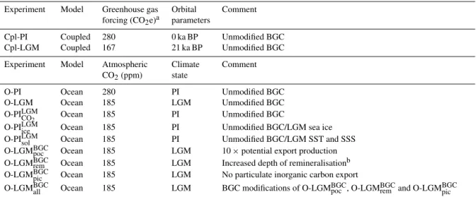
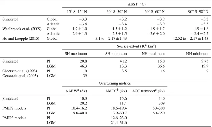
The simulated change in SST between the Cpl-PI and the Cpl-LGM simulations shows a similar magnitude and spatial structure to proxy reconstructions and prior modelling stud-ies, with the greatest cooling in the equatorial oceans, high latitudes and eastern boundary currents and the least cool-ing in the subtropics and western boundary current regions (Fig. 1; Table 2). The global SST mean of the Cpl-LGM was 3.2◦C cooler than the Cpl-PI. This change falls within the range of estimates (∼2–4◦C) produced by other climate models (Alder and Hostetler, 2015; Annan and Hargreaves, 2013; Braconnot et al., 2007) but sits towards the cooler lim-its of previous multiproxy SST reconstructions that estimate a change of 2±1.8◦C (Ballantyne et al., 2005; Waelbroeck et al., 2009). However, a recent reanalysis of the proxy data presented by Waelbroeck et al. (2009) showed past estimates may have underestimated cooling by as much as 50 % (Ho and Laepple, 2015). This finding reconciles some disagree-ment between climate models and palaeoproxies and places our simulated cooling of 3.2◦C well within the bounds of uncertainty in reconstructions.
Table 2.Changes in sea surface temperature (SST), sea ice extent and large-scale circulation between the LGM and PI simulations. SST changes are compared with proxy reconstructions of SST generated by Waelbroeck et al. (2009) and Ho and Laepple (2015), who use different proxies for their reconstructions to produce the differences depicted here and discussed in the text. The values of AABW and NADW formation provided by the models from the Palaeoclimate Modelling Intercomparison Project Phase II (PMIP2) are presented by Otto-Bliesner et al. (2007). The transport rate of the Antarctic Circumpolar Current (ACC) for the PMIP2 models is presented by Lynch-Stieglitz et al. (2016). The estimates of NADW production provided by the PMIP3 models were taken from Muglia and Schmittner (2015).
1SST (◦C)
15◦S–15◦N 30◦S–30◦N 60◦S–60◦N 90◦S–90◦N
Simulated Global −3.3 −3.2 −3.9 −3.2
Atlantic −3.6 −3.4 −3.9 −3.3
Waelbroeck et al. (2009) Global −1.7±1.0 −1.5±1.2 −1.9±1.7 −1.9±1.8 Atlantic −2.9±1.3 −2.3±1.5 −2.6±2.0 −2.4±2.2 Ho and Laepple (2015) Global −5.1 to−2.17±1.43 −12.52 to−2.17±1.43
Sea ice extent (106km2)
SH maximum SH minimum NH maximum NH minimum
Simulated PI 20.8 4.12 15.0 9.73
LGM 46.3 13.3 36.6 19.9
Gloersen et al. (1993) PI 19 3.5 16 9
Gersonde et al. (2005) LGM 39
Overturning metrics
AABWa(Sv) AMOCb(Sv) ACC transportc(Sv)
Simulated PI 10.3 15.6 140
LGM 20.2 11.4 309
PMIP2 models PI 10.4–16.2 18.6–19.4 50–300
LGM 19.6–40.0 13.9–30.7 80–350
PMIP3 models PI 12.6–23.0
LGM 21.4–31.6
aThe rate of Antarctic Bottom Water (AABW) formation is calculated as the annual average of the most negative rate of overturning (Sv) in the Southern Ocean south of
60◦S and deeper than 500 m.bThe rate of overturning in the Atlantic Meridional Overturning Circulation (AMOC) is calculated as the annual average of the most positive
rate of overturning (Sv) in the North Atlantic Ocean north of 0◦and deeper than 500 m.cThe transport of water by the Antarctic Circumpolar Current (ACC) is calculated
as the annual and zonal average of the barotropic stream function at 60◦S.
in excess of 4◦C cooler than the Cpl-PI climate. Meanwhile, the Western Pacific Warm Pool, subtropical gyres and west-ern boundary currents cooled less (0.5–3.0◦C). Again, proxy (Waelbroeck et al., 2009) and climate modelling (Annan and Hargreaves, 2013) are consistent with both the magnitude and spatial pattern of cooling. A notable example of model– data agreement is in the Pacific sector of the Southern Ocean, where SSTs were up to and in excess of 4◦C cooler at the LGM (Benz et al., 2016). Enhanced cooling in the high lat-itudes and in the eastern boundary currents generated strong zonal and meridional temperature gradients relative to Cpl-PI SST. There is a consistent regional pattern to SST cool-ing in the LGM emergcool-ing from proxy and model simulations (Annan and Hargreaves, 2013; Braconnot et al., 2007) that is broadly consistent with our simulated cooling.
Where there is still large uncertainty in SST change at the LGM is in the tropical ocean (see Annan and Hargreaves, 2015, for a review). The Cpl-LGM cooling of 3.3◦C across the tropical ocean (15◦S–15◦N) is greater than other
simula-tions (Annan and Hargreaves, 2013; Braconnot et al., 2007) but falls well within the −5.1 to −2.17◦C estimated by Ho and Laepple (2015). Regionally, climate models (Otto-Bliesner et al., 2009) and proxies (Waelbroeck et al., 2009) agree that cooling in the tropical Atlantic Ocean probably ex-ceeded cooling in the tropical Pacific and Indian oceans by roughly 1◦C. In contrast, the tropical Pacific Ocean cooled by 2◦C more than the tropical Atlantic and Indian oceans in the Cpl-LGM simulation. Although SSTs in the east equato-rial Pacific have been reported as 1.5–3.0◦C cooler than the PI (Dubois et al., 2014; Kucera et al., 2005), the simulated cooling over much of the tropical Pacific appears excessive compared to previous simulations (Braconnot et al., 2007).
3.1.2 Sea ice extent
al-Figure 1.Annual sea surface temperature (SST) difference between (a)the coupled PI experiment, Cpl-PI and the observations from Levitus (2001) and (b)the difference between the coupled LGM and PI experiments (Cpl-LGM−Cpl-PI). Solid contour lines denote positive changes in SST by 4 and 8◦C, while negative changes in SST are denoted by dashed lines at 4 and 8◦C.
though there is evidence that sea ice has declined by 20 % since the 1950s (Curran et al., 2003), the strong agreement between the Cpl-PI sea ice fields and the observations of Glo-ersen et al. (1993) provide a benchmark for assessing LGM sea ice changes.
Associated with cooler SSTs, sea ice coverage (fractional sea ice area≥15 %) was greatly expanded in the Cpl-LGM for both hemispheres relative to the Cpl-PI (Fig. 2, Table 2). In the Southern Hemisphere, total sea ice coverage increased by ∼120 and ∼225 % at its seasonal maximum and min-imum, respectively, relative to the Cpl-PI. In the Northern Hemisphere, total sea ice coverage increased by ∼145 % and∼105 % at its seasonal maximum and minimum, respec-tively, relative to the Cpl-PI. These increases correspond to equatorward expansions of the sea ice field of between 5–
10◦around the Southern Ocean and in excess of 15◦in both the North Atlantic and Pacific oceans.
The simulated expansion of sea ice around much of the Southern Ocean agrees well with proxy reconstructions. Maximum sea ice extent reached as far north as 47◦S in both the Atlantic and Indian sectors (Gersonde et al., 2005) and as far north as 55◦S in the Pacific sector of the Southern Ocean (Benz et al., 2016; Gersonde et al., 2005; Fig. 2). The mag-nitude of growth in the Atlantic and Indian sectors has been tested and largely supported by subsequent studies (Collins et al., 2012; Xiao et al., 2016) and is consistent with our Cpl-LGM sea ice field. In the Pacific sector, however, the simu-lated maximum sea ice edge extends well equatorward of the 55◦S boundary that has been defined by Benz et al. (2016) (Fig. 2). By comparing the coverage of sea ice in the South-ern Hemisphere of the Cpl-LGM (∼46×106km2) with that estimated by Gersonde et al. (2005) (∼39×106km2), we can attribute the simulated excess of sea ice in the glacial Southern Ocean to a possible overestimate in the Pacific sec-tor.
The Cpl-LGM sea ice was broadly consistent with recon-structions in the North Atlantic, with the exception that too much ice covered the Nordic Seas. The central and eastern parts of the subpolar North Atlantic, including the Nordic Seas, are thought to have been at least seasonally ice-free (Pflaumann et al., 2003; De Vernal et al., 2005). The Cpl-LGM sea ice field showed strong, year-round cover in these regions. However, better model–proxy agreement was pro-duced in other parts of the North Atlantic. Perennial sea ice cover was present in the Greenland Sea and Fram Strait dur-ing the LGM (Müller et al., 2009; Telesi´nski et al., 2014). There is also evidence that winter sea ice reached south of Iceland to fill much of the Labrador Sea (Pflaumann et al., 2003) and extended along the eastern Canadian margin (De Vernal et al., 2005). These features were produced in the Cpl-LGM simulation.
Figure 2.Annual average sea ice cover for(a)the Cpl-PI Northern Hemisphere,(b)the Cpl-LGM Northern Hemisphere,(c)the Cpl-PI Southern Hemisphere and(d)the Cpl-LGM Southern Hemisphere. The red and blue contour lines in each projection represent the maximum and minimum seasonal sea ice extents (where sea ice concentration equals 15 % as per Gersonde et al., 2005). In(b), the dashed orange contour line represents the maximum seasonal sea ice extent produced by the Institut Pierre Simon Laplace (IPSL) climate system model, which took part in the PMIP3 LGM experiment, and is broadly consistent with the results of other PMIP3 models. In(d), the coloured markers represent locations were winter sea ice was deemed to have been present (blue) and absent (red) at the LGM according to Gersonde et al. (2005).
3.1.3 Meridional overturning circulation
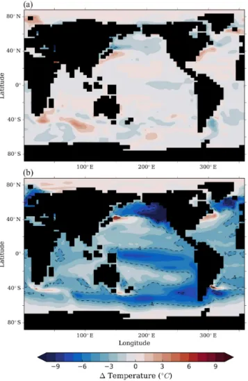
The changes observed in the surface ocean within the Cpl-LGM climate were accompanied by changes in the global meridional overturning circulation (Fig. 3; Table 2). The rate of Antarctic Bottom Water (AABW) formation in the South-ern Ocean doubled between the Cpl-PI and Cpl-LGM ex-periments, increasing from 10.3 to 20.2 Sv. An increase in surface density of 0.9 kg m−3 between 60 to 40◦S drove this intensification and also strengthened transport by the Antarctic Circumpolar Current (ACC) from 140 to 309 Sv. Meanwhile, the Atlantic Meridional Overturning Circulation (AMOC) weakened from 15.6 to 11.4 Sv. The weakened glacial AMOC was also associated with a shoaling of its lower boundary from approximately 3000 to 1500 m. As a
result, much of the Atlantic Ocean below 1500 m was domi-nated by AABW as part of the lower overturning cell.
Figure 3.The upper panels depict the total meridional overturning stream function (Sv) for the global ocean in the(a)Cpl-PI and(b) Cpl-LGM simulations. The bottom panels depict the total meridional overturning stream function (sv) for the Atlantic ocean in the(c)Cpl-PI and(d)Cpl-LGM simulations. Note that those latitudes corresponding to the Southern Ocean are obscured for(c, d)in the Atlantic Ocean, as these overturning velocities are invalid considering that waters can exit to the east and west and that the stream function does not account for these losses.
have linked these changed to the expansion of sea ice in the Southern Ocean, which caused a greater proportion of Cir-cumpolar Deep Water to rise into a zone of negative buoy-ancy flux and thereby produce greater quantities of denser AABW.
However, contradictory changes in the glacial overturning circulation have been simulated in other climate system mod-els. The rates of AABW formation tend to increase under LGM conditions (Otto-Bliesner et al., 2007), but responses of the AMOC among models are highly variable. In earlier experiments as part of the PMIP2 project, the AMOC re-sponse ranged between 40 % above and below the PI rate of overturning (Weber et al., 2007). Our weakened (∼35 %) and shallower (∼50 %) glacial AMOC is therefore consis-tent with the lower bounds of these simulations, as are our rates of AABW formation (Table 2). More recent LGM sim-ulations as part of the PMIP3 project, however, developed stronger and deeper glacial AMOCs (Muglia and Schmit-tner, 2015). Furthermore, a recent reconstruction of South-ern Ocean circulation indicates that extreme intensifications of AABW formation and ACC transport at the LGM are unlikely (Lynch-Stieglitz et al., 2016). Consequently, these results challenge our simulated changes in meridional over-turning, as well as the prevailing interpretation of palaeonu-trient evidence.
Despite inconsistencies between climate model simula-tions, palaeonutrient reconstructions continue to support the
existence of a shallower AMOC overlying southern source waters during glacial periods. Variations in the isotopic sig-nature of Neodynium, for instance, indicate that AABW was more dominant in the deep ocean during the LGM and that its mixing with a glacial form of North Atlantic Deep Water (NADW) was more intense (Howe et al., 2016). These and other authors (Burckel et al., 2016) find further support for the presence of a shallower AMOC above 2500 m. Moreover, simulated distributions of carbon isotopes across a range of idealised circulations have shown that a shallower AMOC is necessary to optimise model–proxy agreement at the LGM (Menviel et al., 2016). Importantly, our Cpl-LGM simula-tion developed an increased presence of AABW throughout the global deep ocean and the development of a shallower AMOC.
3.2 LGM climate: biogeochemical fields
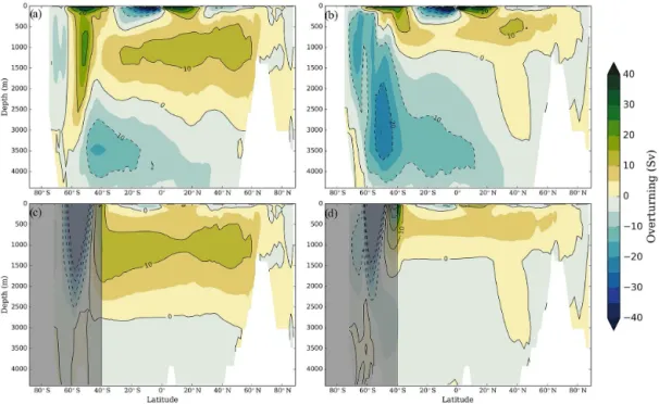
Figure 4.Changes in the concentration of dissolved inorganic carbon (mmol m−3) of the ocean due to physical differences between the pre-industrial (PI) and Last Glacial Maximum (LGM). Panels on the left represent the zonally averaged differences between experiments (a)O-PILGMCO
2 and(b)O-LGM with the O-PI experiment and therefore show total changes in carbon content due to all physical changes associated with the LGM climate. Panels on the right represent the depth-averaged differences between experiments(c)O-PILGMsol and(d) O-PILGMice with the O-PILGMCO
2 experiment and therefore represent the contribution of solubility and sea ice changes at the LGM to carbon storage in the ocean.
3.2.1 Carbon
For experiment O-LGM, the dissolved inorganic carbon (hereafter referred to as carbon) content of the ocean was 622 Pg C less than in the O-PI experiment (Fig. 4; Table 3). The net loss of carbon reflected the combined effect of phys-ical changes to the ocean, which include an increase in sol-ubility due to cooling, an expanded sea ice field, an al-tered overturning circulation and the tendency for outgassing caused by a lower pCO2. The physical changes were suffi-cient in combination to increase carbon in the deep ocean by 267 Pg C. However, lowering the atmospheric pCO2 to 185 ppm drove a large amount of carbon out of the ocean, causing a loss of 889 Pg C from waters in the upper 2000 m. The combined effect of our simulated LGM physical state could therefore not overcome the equilibration with a lower atmosphericpCO2concentration.
The increase in carbon content in the glacial deep ocean did suggest that despite the net loss caused by outgassing, the glacial ocean was indeed conducive to storing carbon. The loss of carbon from the ocean of experiment O-PILGMCO 2
demonstrated this (Fig. 4; Table 3). The ocean carbon con-tent of O-PILGMCO
2 evolved to be 1290 Pg less than in the O-PI experiment, which placed the O-LGM carbon content as 668 Pg greater than O-PILGMCO
2 . This confirmed that the glacial ocean had a greater ability to store carbon than the PI ocean. To investigate this further, the individual contributions of glacial solubility, sea ice and circulation to carbon seques-tration were determined by comparing the idealised exper-iments of O-PILGMice and O-PILGMsol to O-PILGMCO
T ab le 3. Global ocean av eraged diagnostics from the model simulations described in T able 1. The subscript or g anic refers to the in v entory due to the remineralisation computed from the apparent oxygen utilisation. POC and PIC refer to the annual export of particulate or g anic and inor g anic carbon from the upper 50 m, respecti v ely . The tracer columns refer to global ocean in v entory or global ocean mean v alues. Global in v entory of phosphate w as 2.68 Pmol in all simulations. Model Atmospheric a POC PIC 1 Carbon b C or g Oxygen (mean) Depth c (m) CO 2 (ppm) (Pg C year − 1 ) (Pg C year − 1 ) (Pg C) (Pg C) (mmol m − 3 ) where ca = 1 Global Southern Ocean d Global Global Upper e Deep f Global Upper e Deep f O-PI 280 8.02 1.60 0.64 0g 0 g 0 g 1650 181 182 180 2666 O-PI LGM CO 2 185 8.02 1.60 0.64 − 1290 − 692 − 598 1650 181 182 180 3234 O-PI LGM sol 185 8.02 1.60 0.64 − 941 − 435 − 346 1361 206 195 217 3222 O-PI LGM ice 185 7.96 1.44 0.64 − 1450 − 759 − 691 1676 179 181 177 3233 O-LGM 185 4.48 0.76 0.36 − 622 − 889 + 267 665 280 262 300 3208 O-LGM BGC poc 185 5.96 4.06 0.47 − 443 − 981 + 537 772 271 270 272 3297 O-LGM BGC rem 185 3.25 0.75 0.26 − 455 − 790 + 335 720 275 265 287 3254 O-LGM BGC pic 185 4.48 0.76 0.00 − 293 − 451 + 158 665 280 262 300 3196 O-LGM BGC all 185 4.86 3.43 0.00 + 317 − 419 + 737 1004 251 264 237 2839 a Atmospheric CO 2 is prescribed in each experiment. b Change in the ocean in v entory of carbon relati v e to experiment O-PI with atmospheric p CO 2 at 280 ppm. c Where the calcite saturati on horizon ( ca = 1 ) exceeds the depth of the ocean, the lo wer depth bound of the deepest grid box w as included in the av eraging process. d All grid box es south of 45 ◦ S. e All grid box es abo v e 2000 m depth. f All grid box es belo w 2000 m depth. g Steady-state carbon content of the global, upper and deep ocean under pre-industrial conditions is 34 114, 17 458 and 16 656 Pg C, respecti v ely .
carbon in O-LGM. The isolated effect of the glacial circu-lation was the addition of 479 Pg C, which was calculated by solving for the difference between the combined effect of solubility and sea ice (189 Pg C) and the gain between the O-LGM and O-PILGMCO
2 experiments (668 Pg C).
Therefore, we primarily implicate circulation and secon-darily solubility changes as the physical drivers of oceanic carbon storage at the LGM, while presenting sea ice expan-sion as a mechanism for reducing ocean carbon storage. Re-garding solubility, previous work has constrained the effect of glacial solubility on atmospheric carbon to approximately 15 ppm (Kohfeld and Ridgwell, 2009; Sigman and Boyle, 2000). By taking the 1290 Pg C difference between the O-PI and O-PILGMCO2 experiments and assuming an a priori addition of 520 Pg C in a glacial ocean (Ciais et al., 2011), we can attribute approximately 18 ppm to our simulated solubility changes (Table 4). Our results are therefore roughly consis-tent with other estimates. The tendency for carbon to be re-leased to the atmosphere would have been further reduced by storing more carbon in the deep ocean. We therefore note that circulation changes and cooling would have had a comple-mentary effect on carbon sequestration and magnified their individual effects.
Regarding sea ice, a prevailing view is that sea ice expan-sion would enhance oceanic carbon storage by limiting air– sea gas exchange (Stephens and Keeling, 2000). This theory largely focuses on the restriction of outgassing from carbon-rich deep waters that upwell in the Southern Ocean. How-ever, this neglects responses in the Northern Hemisphere and in the biological pump. In a seminal paper, Marinov et al. (2006) showed that export production and circulation in the Antarctic zone have a strong effect on atmospheric CO2. We found that light limitation of highly productive regions in both hemispheres caused by increased sea ice cover led to a global loss of 160 Pg C, equivalent to 8 ppmpCO2. Simi-lar responses have been simulated in other models that con-sider the impact of sea ice on biological production and do not consider temperature and salinity changes associ-ated with sea ice growth (Kurahashi-Nakamura et al., 2007; Sun and Matsumoto, 2010).
Our results demonstrated that although the storage of car-bon was enhanced in the glacial ocean (668 Pg C) due to physical changes, namely due to the overturning circula-tion, they could not overcome the loss of carbon (1290 Pg C) caused by equilibration with a lower atmosphericpCO2.
3.2.2 Nutrients and export production
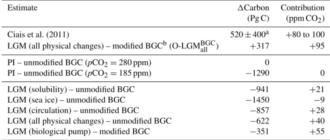
Table 4.A summary of the total changes in ocean carbon storage and their drivers between our simulated pre-industrial (PI) and Last Glacial Maximum (LGM) climates. We use the increase in carbon of our O-LGMBGCall experiment of 317 Pg C, which falls within the estimate range of ocean carbon storage at the LGM (Ciais et al., 2011), and our simulated loss of 1290 Pg C from the PI ocean with an atmosphericpCO2 of 185 ppm to determine the contribution of physical and biogeochemical drivers in ppm of CO2. For example, an addition of 1607 Pg C in excess of experiment O-PILGMCO
2 (+317 Pg C in column 2) would constitute a contribution of 95 ppm. BGC refers to biogeochemistry.
Estimate 1Carbon Contribution
(Pg C) (ppm CO2)
Ciais et al. (2011) 520±400a +80 to 100
LGM (all physical changes) – modified BGCb(O-LGMBGCall ) +317 +95
PI – unmodified BGC (pCO2=280 ppm) 0
PI – unmodified BGC (pCO2=185 ppm) −1290 0
LGM (solubility) – unmodified BGC −941 +21
LGM (sea ice) – unmodified BGC −1450 −9
LGM (circulation) – unmodified BGC −857 +28 LGM (all physical changes) – unmodified BGC −622 +40 LGM (biological pump) – modified BGC −351 +55
aEstimate of increase in ocean carbon content during the LGM made by Ciais et al. (2011), whereby atmospheric carbon
was reduced by 194±2 Pg C and terrestrial carbon was reduced by 330±400 Pg C.bAssumes all three biological
modifications that were postulated (see Table 1, experiments O-LGMBGCpoc , O-LGMBGCrem and O-LGMBGCpic ) occurred to
provide an upper bound estimate of ocean carbon storage.
(Boyle, 1992; Gebbie, 2014; Marchitto and Broecker, 2006; Tagliabue et al., 2009).
A direct consequence of the redistribution of PO4 was the reduction in the production of particulate organic mat-ter across many regions of the O-LGM ocean (Fig. 5). With the exception of the South Pacific and isolated areas in the subtropics, export production in the O-LGM experiment de-creased relative to the O-PI experiment, so that global ex-port production was 56 % of O-PI. The global reduction was also illustrated by a decrease in regenerated carbon (Corg), which indicated that the biological carbon pump was weak-ened (Table 3). The reduction in export production and re-generated carbon for the O-LGM experiment is significant when compared with other studies that argue for a more effi-cient glacial biological pump than that of the Holocene (Gal-braith and Jaccard, 2015; Schmittner and Somes, 2016). The weakened efficiency of our simulated biological pump can be attributed, in part, to a large decrease in export produc-tion from the subantarctic zone. This feature is in direct con-flict with palaeoproductivity proxies in the Atlantic and In-dian sectors of the subantarctic Ocean (Anderson et al., 2002, 2014; Chase et al., 2001; Jaccard et al., 2013; Nürnberg et al., 1997) and some parts of the Pacific sector (Bradtmiller et al., 2009; Lamy et al., 2014). Outside of the Southern Ocean, the reduction in export production in the O-LGM experiment is largely consistent with palaeoproductivity evidence (see In-troduction).
3.2.3 Carbonate chemistry
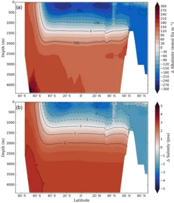
The loss of phosphate from the upper ocean and its in-crease at depth was mirrored by changes in alkalinity and
salinity, so that a more alkaline and saline signature of AABW, relative to NADW, dominated the deep ocean in experiment O-LGM. Alkalinity and salinity decreased by 66 mmol Eq m−3and 0.37 PSU in the surface ocean and in-creased by 147 mmol Eq m−3and 2.71 PSU in the deep ocean (Fig. 6).
Because the majority of LGM–PI change in salinity oc-curred in the deep ocean, the changes in carbonate chem-istry across the surface ocean were small. Little change be-tween experiments O-PI and O-LGM was found in the arag-onite saturation state (ar), which is a unitless index indicat-ing under- and super-saturation at values below and above 1 (Fig. 7). Surfacearbetween 40◦S and 40◦N in O-LGM (ar=3.8) was slightly lower than that of O-PI (ar=4.0) but increased in the high-latitude oceans. Consequently, the simulated ar=3.25 isoline, the value at present used to define the location of viable coral reef conditions (Hoegh-Guldberg et al., 2007), was nearly unchanged between the O-LGM and O-PI experiments. Recent sonar and coring in the southern portion of the Great Barrier Reef (Abbey et al., 2011; Yokoyama et al., 2011) have detected the presence of drowned coral reefs that existed at the LGM as far south as reefs present today. Such observations are consistent with our O-LGM experiment and indicates that the extent of viable coral reefs was unlikely to have been significantly different at the LGM relative to today.
Figure 5.Changes in the export production of particulate organic matter (POC) and Phosphate concentrations between the O-LGM and O-PI experiments.(a)Annually averaged export of POC from the upper 50 m (g C m−2year−1) for O-PI,(b)the O-LGM−O-PI difference in Phosphate concentrations (mmol m−3) and(c)the O-LGM−O-PI difference in export production of POC from the upper 50 m (g C m−2year−1).
from 2666 m in O-PI to 3208 m in O-LGM. While this in-crease may seem modest, the inin-crease exceeded the ocean floor over the majority of the ocean, so that seawater was completely saturated for calcite outside of the eastern tropical Pacific (Fig. 8). There is strong evidence that the carbonate chemistry of the LGM ocean was not appreciably different to the late Holocene (Yu et al., 2014), and this information places our simulated changes in deep-oceancaat the LGM as unrealistic.
Figure 6. Change in the zonally averaged global distribution of (a)alkalinity (mmol Eq m−3) and(b)salinity (PSU) between the O-LGM and O-PI experiments (O-O-LGM−O-PI). Despite the strong re-duction in salinity in the upper ocean of the O-LGM experiment rel-ative to O-PI, the whole-ocean salt content was greater by 1.0 PSU.
3.2.4 Dissolved oxygen
Figure 7. The annual average surface aragonite saturation state (ar) calculated from(a) the observations of Key et al. (2004),
(b)the O-PI experiment and(c)the O-LGM experiment.
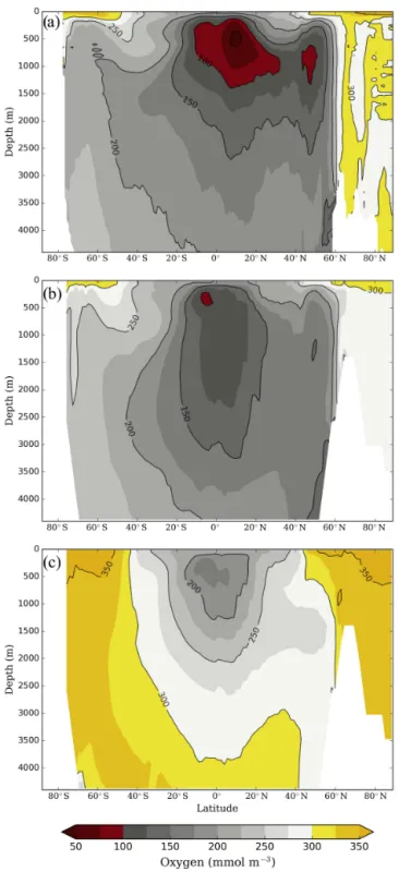
Figure 9. Zonally averaged dissolved oxygen concentrations (mmol m−3) in(a)the modern ocean according to the World Ocean Atlas (Garcia et al., 2013),(b)the O-PI experiment and(c)the O-LGM experiment.
water column denitrification rates over the past 200 000 years were lower during glacial periods and higher during inter-glacial periods (Galbraith et al., 2004), and this is consistent with the simulated oxygenation of the upper ocean.
However, dissolved oxygen concentrations in the deep ocean increased to an average of 300 mmol O2m−3 in O-LGM, and this contrasts starkly with existing palaeoclimate reconstructions. Deep waters of the Indian Ocean (Murgese et al., 2008; Sarkar et al., 1993; Schmiedl and Mackensen, 2006), North Atlantic (Hoogakker et al., 2014), Southern Ocean (Chase et al., 2001; Jaccard et al., 2016) and equa-torial Pacific (de la Fuente et al., 2015) were poorly ven-tilated at the LGM relative to the Holocene. Drawing on a global compilation of similar studies, Jaccard and Galbraith (2012) and Jaccard et al. (2014) demonstrated that the deep ocean was largely deoxygenated relative to the Holocene on a global scale. While the increase in oxygen concentrations in the upper ocean aligned with the direction of change in-ferred from proxies, the response in the deep ocean can be considered unrealistic.
3.3 Importance of ocean biogeochemistry for climate
The carbon content, export production field, carbonate chem-istry and deep-ocean oxygen content of experiment O-LGM are outstanding in their disagreement with proxy evidence. Notably, 622 Pg C was lost from experiment O-LGM relative to O-PI. The standard LGM simulation was therefore unable to explain the glacial–interglacial drawdown of atmospheric CO2, despite the existence of a physical ocean state within realistic bounds. If we are to reconcile the biogeochemistry of the glacial ocean with that inferred from proxy evidence, we must therefore consider altering ocean biogeochemistry.
3.3.1 Reconciling the carbon budget
Three plausible modifications to ocean biogeochemistry (see methods) were considered: (1) increased POC export produc-tion, (2) increased depth of POC remineralisation and (3) reduced PIC export. In the following we step through the changes to carbon content caused by each modification, and the reader is directed to Table 3 for reference.
lower than the O-PI experiment of 8.02 Pg C year−1, this increased carbon content by 179 Pg C.
2. Experiment O-LGMBGCrem . The shift of organic matter to depth was associated with a global reduction in POC export production of∼1.2 Pg C year−1as remineralisa-tion released PO4 and carbon further from the photic zone. Despite the reduction in the biological pump, the bulk transfer of POC to depth generated an increase in ocean carbon storage of 167 Pg C.
3. Experiment O-LGMBGCpic . The elimination of PIC in the simulated glacial ocean increased the solubility of CO2 in the surface ocean and enabled the ocean to store an additional 329 Pg C.
Independently, none of the above modifications were able to increase ocean carbon content relative to the O-PI experi-ment (O-LGMBGCpoc :−443 Pg C; O-LGMBGCrem :−455 Pg C; O-LGMBGCpic :−293 Pg C). However, by employing all three bio-geochemical modifications in one experiment (experiment O-LGMBGCall ), the glacial ocean was able to store an addi-tional 939 Pg C more than experiment O-LGM and 317 Pg C more than O-PI.
This magnitude of increase places our glacial ocean state within the plausible bounds required to offset the loss of atmospheric and terrestrial carbon reported by Ciais et al. (2011) of ∼520±400 Pg C at the LGM (Table 4). By as-suming a glacial–interglacial difference in atmospheric CO2 of 95 ppm and applying this to our changes in carbon con-tent, we attribute roughly 40 ppm to changes in ocean physics and 55 ppm to changes in the biological pump. Within the physical changes, 28 ppm is attributed to the reorganisation of the global overturning circulation, while 12 ppm can be attributed to changes in surface properties, including sea ice expansion, cooling and salinification.
3.3.2 Reconciling export production
Of the three biogeochemical modifications applied to the LGM ocean, only two had an effect on POC export, as the amount of PIC exported from the photic zone has no influ-ence on the amount of POC export. Deepening the remineral-isation of POC (O-LGMBGCrem ) shifted a greater fraction of re-generated PO4into the deep ocean, which resulted in a global reduction of export production. Increasing the scaling factor (O-LGMBGCpoc ), however, caused an increase in global export production from 4.48 to 5.96 Pg C year−1. Most of this in-crease occurred in the Southern Ocean, particularly the sub-antarctic zone, and in a few isolated pockets in the northwest Pacific and North Atlantic where excess nutrients were avail-able (Fig. 10).
The increase in the scaling factor dominated the change in export production produced when combining all three biogeochemical modifications (O-LGMBGCall ). The strong in-crease in export production observed in the subantarctic was
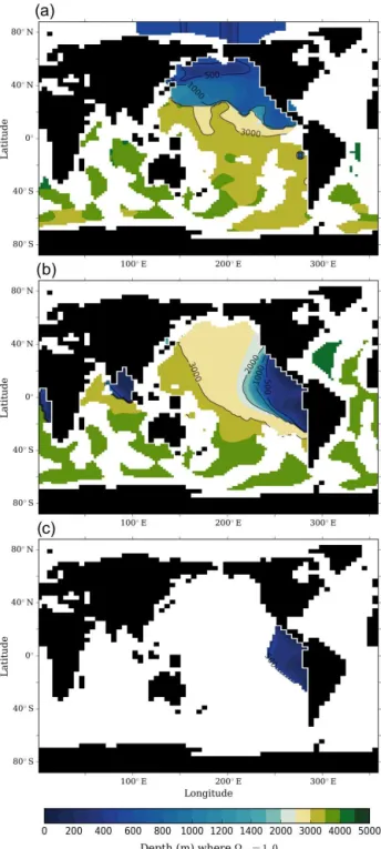
Figure 11.The depth at which calcite becomes undersaturated in the water column (whereca=1) for the experiments with modified biogeochemical formulations.(a)O-LGMBGCpoc ,(b)O-LGMBGCrem ,(c)O-LGMBGCpic and(d)O-LGMBGCall . The white areas in the ocean are regions where calcite is completely saturated throughout the water column.
clearly replicated within this experiment and reconciles our simulated export production field with current evidence of productivity at the LGM. In the Southern Ocean, the Atlantic and Indian sectors of the subantarctic zone experienced a greater flux of organics (Anderson et al., 2002, 2014; Chase et al., 2001; Jaccard et al., 2013; Nürnberg et al., 1997). Whether this was also the case for the Pacific sector remains under debate, with some evidence for increase (Bradtmiller et al., 2009; Lamy et al., 2014) and some for no change (Bo-stock et al., 2013; Chase et al., 2003). Meanwhile, it is widely accepted that waters south of the Antarctic Polar Front were reduced in their productivity (Bostock et al., 2013; Chase et al., 2003; Elderfield and Rickaby, 2000; Francois et al., 1997; Frank et al., 2000; Kohfeld et al., 2005; Kumar et al., 1995; Mortlock et al., 1991; Ninnemann and Charles, 1997; Shemesh et al., 1993), likely due to increased sea ice extent (Benz et al., 2016; Gersonde et al., 2005; Jaccard et al., 2013) and stratification (Anderson et al., 2014; Jaccard et al., 2005). In experiment O-LGMBGCall , net export production re-mained less than the in O-PI experiment by 3.16 Pg C year−1 despite the application of biogeochemical modifications. The weakened carbon transfer to the interior ocean was also ob-served in the regenerated carbon content of the ocean (Corg), which was 646 Pg less than in the O-PI experiment (Ta-ble 3). The net decline in export production observed in this study was dominated by the decline in tropical and sub-tropical waters. Many palaeoproductivity studies located out-side of the subantarctic zone have found weakened
produc-tivity at the LGM (Chang et al., 2014, 2015; Costa et al., 2016; Crusius et al., 2004; Kohfeld et al., 2005; Kohfeld and Chase, 2011; Jaccard et al., 2005; McKay et al., 2015; Or-tiz et al., 2004; Riethdorf et al., 2013; Salvatteci et al., 2016; Singh et al., 2011; Thomas et al., 1995). Additionally, an en-hanced utilisation of available nutrients in the subantarctic zone (Martinez-Garcia et al., 2014) would reduce the nu-trient content of intermediate waters formed in the South-ern Ocean and would thus reduce the delivery of nutrients to lower latitudes (Sarmiento et al., 2004). This mechanism coupled with cooler temperatures caused reductions in ex-port production across much of the mid- and lower-latitude oceans in experiment O-LGMBGCall , which maintains the qual-itative agreement between the simulated export production field and proxy observations. However, the global weaken-ing of the biological pump in our simulations is contrary to proxy and model-based evidence for a strengthened biologi-cal pump (>Corg) at the LGM (Galbraith and Jaccard, 2015; Schmittner and Somes, 2016). Hence, while we present im-proved spatial agreement between O-LGMBGCall and palaeo-productivity proxies at the LGM, which was essential to in-creasing the carbon content of the ocean, we note that addi-tional increases in the export production field may be valid.
3.3.3 Reconciling carbonate chemistry
Figure 12.Change in oxygen concentration (mmol m−3) at 500 m between the LGM and PI for the experiments with modified biogeochem-ical formulations.(a)O-LGMBGCpoc −O-PI,(b)O-LGMBGCrem −O-PI,(c)O-LGMBGCpic −O-PI and(d)O-LGMBGCall −O-PI. A depth of 500 m is representative of the depth at which the greatest extent of low-oxygen water exists in the simulated PI climate. It should be noted that the oxygen field for experiment O-LGMBGCpic , whereby particulate inorganic carbon was set to zero, did not differ from the unmodified glacial experiment O-LGM and can therefore be used here as a reference to that simulation.
saturated for calcite in the O-LGM experiment, additional processes were required to shoal the depth at which calcite becomes unsaturated (ca=1) and thereby reconcile proxy evidence.
One mechanism to reduce deep-oceancawould be to re-duce continental inputs of alkalinity at the LGM. However, the presence of glaciers, drier atmospheric conditions and the exposure of continental shelves due to lower sea level would have increased the supply of carbonates to the ocean (Gibbs and Kump, 1994; Riebe et al., 2004), thereby increas-ing ocean alkalinity and further deepenincreas-ing the carbonate sat-uration horizon. This mechanism has been largely refuted as having a significant effect on the glacial–interglacial differ-ence in the carbon budget (Brovkin et al., 2007; Foster and Vance, 2006; Jones et al., 2002) and can therefore be ignored. The individual biogeochemical modifications were also in-sufficient to reduce ca to be consistent with palaeo evi-dence. However, combining all three modifications in exper-iment O-LGMBGCall reduced ca significantly (Fig. 11) and produced a globally averaged calcite saturation horizon at 2839 m. Remarkably, our simulated PI to LGM changes in ca are also consistent with palaeoproxy reconstructions in a regional sense. The calcite saturation horizon in the Pacific Ocean was deeper in experiment O-LGMBGCall relative to O-PI but was shallower in the Atlantic Ocean and within the Atlantic and Indian sectors of the subantarctic zone. Similar changes are seen in the proxy record, with a deepening of
less than 1000 m in the North Pacific and Southern Ocean at the LGM (Anderson et al., 2002; Catubig et al., 1998) and a shoaling in the Atlantic Ocean (Anderson et al., 2002).
An important caveat of this study, which cannot be ig-nored, is the exclusion of calcium carbonate (CaCO3) burial within ocean sediments. Because this process is not included in the model, it is highly likely that the deepening of the cal-cite saturation horizon that occurred in the standard LGM experiment (O-LGM) was too extreme. CaCO3burial lowers the alkalinity of the glacial ocean and is therefore a nega-tive feedback mechanism that modulates changes in carbon-ate chemistry (see Sigman et al., 2010, for a review). If cal-cite saturation increases through the water column, as found in O-LGM, the burial of CaCO3would increase and subse-quently mitigate the rise in whole-ocean alkalinity, which in turn would reduce calcite saturation and the ability of the ocean to store carbon. By not taking this process into ac-count, both the deepening of the calcite saturation horizon and the storage of carbon were overestimated in experiment O-LGM.
Figure 13.Change in oxygen concentration (mmol m−3) at 3500 m between the LGM and PI for the experiments with modified biogeo-chemical formulations.(a)O-LGMBGCpoc −O-PI,(b)O-LGMBGCrem −O-PI,(c)O-LGMBGCpic −O-PI and(d)O-LGMBGCall −O-PI. A depth of
3500 m is representative of the deep ocean. It should be noted that the oxygen field for experiment O-LGMBGCpic , whereby particulate inor-ganic carbon was set to zero, did not differ from the unmodified glacial experiment O-LGM and can therefore be used here as a reference to that simulation.
exaggerated, just as the deepening observed in experiment O-LGM was exaggerated. Again, this can be applied to changes in the carbon content of the ocean, as a shallower calcite sat-uration horizon would have reduced CaCO3burial, thereby increasing whole-ocean alkalinity and the ocean’s ability to take up carbon. This effect would have been particularly im-portant for experiment O-LGMBGCpic , where inorganic carbon export was eliminated. If whole-ocean alkalinity was able to respond to a decrease in CaCO3rain, this would have am-plified the carbon sequestration of experiment O-LGMBGCpic . Therefore, the exclusion of CaCO3 burial in experiment O-LGMBGCall (O-LGM) caused an exaggerated shoaling (deep-ening) of the calcite saturation horizon and an underesti-mated (overestiunderesti-mated) carbon content.
3.3.4 Reconciling dissolved oxygen
As discussed previously, the increase in oxygen concen-trations of the upper ocean in experiment O-LGM is con-sistent with the current assemblage of proxy evidence. All experiments with modified biogeochemistry, including O-LGMBGCall , had little effect on the upper-ocean oxygen con-centration (Fig. 12; Table 3) and therefore did not compro-mise the agreement between simulated and proxy oxygen re-constructions.
Modifying ocean biogeochemistry did, however, have a large effect on the oxygen concentrations of the deep ocean
(Fig. 13). Increasing export production (O-LGMBGCpoc ) and deepening the remineralisation depth (O-LGMBGCrem ) both reduced oxygen concentrations by 28 and 13 mmol m−3, respectively. The combination of these modifications (O-LGMBGCall ) amplified their individual effects, so that deep-ocean oxygen was reduced by 63 mmol m−3relative to O-LGM. The increased sensitivity of deep-ocean oxygen to the combination of increased export production and a deeper remineralisation depth was also observed in the increase in the quantity of regenerated nutrients (Corg) that resulted (Ta-ble 3). A greater proportion of regenerated nutrients relative to preformed nutrients at the LGM has been identified as a key driver of interior ocean deoxygenation (Jaccard and Gal-braith, 2012; Sigman et al., 2010), and this process was cap-tured in experiment O-LGMBGCall .
slower formation rates of major ocean deep waters (as per Menviel et al., 2016) combined with an intensified coverage of sea ice in the region of their formation. The growth of sea ice and the formation rate of AABW were likely too strong in our LGM simulation (see Sects. 3.1.2 and 3.1.3), and we therefore suggest that a sluggish circulation is necessary for reducing deep-ocean oxygen. Key biogeochemical mecha-nisms include a further increase in global export produc-tion, and/or a different spatial pattern of export producproduc-tion, and/or increasing the injection of organic matter to deep wa-ter via further lengthening the remineralisation profile. The weakened biological pump in our LGM simulations contrasts with other studies (Galbraith and Jaccard, 2015; Schmittner and Somes, 2016) and indicates that export production may be underestimated by our simulations. The combination of a more sluggish deep-ocean circulation with an enhanced ex-port of organics would significantly reduce the oxygen con-tent of the deep ocean, while pocon-tentially further increasing carbon storage.
4 Conclusions
In this study we have shown that simulated physical changes in the ocean state during the climate of the Last Glacial Max-imum are not sufficient to explain the 80–100 ppm draw-down of atmospheric CO2. Physical changes associated with the glacial climate, including an expanded sea ice field, in-creased solubility and a reorganisation of the global overturn-ing circulation, were responsible for roughly 40 ppm of CO2 drawdown. The effect of circulation on carbon storage was greatest at 28 ppm and was associated with an expansion of southern source waters throughout the deep ocean. Thus, var-ious biogeochemical modifications were necessary to fully explain the atmospheric drawdown of CO2during the glacial period. The biogeochemical modifications explored in this study were (1) an increase in export production consistent with greater iron fertilisation, (2) a shift of remineralisation to the deep ocean consistent with cooler temperatures, and (3) a decrease in the production of particulate inorganic car-bon consistent with cooler temperatures and increased de-livery of silicate to lower latitudes. Together, these modifi-cations increased the carbon content of the ocean and, com-bined with physical changes, were able to account for the loss of carbon from the atmosphere and land at the Last Glacial Maximum. Furthermore, their addition improved model– proxy agreement in the fields of export production, carbon-ate chemistry and dissolved oxygen. This study demonstrcarbon-ates that fundamental changes to ocean biogeochemical function are required to explain glacial–interglacial cycles.
5 Data availability
The model output produced during the experiments of this study is held by the Australian National Computational
In-frastructure (NCI) data portal and is available for download at doi:10.4225/41/5859eeac6b473 (Buchanan, 2016).
Acknowledgements. We wish to thank Katsumi Matsumoto and Andreas Schmittner for their reviews that significantly improved the manuscript. Funding for this work was provided by the Australian Climate Change Science Program and CSIRO Wealth from Ocean Flagship. An award under the Merit Allocation Scheme on the NCI National Facility at the Australian National University ensured that numerical simulations could be undertaken. This research was also supported under the Australian Research Council’s Special Research Initiative for the Antarctic Gateway Partnership (Project ID SR140300001). The authors wish to acknowledge the use of the Ferret program (http://ferret.pmel.noaa.gov/Ferret/) for the analysis undertaken in this work. The matplotlib package (Hunter, 2007), Iris and Cartopy packages (http://scitools.org.uk/), and cmocean package (Thyng et al., 2016) were all used for producing visualisations.
Edited by: A. Winguth
Reviewed by: K. Matsumoto and A. Schmittner
References
Abbey, E., Webster, J. M., and Beaman, R. J.: Geomorphology of submerged reefs on the shelf edge of the Great Barrier Reef: The influence of oscillating Pleistocene sea-levels, Mar. Geol., 288, 61–78, doi:10.1016/j.margeo.2011.08.006, 2011.
Adkins, J. F.: The role of deep ocean circulation in set-ting glacial climates, Paleoceanography, 28, 539–561, doi:10.1002/palo.20046, 2013.
Alder, J. R. and Hostetler, S. W.: Global climate simulations at 3000-year intervals for the last 21 000 years with the GEN-MOM coupled atmosphere–ocean model, Clim. Past, 11, 449– 471, doi:10.5194/cp-11-449-2015, 2015.
Anderson, R. F., Chase, Z., Fleisher, M. Q., and Sachs, J.: The Southern Ocean’s biological pump during the Last Glacial Max-imum, Deep-Sea Res. Pt. II, 49, 1909–1938, 2002.
Anderson, R. F., Barker, S., Fleisher, M., Gersonde, R., Goldstein, S. L., Kuhn, G., Mortyn, P. G., Pahnke, K., and Sachs, J. P.: Bi-ological response to millennial variability of dust and nutrient supply in the Subantarctic South Atlantic Ocean, Philos. T. R. Soc. A, 372, 20130054, doi:10.1098/rsta.2013.0054, 2014. Annan, J. and Hargreaves, J.: A perspective on model-data surface
temperature comparison at the Last Glacial Maximum, Quater-nary Sci. Rev., 107, 1–10, doi:10.1016/j.quascirev.2014.09.019, 2015.
Annan, J. D. and Hargreaves, J. C.: A new global reconstruction of temperature changes at the Last Glacial Maximum, Clim. Past, 9, 367–376, doi:10.5194/cp-9-367-2013, 2013.
Archer, D. and Maier-Reimer, E.: Effect of deep-sea sedimentary calcite preservation on atmospheric CO2concentration, Nature, 367, 260–263, doi:10.1038/367260a0, 1994.
Archer, D., Winguth, A., Lea, D., and Mahowald, N.: What caused the glacial/interglacial atmospheric pCO2 cycles?, Rev. Geo-phys., 38, 159–189, doi:10.1029/1999RG000066, 2000. Ballantyne, A. P., Lavine, M., Crowley, T. J., Liu, J., and Baker,
the Last Glacial Maximum, Geophys. Res. Lett., 32, 1–4, doi:10.1029/2004GL021217, 2005.
Benz, V., Esper, O., Gersonde, R., Lamy, F., and Tiedemann, R.: Last Glacial Maximum sea surface temperature and sea-ice ex-tent in the Pacific sector of the Southern Ocean, Quaternary Sci. Rev., 146, 216–237, doi:10.1016/j.quascirev.2016.06.006, 2016. Bostock, H. C., Barrows, T. T., Carter, L., Chase, Z., Cortese, G., Dunbar, G. B., Ellwood, M., Hayward, B., Howard, W., Neil, H. L., Noble, T. L., Mackintosh, A., Moss, P. T., Moy, A. D., White, D., Williams, M. J. M., and Armand, L. K.: A review of the Australian-New Zealand sector of the Southern Ocean over the last 30 ka (Aus-INTIMATE project), Quaternary Sci. Rev., 74, 35–57, doi:10.1016/j.quascirev.2012.07.018, 2013.
Boyle, E. A.: Cadmium and 113C Paleochemical Ocean Distributions During the Stage 2 Glacial Maxi-mum, Annu. Rev. Earth Planet. Sc., 20, 245–287, doi:10.1146/annurev.ea.20.050192.001333, 1992.
Braconnot, P., Otto-Bliesner, B., Harrison, S., Joussaume, S., Pe-terchmitt, J.-Y., Abe-Ouchi, A., Crucifix, M., Driesschaert, E., Fichefet, Th., Hewitt, C. D., Kageyama, M., Kitoh, A., Laîné, A., Loutre, M.-F., Marti, O., Merkel, U., Ramstein, G., Valdes, P., Weber, S. L., Yu, Y., and Zhao, Y.: Results of PMIP2 coupled simulations of the Mid-Holocene and Last Glacial Maximum – Part 1: experiments and large-scale features, Clim. Past, 3, 261– 277, doi:10.5194/cp-3-261-2007, 2007.
Bradtmiller, L. I., Anderson, R. F., Fleisher, M. Q., and Burckle, L. H.: Comparing glacial and Holocene opal fluxes in the Pa-cific sector of the Southern Ocean, Paleoceanography, 24, 1–20, doi:10.1029/2008PA001693, 2009.
Broecker, W. S.: Glacial to interglacial changes in ocean chem-istry, Progress in Oceanography, 11, 151–197, doi:10.1016/0079-6611(82)90007-6, 1982.
Broecker, W. S. and Henderson, G. M.: The sequence of events surrounding termination II and their implications for the causes of glacial interglacial CO2changes, Paleoceanography, 13, 352– 364, 1998.
Brovkin, V., Ganopolski, A., Archer, D., and Rahmstorf, S.: Lower-ing of glacial atmospheric CO2in response to changes in oceanic circulation and marine biogeochemistry, Paleoceanography, 22, PA4202, doi:10.1029/2006PA001380, 2007.
Burckel, P., Waelbroeck, C., Luo, Y., Roche, D. M., Pichat, S., Jac-card, S. L., Gherardi, J., Govin, A., Lippold, J., and Thil, F.: Changes in the geometry and strength of the Atlantic meridional overturning circulation during the last glacial (20–50 ka), Clim. Past, 12, 2061–2075, doi:10.5194/cp-12-2061-2016, 2016. Buchanan, P.: Simulations of glacial climate and
ocean biogeochemistry with the CSIRO Mk3L v1.0, doi:10.4225/41/5859eeac6b473, 2016.
Cannariato, K. G. and Kennett, J. P.: Climatically related millennial-scale fluctuations in strength of California margin oxygen-minimum zone during the past 60 k.y., Geology, 27, 975–978, doi:10.1130/0091-7613(1999)027<0975:CRMSFI>2.3.CO;2, 1999.
Cartapanis, O., Tachikawa, K., and Bard, E.: Northeastern Pacific oxygen minimum zone variability over the past 70 kyr: Impact of biological production and oceanic ventilation, Paleoceanogra-phy, 26, PA4208, doi:10.1029/2011PA002126, 2011.
Catubig, N. R., Archer, D. E., Francois, R., DeMenocal, P., Howard, W., and Yu, E.-F.: Global deep-sea burial rate of calcium
car-bonate during the Last Glacial Maximum, Paleoceanography, 13, 298–310, doi:10.1029/98PA00609, 1998.
Chang, A. S., Pedersen, T. F., and Hendy, I. L.: Effects of pro-ductivity, glaciation, and ventilation on late Quaternary sedimen-tary redox and trace element accumulation on the Vancouver Is-land margin, western Canada, Paleoceanography, 29, 730–746, doi:10.1002/2013PA002581, 2014.
Chang, A. S., Pichevin, L., Pedersen, T. F., Gray, V., and Ganeshram, R.: New insights into productivity and redox-controlled trace element (Ag, Cd, Re, and Mo) accumu-lation in a 55 kyr long sediment record from Guaymas Basin, Gulf of California, Paleoceanography, 30, 77–94, doi:10.1002/2014PA002681, 2015.
Chase, Z., Anderson, R. F., and Fleisher, M. Q.: Evidence from authigenic uranium for increased productivity of the glacial Subantarctic Ocean, Paleoceanography, 16, 468–478, doi:10.1029/2000PA000542, 2001.
Chase, Z., Anderson, R. F., Fleisher, M. Q., and Kubik, P. W.: Accu-mulation of biogenic and lithogenic material in the Pacific sector of the Southern Ocean during the past 40,000 years, Deep-Sea Res. Pt. II, 50, 799–832, doi:10.1016/S0967-0645(02)00595-7, 2003.
Ciais, P., Tagliabue, A., Cuntz, M., Bopp, L., Scholze, M., Hoff-mann, G., Lourantou, A., Harrison, S. P., Prentice, I. C., Kel-ley, D. I., Koven, C., and Piao, S. L.: Large inert carbon pool in the terrestrial biosphere during the Last Glacial Maximum, Nat. Geosci., 5, 74–79, doi:10.1038/ngeo1324, 2011.
Clementson, L. A., Parslow, J. S., Griffiths, F. B., Lyne, V. D., Mackey, D. J., Harris, G. P., Mckenzie, D. C., Bonham, P. I., Rathbone, C. A., and Rintoul, S.: Controls on phytoplankton production in the Australasian sector of the subtropical conver-gence, Deep-Sea Res. Pt. I, 45, 1627–1661, doi:10.1016/S0967-0637(98)00035-1, 1998.
Collins, L. G., Pike, J., Allen, C. S., and Hodgson, D. A.: High-resolution reconstruction of southwest Atlantic sea-ice and its role in the carbon cycle during marine isotope stages 3 and 2, Paleoceanography, 27, 1–17, doi:10.1029/2011PA002264, 2012. Costa, K. M., McManus, J. F., Anderson, R. F., Ren, H., Sig-man, D. M., Winckler, G., Fleisher, M. Q., Marcantonio, F., and Ravelo, A. C.: No iron fertilization in the equatorial Pa-cific Ocean during the last ice age, Nature, 529, 519–522, doi:10.1038/nature16453, 2016.
Crusius, J., Pedersen, T. F., Kienast, S., Keigwin, L., and Labeyrie, L.: Influence of northwest Pacific productivity on North Pa-cific Intermediate Water oxygen concentrations during the Bolling-Allerod interval (14.7–12.9 ka), Geology, 32, 633–636, doi:10.1130/G20508.1, 2004.
Curran, M. A. J., van Ommen, T. D., Morgan, V. I., Phillips, K. L., and Palmer, A. S.: Ice Core Evidence for Antarctic Sea Ice Decline Since the 1950s, Science, 302, 1203–1206, doi:10.1126/science.1087888, 2003.