An Application of Combined Model for Tehran Metropolitan Area Incorporating Captive Travel Behavior

ISSN 1546-9239

© 2009 Science Publications

Corresponding Author: Morteza Araghi, Department of Civil Engineering, Iran University of Science and Technology (IUST), Narmak, P.O. Box 16765-163, Tehran, Iran Tel/Fax: (+9821) 77454053-(+9821) 22220346

An Application of Combined Model for Tehran Metropolitan Area

Incorporating Captive Travel Behavior

1

Shahriar A. Zargari,

Morteza Araghi and

Kouros Mohammadian

Department of Civil Engineering, Iran University of Science and Technology, Tehran, Iran

Department of Civil and Materials Engineering, University of Illinois at Chicago, Chicago

Abstract: To overcome deficiencies of the sequential transportation planning approach, this research applies a Combined Trip Distribution and Assignment Model (CTDAM) for the simultaneous prediction. The proposed combined model can itself be reformulated as an Equivalent Minimization Problem (EMP). When applying the Evans algorithm to the EMP, the CTDAM is expected to be usable in a realistic application. The objective of this research is to compare the conventional sequential procedure and CTDAM by applying both models to a large urban transportation network for captive trip purposes. Several evaluation measures were utilized to compare the results and confirm that the proposed model can efficiently satisfy several convergence criterions. It became clear that the User Equilibrium (UE) assignment in the proposed model can be obtained relatively swifter than the Sequential Model (SM) and can be efficiently used in large transportation networks. Furthermore, the comparing results point out the performance of the CTDAM is significantly better than SM.

Key words: Combined model, trip distribution, trip assignment, equivalent minimization problem INTRODUCTION

The four-steps model has been widely used in the metropolitan transportation planning, consisting of: (1) trip generation-to predict the total number of trips per time period (hour or day) that is originated at or destined for each location; (2) trip distribution-to predict the number of trips between pairs of Origins and Destinations (OD); (3) mode choice-to model probability of using private cars, trains, buses, or other modes of travel and (4) traffic assignment-to analyze route choices, which typically assumes user-optimal choices in which all routes used by travelers have equal travel costs and no unused route has a lower cost for each OD pair.

However, the four step modeling framework has several inherent weaknesses. Among others, these include having a trip-based sequential structure with limited behavioral responses that often ignores time of day dimension. Additionally, trip generation step is usually unresponsive to congestion and pricing and consequently unresponsive to most demand management measures. Furthermore, one important shortcoming of the traditional four step approach is the inconsistency among different steps. For example, the OD travel time output from a traffic assignment step may not be the same as the travel time input to the

mode choice model. Another problem is the lack of behavioral theory behind the traditional model [1]. These deficiencies have motivated new modeling approaches including emerging activity-based and micro simulation modeling systems that are gaining momentum and are hoped to be moved to practice in the mid- to long-term future. Alternatively, as a short-term practical approach, some researchers have attempted to model the four steps of the framework simultaneously. Modelers then began to ask how to combine these steps into a more consistent method. Because of this irony of history, this literature is widely known today as combined models[2].

The first of such models appeared in the elastic demand traffic assignment problem model of Beckmann et al.[3]. Evans (1973) extended the formulation to include trip distribution, assuming fixed trip generation and an entropy model for trip distribution[4]. Evans proposed a very efficient algorithm in order to solve her combined trip distribution and network assignment model. This technique is related to the Frank-Wolfe algorithm but only constructs a partial linearization of the objective function in finding a search direction.

assignment models. They formulated a modified Frank-Wolfe algorithm in order to solve their model. In this model the direction-finding step is a Hitchcock transportation problem that is a linear programming problem distributing flows using fix link costs[6].

Afterwards and Safwat and Magnanti (1988) developed an overall transportation system equilibrium model (STEM), which encompasses all four travel demand components[7]. Recently, several attempts have been made to apply combined models to real urban areas[8-10].

The aim of this research is to propose a Combined Trip Distribution and Assignment Model (CTDAM) and apply it to the Tehran area as a metropolis.

Consequently, we consider CTDAM for the simultaneous prediction of trip distribution and trip assignment. The trip distribution was formulated as a standard doubly constrained gravity model. Trip assignment was based on the Wardrop’s user optimized principle. The proposed idea of combined model would be reformulated as an Equivalent Minimization Problem (EMP) so that the equilibrium conditions on the network and travel demand functions can be derived as the Karush-Kuhn-Tucker (KKT) conditions of the EMP. When applying the Evans algorithm to the equilibrium problem, the model is expected to be usable in a realistic application and within a reasonable time period for Tehran Metropolitan Area. By the way, comparison study with conventional sequential procedure to assess proposed model is mentioned. Finally we conclude the paper and present some future lines.

MATERIALS AND METHODS

The major components of the proposed combined model include trip distribution and trip assignment. To expound explicitly the basic theories and assumptions that underline the proposed combined model, first each of model components are described separately and then all the components are combined into a single formulation.

Trip distribution: In this study, the trip distribution is concerned with the estimation of the number of trips per unit of time (e.g., morning peak hour) from each origin zone (e.g., place of residence) to each destination zone (e.g., place of work or education) into which an urban area is partitioned. The most commonly used form of trip distribution model is the gravity model. The main purpose of trip distribution modeling is to distribute the total number of trips originating in each zone among all possible destination zones which are

available. A number of specifications for the impedance or cost function are possible, but the most common ones used in transport analysis are exponential function [11]

. The general form of the distribution model is given by:

ij

ij i j i j .t

T =A B O D e−θ (1) Where,

ij

i

j j j

1 A

.t B D e

=

−θ (2)

ij

j i i i

1

B _.t

A O e

=

−θ (3)

And:

Tij = Total number of trips from origin zone i to destination zone j

tij = Travel time from zone i to zone j

Oi = Fixed and known total number of trips originating at zone i

Dj = Fixed and known number of trips destined for zone j and

θ = Model parameter to be estimated

The trip distribution model in Eq. 1 is a standard doubly constrained gravity model that can be used for captive trips.

Trip assignment: The trip assignment model used in this study adopts Wardrop’s UE principle[12]. This principle states that, at equilibrium, the average travel cost on all used paths connecting any given i-j pair will be equal and the average travel cost will be less than or equal to the average travel cost on any of the unused paths[6]. This study assumes that the UE conditions would hold over the network. Thus, the mathematical expression equivalent to the UE conditions can be stated as follows:

ij ij p p ij

h [ t −u ]=0 ∀ ∈(i I, j∈J, p∈P) (4)

ij p ij

t −u ≥ ∀ ∈(i I, j∈J, p∈P) (5) Where:

ij p

h = Total person trips from i to j using path p ij

p

t = Average travel cost from origin i to destination j using path p and

ij

Equation 4 and 5 state that if the (person) trip flow from i to j by path p be positive, then the travel cost for that path equals travel costs of all other path combinations chosen from i to j and that if the trip flow on a path combination from i to j is zero, its travel cost is no less than the cost on any chosen path combination. For simplicity of presentation, it is assumed that the auto occupancy is 1.

When Eq. 4 and 5 are combined with the flow conservation conditions, one can show that:

ij

p ij

p P∈h T (i I, j J)

= ∀ ∈ ∈ (6)

And the flow non negativity constraints:

ij p

h ≥ ∀(p∈P) (7)

These equations constitute a quantitative statement of Wardrop’s UE principle. The equilibrium conditions can be interpreted as the KKT conditions for an equivalent minimization problem, which is:

a

f a 0 a A

t (z) dz

Minimize Z(f )

∈

= (8)

Subject to Constraints 6 and 7 and a definitional constraint:

ij ij

a ap p

i j p

f = δ h (9)

Where:

fa = Flow of person trips on link a

ta = Travel time function on link a at person flow and

ij a,p

δ = Equal to 1 if path p from i to j includes link a and

0 otherwise

CTDAM formulation: Previous discussion has treated each model component as a separate entity. Thus, the trip distribution model would involve fixed zone-to-zone travel costs, whereas the trip assignment model would consider a fixed distribution of trips. In the former case travel costs are not affected by congestion resulting from increased demand for traveling to particular destinations, whereas in the latter case, since the demand is constant, travelers do not alter their choice of destination even when travel to that destination entails additional costs. This counter-intuitive location and travel behavior leads to the consideration of the CTDAM with which the problems of travel choice are solved jointly[6]. The proposed CTDAM is specified as follows:

ij

ij i j i j

.t

T =A B O D e−θ (10)

ij ij

p p ij

h [t −u ]=0 ∀ ∈(i I, j∈J, p∈P) (11)

ij

p ij

t −u ≥ ∀ ∈(i I, j∈J, p∈P) (12)

ij p ij p P

h T (i I, j J)

∈ = ∀ ∈ ∈

(13)

ij p

h ≥ ∀(p∈P) (14)

ij ij

a ap p

i j p

f = δ h (15)

Where,

ij i

j j

j

1 A

.t B D e

=

−θ (16)

ij j

i i

i

1 B

.t A O e =

−θ (17)

Equation 10-17 constitute a quantitative statement of UE conditions for the CTDAM. The equilibrium conditions state that at equilibrium, a set of O-D trip flows and path flows must satisfy the following requirements:

• The O-D trip flows satisfy a distribution model of Eq. 10

• The flows are distributed in accordance with the UE criterion (Eq. 11 and 12).

• The number of trips on all paths connecting a given OD pair equal the total trips distributed from i to j (Eq. 13)

• Each path flow is nonnegative nature (Eq. 14) • The number of trips from a given origin i to all

possible destinations j is equal to the total trips generated from i (resulting from summation over j on both sides of Eq. 10)

• The number of trips from all possible origin i to a given destinations j is equal to the total trips destined for j (resulting from summation over i on both sides of the Eq. 10)

• The definitional relationship between path and link flows is satisfied (Eq. 15)

convenient objective function and the original constraints (or a subset of them) that would permit to recover the model equations from the conditions of optimality of the minimization or maximization problem[13].

To solve the CTDAM model for equilibrium, the approach involves showing that an EMP exists whose solutions satisfy the equilibrium conditions (Eq. 10-17). In other words, consider the following minimization problem

a

f a 0 a A

ij ij i j

Minimize Z(T,f ) t (z) dz

1

T (LnT 1)

∈

= +

− θ

(18)

Subject to

ij

p ij

p P

h T (i I, j J)

∈

= ∀ ∈ ∈ (19)

ij i j J

T O

∈

= (20)

ij j i I∈ T D

= (21)

ij p

h ≥ ∀(p∈P) (22)

In this formulation, the objective function (Eq. 18) comprises two components. The first component can be represented by:

a

f a 0 a A

F(f ) t (z) dz

∈

= (23)

and the second component can be written as:

ij ij

i j

1

G(T)= T (LnT −1)

θ (24)

The function F(f) has as many terms as the number of links in a transportation network. Each term is a function of the traffic flows over all possible paths that share a given link a, which implied by the link-path incidence relationships (Eq. 15). The second term, G (T), has as many terms as the number of O-D pairs in the transportation network. The function G (T), corresponds to the Wilson’s (1967) entropy maximizing doubly-constrained spatial interaction model[14]. The parameter of θ in the objective function is assumed to be determined exogenously.

Equations 19-21 are the flow conservation constraints where the Eq. 22 is the flow non negativity

constraint that is required to ensure that the solution of the program is physically meaningful.

The importance of the EMP is that even with very mild assumptions imposed upon the demand and link cost functions, it is a convex program and has a unique solution that is equivalent to the CTDAM.

The objective function (Eq. 18) is strictly convex, since both terms are strictly convex functions. Therefore, there is a unique equilibrium solution. The theorem of equivalence can be proved based on the Lagrangian equation and the KKT optimality conditions for the equivalent minimization problem[6].

Solution algorithm: Implementation of the CTDAM requires an algorithm for obtaining solutions for the EMP. Due to the fact that the EMP is a convex programming problem with linear constraints, it can be solved efficiently by either Evans or Frank-Wolfe algorithm. The Evans algorithm is much superior to solving the problem and is preferred. It is because; this algorithm requires less iteration than the Frank-Wolfe algorithm in order to obtain suitable solutions. Moreover, each iteration of the Evans algorithm computes an exact solution for the equilibrium conditions, while in the Frank-Wolfe algorithm; none of the equilibrium conditions are met until the final convergence[15]. This has an important implication in the large-scale network applications because it is often unlikely that either the Evans or the Frank-Wolfe algorithm will be run to exact convergence due to the high computational costs involved.

The Evans algorithm applied to the EMP can be summarized as follows[16]:

Step 0: Initialization: Find an initial feasible solution

{ 0 0

ij a

T =1, f =0}. Set n: = 0.

Step 1:Travel cost update: Set n n 1 a a a

t : t (f −)

= , n: = n+1 and compute minimum cost paths { n

ij

u } on the basis of updated link costs, for every O-D pair.

Step 2: Direction finding:

• Solve a doubly constrained gravity model as a function of the shortest path costs,

n

n n n n ij

ij ij i j i j

.u

V : V =A B O D e−θ , applying the two-dimensional

balancing method

• Perform an all-or-nothing assignment of demand { n

ij

V } to the shortest paths computed with the

updated link costs { n a

t }. This yields { n a

y }.The n ij

and n a

y represent the auxiliary flow, variables corresponding to n

ij T and n

a

f , respectively

Step 3: Convergence check: Compute the Relative Gap and test for convergence:

(

)

(

)

n 1 n 1 n n 1 n n

a a a a ij ij

a A i j

n 1 n 1 ij ij i j

n 1 n 1 n 1 n 1

n 1 n 1

n 1 n 1

1

Gap t (f ). y f V (LnV 1)

1

T (LnT 1)

LB Z(T ,f ) Gap

BLB max LB

Gap Re lative Gap

BLB

− − −

∈

− −

− − − −

−

−

− −

= − + − −

θ

− θ

= +

=

=

(25)

If the Relative Gap is less than predetermined tolerance level ε, the procedure stops, otherwise continues.

Step 4:Step-size determination: Find an that solves:

(

)

(

)

n 1 n n 1 a n a a

f ( y f )

n ₀ a

a A

n 1 n n 1

ij n ij ij

i j

n 1 n n 1

ij n ij ij

n

Min Z( ) t (z) dz

1

T V T

(Ln T V T 1)

subject to

0 1

−+ α − −

∈

− −

− −

α = +

+ α −

θ

+ α − −

≤ α ≤

(26)

Step 5: Flow update: Revise trip flows as following:

n n 1 n n 1 ij ij n ij ij

T ₌T− _{+ α} (V ₋T−) ₍₂₇₎

n n 1 n n 1

a a n a a

f ₌f − _{+ α} (y ₋f −) ₍₂₈₎

Step 6: Convergence check: Retest the updated value of the objective function for convergence. If the Relative Gap is acceptable, convergence is achieved; otherwise go to Step 1.

RESULTS AND DISCUSSION

This section presents a behavioral comparative analysis between the application results of the simultaneous approach represented by CTDAM and the sequential approach for work and educational purpose trips. Tehran transportation network: The research area in Tehran comprehensive traffic and transportation studies (TCTTS) consists of 22 municipal districts and 560 traffic zones. The number of external traffic zones

is 15. This network is composed of 8363 directed links, representing streets and 5523 nodes, which generally represent intersections. Each link is described by its beginning node, ending node, length, mode, link type (i.e., freeway, expressway, principal arterial, etc and the facility type, i.e., one-way, way undivided, two-way divided, etc.) and finally number of lanes and volume delay function[17].

Volume delay function: In order to formulate the traffic assignment problem as an optimization problem the Jacobian matrix of the cost function must be symmetric. To ensure uniqueness of the equilibrium link flows, it is assumed that the link costs are separable and the cost functions are monotonically increasing [6]. These assumptions are satisfied by the most commonly applied BPR-type functions with:

f a 4

a a a

a

f t (f ) t 1 0.15( )

k

= + (29)

Where:

f a

t : The free flow travel time and

a

k : The link capacity, as well as by many variants of the BPR function

A total of 19 different calibrated and adjusted volume delay functions provided by TCTTS were used as a link performance functions model [17].

Solution procedure: All computations are limited to the morning peak period; the total flow for captive trips is approximately 631,500 person trips h−1. Total flow is divided into two trip purposes of Home-Work and Home-Education.

In order to compare the models they are solved in the following order;

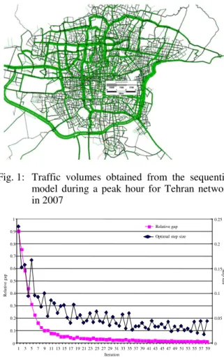
• Assigned (UE assignment) OD matrices of trips with work and educational purposes on Tehran network in TransCAD software. The UE assignment in the Sequential Model (SM) obtained after 76 iterations (ε = 0.01). The outputs of the assignment model were link volumes and travel times. Figure 1 shows traffic volumes that are obtained from the peak hour SM of Tehran network in 2007

Fig. 1: Traffic volumes obtained from the sequential model during a peak hour for Tehran network in 2007

0 0.1 0.2 0.3 0.4 0.5 0.6 0.7 0.8 0.9 1

1 3 5 7 9 11 13 15 17 19 21 23 25 27 29 31 33 35 37 39 41 43 45 47 49 51 53 55 57 59

Iteration

R

el

a

ti

v

e

g

ap

0 0.05 0.1 0.15 0.2 0.25

S

te

p

s

iz

e

Relative gap

Optimal step size

Fig. 2: Relative gap and optimal step size for CTDAM used d = 26 min that was obtained from OD matrices

• The next step involved solving the Tehran network with CTDAM model, using d = 26 min and applicable trip production and attraction of traffic analysis zones

The convergence of the solution to the CTDAM is shown in Fig. 2. As depicted in this figure, after 59 iterations, the Evans algorithm reached relative gap and optimal step size of 0.009924 and 0.044185 respectively. Furthermore, two other convergence criteria were considered, one involving the trip table and another for the link flow array.

For the trip table, a simple criterion is considered in which the Total Misplaced Flow (TMF) is estimated. This is the sum of the absolute differences of zone-to zone OD flows in the main problem and sub problem solutions. If these two measures are equal, then one can conclude that the algorithm has converged with regard to the trip table[19]. TMF estimates for CTDAM model

1 10 100 1000 10000 100000 1000000

1 3 5 7 9 1 1 11 1 2 2 2 2 2 3 3 3 3 3 4 4 4 4 4 5 5 5 5 5 Iteration

T

M

F

0 1000 2000 3000 4000 5000 6000 7000

M

a

x

f

lo

w

c

h

a

n

g

e

Total

Max flow

Fig. 3: Total misplaced OD flow and maximum link flow change for CTDAM

SM flow = 0.6568x + 646.71 R2 = 0.6604 CTDAM flow = 0.8242x + 437.82

R2 = 0.7612

0 1000 2000 3000 4000 5000 6000 7000 8000 9000

0 1000 2000 3000 4000 5000 6000 7000 8000 9000

Observed flow

C

T

D

A

M

a

n

d

S

M

SM CTDAM Linear (SM Linear (CTDAM

Fig. 4: Comparison of CTDAM and SM with observed link flow

are presented in Fig. 3 using the log scale to facilitate the comparison. It is shown that the TMF measure reached a minimum value of 2 persons/hour in the 16th iteration and then remained unchanged.

For the link flow portion of the problem, another convergence criterion that was considered deals with the maximum overall link flow change that is the absolute deviations between the current solution and the solution from the previous iteration[18]. This criterion is also shown in Fig. 3.

Comparative results: Our comparative analysis were based on comparing the predicted daily link flows output from each approach to the observed morning peak hourly link flows where we have 48 links with observed traffic counts in 2006 data from TCTTS[17].

The results of the comparison point out that there is enough correlation between link flows from the CTDAM and observed link flows. The better performance of proposed model (CTDAM) compare to SM grows up of comparison study.

The intercepts of both models are not large, however regression coefficient (slope) from CTDAM is statistically accepted and closer to one compare to SM.

CONCLUSION

The sequential approach used in practice to predict short-run transportation equilibrium has several inherent weaknesses and is internally inconsistent in its models structure. To overcome these deficiencies, this study applied a combined model for the simultaneous prediction of trip distribution and trip assignment to Tehran Metropolitan Area with the goal to perform a comparison between the sequential and simultaneous approaches. The comparison between the solutions of the sequential procedure and combined models remain as a valid research problem that needs to be examined in many urban areas. In this study the CTDAM is used for predicting captive trips on transportation network of Tehran. It was shown that the proposed combined model can notably satisfy several convergence criterions. Furthermore, different evaluation measures are utilized to compare the results of the combined model with a SM.

The modeling results presented in this research suggest that:

• The UE assignment in the CTDAM can be obtained relatively faster than the SM.

• There is enough correlation between link flows from the CTDAM and observed link flows

• When we compare proposed CTDAM and SM with sample observed link flows, CTDAM results (R2, intercept and regression coefficient) are statistically more significant rather than SM

Finally, several avenues for future research have emerged from this study. It appears to be productive to reformulate and apply the model so that it also consists of the modal split step. Furthermore, due to various travel-related constraints (imposed by personal and household characteristics as well as transportation system), the use of the models capable of distinguishing between captive and non-captive trips and considering both trips in a single modeling structure should be explored in future research.

ACKNOWLEDGEMENTS

Authors are thankful to Professor David Boyce for his valuable comments on the first draft of this research. Data and network information used in this study are provided by Tehran Comprehensive Transportation and Traffic Studies Company (TCTTS).

REFERENCES

1. Maruyama, T. and N. Harata, 2005. Incorporating trip chaining behavior in network equilibrium analysis. Trans. Res. Rec., 1921: 11-18.

2. Boyce, D. and H. Bar-Gera, 2004. Multiclass combined models for urban travel forecasting. Net. Spati. Econ., 4 (1): 115-124.

3. Beckmann, M., C.B McGuire and B.C. Winsten, 1956. Studies in the Economics of Transportation. Yale University Press: New Haven, Conn.

4. Suzanne Evans, 1973. Some applications of mathematical optimization theory in transportation planning. Doctoral Dissertation, University of London.

5. Florian, M. and S. Nguyen, 1978. A combined trip distribution, modal split and trip assignment model. Trans. Res. Rec., 12: 241-246.

6. Yosef Sheffi, 1985. Urban transportation networks: Equilibrium analysis with mathematical programming methods. Prentice Hall, Englewood Cliffs, N.J., pp: 164-198.

7. Safwat, K.N.A. and T.L. Magnanti, 1988. A combined trip generation, trip distribution, modal split and traffic assignment model. Trans. Sci., 22 (1): 14-30.

8. Hasan, M.K. and A.H. AlGadhi, 1998. Comparison of simultaneous and sequential transportation network equilibrium models' application to riyadh, Saudi Arabia. Trans. Res. Rec., 1645: 127-132. 9. Maruyama, T., N. Harata and K. Ohta, 2001. The

combined modal split/assignment model in the Tokyo Metropolitan Area. J. Easte. Asia Soc. Trans. Stud., 4 (2): 293-304.

10. Boyce, D. and D. Lohse, 2002. Comparisons of two combined models of urban travel choices: Chicago and Dresden. 42nd Congress of the European Regional Science Association at the University of Dortmund, Dortmund, Germany, ERSA02, pp: 413.

11. Leo Dobes, 1998. Urban transport models: A review. Bureau of Transport Economics, Working Paper 39, Canberra, pp: 7-9.

13. Hugo Pietrantonio, 2001. Land use and transport integrated models- basic relations and solution approaches. Department of Transportation Engineering, Polytechnic School, University of São Paulo, pp: 43-44.

14. Alan G. Wilson, 1970. Entropy in urban and regional modelling, Pion, London.

15. Chu, Y.L., 1999. Network equilibrium model of employment location and travel choices. Trans. Res. Rec., 1667: 127-132.

16. Michael Patriksson, 1994. The traffic assignment problem-models and methods. Linkoping Institute of Technology, Linkoping, Sweden, pp: 104-106.

17. Tehran Comprehensive Traffic and Transportation Plan, 2007. Updating transportation demand and supply data for Tehran. Tehran Comprehensive Transportation and Traffic Studies Co (TCTTS), pp: 56-67.

18. Metaxatos, P., D. Boyce and M. Florian, 1995. Implementing combined model of origin-destination and route choice in EMME/2 system. Trans. Res. Rec., 1493: 57-63.