Equivalent Absorbing Boundary Conditions
for Heterogeneous Acoustic Media
M.L. CASTRO1*, J. DIAZ2 and V. P ´ERON2
Received on November 30, 2013 / Accepted on August 19, 2014
ABSTRACT.In this work, we derive high order Equivalent Absorbing Boundary Conditions EABCs that model the propagation of waves in semi-infinite bilayered acoustic media. Our motivation is to restrict the computational domain in the simulation of seismic waves that are propagated from the earth and transmit-ted to the stratified heterogeneous media composed by ocean and atmosphere. These EABCs are adaptransmit-ted to Hagstrom-Warburton ABCs and appear as first and second order of approximation with respect to a small parameter involved in a multiscale expansion. Computational tests illustrate the accuracy of the first approximate model with respect to the small parameter.
Keywords:artificial boundaries, computational wave propagation, equivalent boundary conditions, hetero-geneous media, acoustic waves.
1 INTRODUCTION
The numerical simulation of geophysical phenomena is of utmost importance in our society. Considering the massive destruction seismic activities can generate, it is crucial to apply science towards a better understanding of the impact of earthquake waves.
Part of the job is to obtain effective models yielding the numerical simulation of seismic activity at an affordable computational cost – observe that running times are a very important factor when dealing with eminent tragedies. On the other hand, a complete description of the physical problem at hand is extremely intricated. In particular, it involves the coupling of elastic and acoustic waves in heterogeneous media, and the absence of viscosity produces waves that travel long distances without changing much their shape or amplitude. This aspect of the problem generates difficulties for the numerical simulation, since the physical domain, if one includes the atmosphere, is unbounded. Moreover, as waves propagate much slower in the atmosphere than in the sea or in the subsurface, one has to consider meshes composed of very thin cells
*Corresponding author: Manuela L. De Castro
1UFRGS – Departamento de Matem´atica Pura e Aplicada, 91509-900 Porto Alegre, RS, Brasil. E-mail: [email protected]
in this region. Since the primary interest is to compute seismograms in the subsurface, it is necessary to consider techniques allowing to reduce at most as possible the computations inside the atmosphere. The imposition of artificial contours and appropriate boundary conditions (BCs) is an aspect to be considered. Among many possibilities, one could use a non-reflecting BC, defined through pseudo-differential operators [1, 2, 3, 4], or choose from a variety of approximate BCs, such as PMLs [5, 6, 7] or Absorbing Boundary Conditions (ABCs) [8, 9, 10, 11, 12, 13]. In this work the Hagstrom-Warburton ABC [10, 14] is chosen. The benefit of implementing non-reflecting BCs is discussed in [8] and it has been proven in [15] that the Hagstrom-Warburton ABC is equivalent to the popular Higdon ABC, with advantages with respect to implementation and computational cost.
However, even when using High-Order BCs, the artificial boundary should be placed at a distance
ǫof the subsurface, in order to avoid spurious reflections. Hence, it is still necessary to mesh the small layer of the atmosphere with very thin cells. In this work, an alternative method is proposed, based on the use of asymptotic techniques in order to obtain Equivalent BCs that we could impose directly at the interface between the atmosphere and the subsurface.
The concept of equivalent boundary conditions (ECs) has become well-known in the mathemat-ical modeling of wave propagation phenomena [16, 17, 18, 19, 20]. Such conditions are usually used to reduce and simplify the computational domain, replacing an exact model that must be applied in the periphery of the domain by an artificial contour and a BC that resembles the effects of the exact model on the part of the domain that was excluded. The main tool for the construc-tion of ECs are two scale asymptotic expansions on the parameter defining the thickness of the layer to be eliminated.
A key hypothesis for the validation of this technique relies on the smallness of the ratio between the thickness of the layer to be eliminated and the remainder of the domain, typically with re-spect to the wavelength. It is worth to notice that the original physical problem inspiring this work does not satisfy such hypothesis. As a matter of fact in the original problem the atmo-sphere layer is an unbounded layer. What motivates this model is that, according to [14], it is possible to approximate the solution in the unbounded domain with any set precision tolerance if one applies an ABC of order high enough. At this stage, therefore, the focus is on the approx-imation of this problem with an absorbing boundary, rather than the physical problem with an unbounded layer.
The originality of this work is the derivation of ECs adapted to Hagstrom-Warburton ABCs, that will be called Equivalent Absorbing Boundary Conditions (EABCs). The EABCs appear as a first and second order approximations (Section 3.2) with respect to the small parameter and which are satisfied by the acoustic pressure. This paper presents a preliminary study that illustrates the feasibility of the approach. It focuses essentially on the formal derivation of EABCs and on the numerical accuracy of low order EABCs.
2 MATHEMATICAL MODELLING
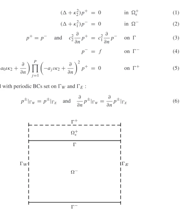
In this work, a region of interest consisting of two media (ocean and atmosphere, for instance) is considered. Starting from a rectangularly shaped, double layered spatial model (see Fig. 1), where the boundariesŴ+,Ŵ−,ŴW andŴEare artificial. The focus here is on the treatment ofŴ+
defined as an absorbing boundary, whereas the countoursŴW andŴE are modeled as periodical
boundaries and a Dirichlet boundary condition (BC) is set onŴ−(4). The Dirichlet data f set onŴ−can be thought as a forcing term generated by waves that were transmitted to−from an elastic media underneathŴ−. The goal is to obtain a reduced model for the acoustic pressure
p−in−of a wave with frequencyωthat propagates with velocityc1in−and is transmitted to+ǫ (ǫis the thickness of the layer+ǫ) with velocityc2. Denoting by κ1 = cω1, κ2 = cω2 one has
(+κ22)p+ = 0 in +ǫ (1)
(+κ12)p− = 0 in − (2)
p+= p− and c22 ∂
∂np
+ = c2 1
∂ ∂np
−
on Ŵ (3)
p− = f on Ŵ− (4)
−a0ıκ2+ ∂ ∂n
P
j=1
−ajıκ2+ ∂ ∂n
2
p+ = 0 on Ŵ+ (5)
complemented with periodic BCs set onŴW andŴE :
p±|ŴW =p
±|
ŴE and
∂
∂np
±| ŴW =
∂
∂np
±|
ŴE (6)
The time-harmonic wave field is characterized by using the Helmholtz equations (1)-(2) for the acoustic pressures p+ in+ǫ and p− in−. The transmission conditions (3) require that the pressures and the normal velocities match on the interfaceŴ; the first condition results from the equilibrium of forces onŴ. The boundary condition (5) is a Higdon BC [9] and coefficientsaj ∈ (0,1] are given parameters. Rewriting (5) according to the Hagstrom-Warburton formulation [10, 14, 15], adapted to the problem stated in the frequency domain, BC (5) becomes
−a0ıκ2+ ∂ ∂n
p+ = −ıκ2φ1 (7)
−ajıκ2+ ∂ ∂n
φj =
−ajıκ2− ∂ ∂n
φj+1, j =1, . . . ,P (8)
φP+1 = 0. (9)
Here the functionsφj (j=1, . . . ,P+1) are auxiliary variables, defined onŴ+and in a vicinity
V which is located above the domain+
ǫ, and we assume that (7)-(8)-(9) hold onŴ+∪V.
Then, following the procedure stated in [10], we have that(+κ22)φj =0 inV; what leads to
the elimination of the normal derivatives with respect to the boundaryŴ+. This yields rewriting (7)-(9) as
−a0ıκ2+ ∂ ∂n
p+ = −ıκ2φ1 on Ŵ+ (10)
−κ22L = M ∂ 2
∂x2+2 ∂2 ∂x2p
+e
1 on Ŵ+ (11)
where=(φ1, . . . , φP)T andL,Mare tridiagonal matrices P×P whose entriesli j andmi j
depend on the parametersaj. More specifically,
l11=1+a12+2a1a0, l12=1−a12, lj,j+1=aj−1(1−a2j), j =2, ...,P−1
lj,j−1=aj(1−a2j−1), lj j =aj(1+a2j−1)+aj−1(1+a2j), j=2, ...,P
m11=a1+a0, m12 =a0, mj,j+1=aj−1, j =2, ...,P−1
mj,j−1=aj, mj j =aj+aj−1, j =2, ...,P
Unlike (7)-(8)-(9), the formulation (10)-(11) involves only the values of φj on the boundary
Ŵ+. This decreases considerably the computational cost of numerical simulations. Finally the problem of interest writes (1)-(4) with the BCs (6) and (10)-(11).
3 MAIN RESULTS – EQUIVALENT CONDITIONS
3.1 Formal derivation of equivalent conditions
First step: a multiscale expansion. The first step consists to derive a multiscale expansion for the solutionp+ = p+ǫ, p− = pǫ−and=ǫ of the problem (1)-(4) complemented with the
BCs (6)-(10)-(11): it possesses an asymptotic expansion in power series of the small parameterǫ
p+(x) = p+0(x;ǫ)+ǫp1+(x;ǫ)+O(ǫ2) in +ǫ, p+j (x;ǫ)=ᒍj
x,y ǫ
;
p−(x) = p−0(x)+ǫp1−(x)+O(ǫ2) in −;
(x, ǫ) = 0(x)+ǫ1(x)+O(ǫ2). (12)
Herex=(x,y)∈R2are the cartesian coordinates. The “profiles”ᒍj are defined onŴ×(0,1)
whereas the termsp−j (resp.j) are defined in−(resp. onŴ).
Second step: construction of equivalent conditions. The second step consists to identify a simpler problem satisfied by the truncated expansions
p−k,ǫ:= p−0 +ǫp1−+ǫ2p−2 + · · · +ǫkp−k in −
k,ǫ=0+ǫ1+ǫ22+ · · · +ǫkk on Ŵ
up to a residual term inO(ǫk+1). The simpler problems are stated in Section 3.2 whenk∈ {0,1}. There holds (at least) formal estimates
p−ǫ −pkǫ− =O(ǫk
+1)
(13)
wherepǫksolves the simpler problem, anequivalent model of order k.
3.2 Main results – Equivalent models
In the framework above, the equivalent models (EABCs) of orderk∈ {0,1}are stated.
Order 0 model. p0−and0(x)=(φ01, . . . , φ0P)T(x)solves the problem
p−0 +κ12p0− = 0 in −
−a0ıκ2+ c1 c2 2 ∂ ∂n
p0− = −ıκ2φ01 on Ŵ
−κ22L0−M∂ 2
∂x20 = 2
∂2 ∂x2p
−
0e1 on Ŵ
p0− = f on Ŵ−,
(14)
complemented with periodic BCs onŴW andŴE.
Order 1 model. pǫ1and1ǫ(x)=(φǫ1, . . . , φǫP)T(x)solves the problem
pǫ1+κ12p1ǫ = 0 in −
−a0ıκ2+ c1 c2 2 ∂ ∂n
p1ǫ = (−ıκ2+ǫa0κ22)φǫ1+ǫ
∂2
∂x2p1ǫ+κ22(1−a 2 0)p
1
ǫ
on Ŵ
−κ22L1ǫ−M∂2
∂x2 1
ǫ = 2
(1+ǫa0ıκ2)∂ 2
∂x2p 1
ǫ −ǫıκ2 ∂ 2
∂x2φ 1
ǫ
e1 on Ŵ
p1ǫ = f on Ŵ−
3.3 Derivation of equivalent models
After applying a change of scale y→Y = yǫ in+ǫ, equations (1)-(4) complemented with the BCs (10)-(11) become
ǫ−2 ∂2
∂Y2 +
∂2
∂x2 +κ 2 2
ᒍ+(x,Y) = 0 in Ŵ×(0,1)
(+κ12)p− = 0 in −
ᒍ+ = p− on Ŵ (Y =0)
c22ǫ−1∂∂Yᒍ+ = c21∂∂np− on Ŵ (Y =0)
p− = f on Ŵ−
−a0ıκ2+ǫ−1∂∂Yᒍ+(x,1) = −ıκ2φ1(x)
−κ22L(x, ǫ) = M∂2
∂x2(x, ǫ)+2
∂2 ∂x2ᒍ
+(x,1)e
1
Hereᒍ+(x,yǫ)=p+(x,y)and=:(φ1, . . . , φP)T.
Equations for the first asymptotics.Substituting the ansatz (12) forp+,p−andinto previous equations and performing the identification of terms with the same power ofǫ, a collection of equations for the coefficients(p−j,ᒍj)andj is obtained. One finds that(p0−,ᒍ0)and0 = (φ01, . . . , φ0P)T solve
∂2 ∂Y2ᒍ
+
0 = 0 in Ŵ×(0,1) (15)
(+κ12)p0− = 0 in− (16)
ᒍ+0 = p0− onŴ (Y =0) (17)
c22 ∂
∂Yᒍ
+
0 = 0 on Ŵ (Y =0) (18)
p−0 = f on Ŵ− (19)
∂ ∂Yᒍ
+
0(x,1) = 0 (20)
−κ22L0(x) = M ∂2
∂x20(x)+2 ∂2 ∂x2ᒍ
+
0(x,1)e1 (21)
with periodic BCs set onŴW andŴE, and(p1−,ᒍ1, 1)solves
∂2 ∂Y2ᒍ
+
1 = 0 in Ŵ×(0,1) (22)
(+κ12)p1− = 0 in − (23)
ᒍ+1 = p1− on Ŵ (Y =0) (24)
c22 ∂
∂Yᒍ
+
1 =c 2 1
∂ ∂np
−
p−1 = 0 on Ŵ− (26)
−a0ıκ2ᒍ+0(x,1)+ ∂ ∂Yᒍ
+
1(x,1) = −ıκ2φ 1
0(x) (27)
−κ22L1(x) = M ∂2
∂x21(x)+2 ∂2 ∂x2ᒍ
+
1(x,1)e1 (28)
with periodic BCs set onŴW andŴE.
Construction of the first asymptotics and equivalent conditions. From (15), (18) and (20),
ᒍ+0 must have the form
ᒍ+0(x,Y)=α0(x).
Equation (17) providesα0(x)=p−0(x,0). Also, from (22) one has
ᒍ+1(x,Y)=β0(x)+β1(x)Y.
Additionally, (25) provides
c22β1(x)=c21 ∂ ∂np
−
0(x,0) whereas equation (27) rewrites as
−a0ıκ2α0(x)+β1(x)= −ıκ2φ01(x).
Therefore one gets
c22a0ıκ2p0−(x,0)=c21 ∂ ∂np
−
0(x,0)+c 2
2ıκ2φ01(x).
Finally (21) andᒍ+0(x,Y)=α0(x)=p−0(x,0)yield
−κ22L0(x)=M ∂2
∂x20(x)+2 ∂2 ∂x2p
−
0(x,0)e1,
where
0(x)=(φ01, . . . , φ0P)T(x)
providing the order 0 model (14). Further computations also provide the order 1 model, Sec-tion 3.2.
4 NUMERICAL RESULTS
For the model problem considered, our findings indicate that the use of an equivalent absorbing boundary condition can be a viable and effective alternative for numerical simulation; mainly for the gain in computational cost provided by such conditions.
The numerical solution was obtained using the Interior Penalty Discontinuous Galerkin Method [21] withP3elements. The normal derivative of p
Finally, the third equation of (14) is discretized by applying a 1D IPDG method onŴ. Hence, for
P=1, we have to solve a linear system that reads as
(K2D+κ12M2D)P+B2D1D =F
B1D2DP+(K1D+κ22M1D)=0,
(29)
wherePandare the vectors containing respectively the value of p0andφ01at their degrees of freedom (recalling thatφ01is a 1D function defined only onŴ). M2DandK2D are the mass and
stiffness matrices obtained by the 2D IPDG method, M1D andK1D are the mass and stiffness
matrices obtained by the 1D IPDG method and B2D1D and B1D2D are the two matrices that
ensures the coupling between the two equations.
In a test problem, we have compared the solution of (1)-(4) with the boundary conditions (10)-(11)-(6) for p−in−with the solutionp0obtained using the order 0 model (14) here presented. The Dirichlet data
f =exp
iω c1
(xcosθ )
,
models the diffraction of an incident wave of frequencyω=10 Hz and hitting the boundaryŴ−
at an angle ofθ = 5π
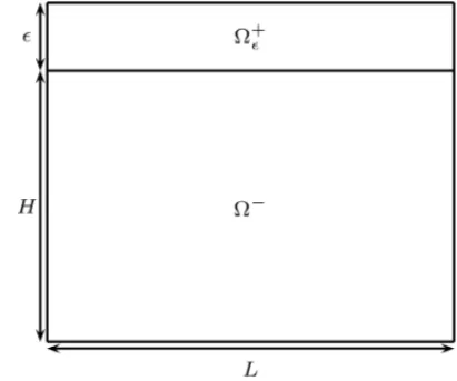
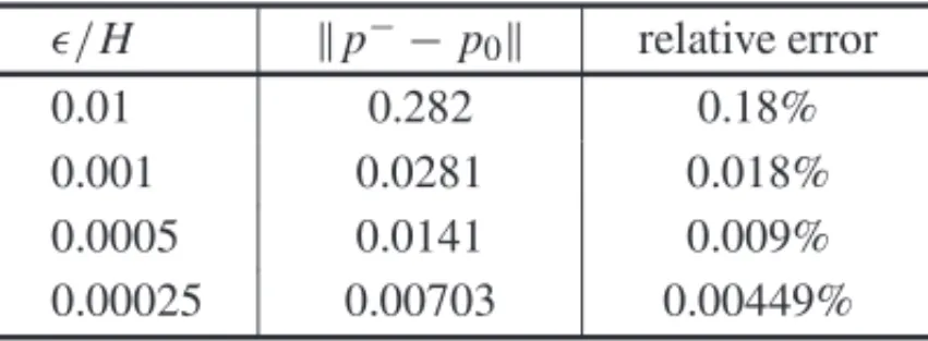
12. Takingc1/c2 =2, P =1 (witha0 =1 anda1 =1) and modelling f as an incident wave, we have reached relative errors below 0.2%, considering the ratio of 10−2 forǫ/H, whereH is the thickness of the layer−(see Fig. 2). The results are summarized for various values ofǫ/Hin Table 1. The convergence rate coincides with the formal estimate (13) whenk=0. It is worth to notice that in order to satisfy periodicity, the parameters chosen must relate to the widthLof the domain respectingL = 2qπc1
ωcosθ, whereq ∈ IN. Besides, there should
be some extra care in the choice ofω: it should not be too big (else the conditionǫ ≪ 2πc1,2
ω
will not be satisfied) or too small (this would demand a very large domain, since Lis inversely proportional toω). In the test case presented, c1 = 1500 m/s andL was set to approximately 1885 m. The triangular double layer meshes (necessary to compute p0) used had around 105 elements, with triangle sizes set around 0.08 in the thin layer and its vicinity.
Table 1: Comparative test between p−and p0. p−−p0 refers to the euclidean distance between p−andp0in a sam-ple of 1000 points over a regular mesh on the domain−.
ǫ/H p−−p0 relative error
0.01 0.282 0.18%
0.001 0.0281 0.018%
0.0005 0.0141 0.009%
0.00025 0.00703 0.00449%
5 CONCLUSION
We have derived high order Equivalent Absorbing Boundary Conditions EABCs that model the propagation of waves in semi-infinite bilayered acoustic media. The numerical results illustrate the fact that forP =1 andk =0, the EABC models very accurately problem (1)-(4) with the conditions (10)-(11) and (6), as soon asǫ/H ≤ 0.0005. Obviously, for such small values of
ǫ/H, this problem is not able to reproduce accuratly the case where the upper media is infinite. Hence, the next step will be to study the effect ofPon the solution. This will provide a minimal valueP0for which the EABC in (14) is efficient enough. Finally, the order 1 model is expected to allow for considering higher values ofǫ/Hand to provide a smaller value forP0, which would reduce the number of auxiliary functionsφand the computational costs.
RESUMO. Partindo de uma modelagem no dom´ınio de frequˆencias, utilizamos condic¸˜oes de contorno artificiais de Higdon e aproximac¸˜oes assint´oticas para obter condic¸˜oes de
con-torno equivalentes que viabilizem a reduc¸˜ao do dom´ınio computacional para a simulac¸˜ao da propagac¸˜ao de ondas em meios ac ´usticos heterogˆeneos. A motivac¸˜ao para este trabalho ´e a
obtenc¸˜ao de condic¸˜oes de contorno artificiais e aproximadas para a simulac¸˜ao da propagac¸˜ao de ondas s´ısmicas, oriundas do interior da terra e transmitidas ao meio ac ´ustico heterogˆeneo
composto pelos oceanos e pela atmosfera.
Palavras-chave:contornos artificiais, condic¸˜oes de contorno equivalentes, ondas ac ´usticas, meio heterogˆeneo.
REFERENCES
[1] B. Alpert, L. Greengard & T. Hagstrom. “Rapid evaluation of nonreflecting boundary kernels for time-domain wave propagation”.SIAM Journal on Numerical Analysis,37(4) (2000), 1138–1164. [2] T. Hagstrom & S. Hariharan. “A formulation of asymptotic and exact boundary conditions using local
operators”.Appl. Numer. Math.,27(1998), 403–416.
[4] M.J. Grote & J.B. Keller. “Exact nonreflecting boundary conditions for the time dependent wave equation”.SIAM Journal on Applied Mathematics,55(2) (1995), 280–297.
[5] J.P. B´erenger. “A perfectly matched layer for the absorption of electromagnetic waves”.J. Comput. Phys.,114(1994), 185–200.
[6] S. Abarbanel & D. Gottlieb. “A mathematical analysis of the pml method”.Journal of Computational Physics,134(2) (1997), 357–363.
[7] I. Navon, B. Neta & M. Hussaini. “A perfectly matched layer approach to the linearized shallow water equations models.”Monthly Weather Review,132(6) (2004).
[8] D. Givoli & B. Neta. “High-order nonreflecting boundary scheme for timedependent waves”.J. Com-put. Phys.,186, 24–46, March 2003.
[9] R.L. Higdon. “Absorbing boundary conditions for difference approximations to the multidimensional wave equation”.Mathematics of computation,47(176) (1986), 437–459.
[10] T. Hagstrom & T. Warburton. “A new auxiliary variable formulation of high-order local radiation boundary conditions: corner compatibility conditions and extensions to first-order systems”.Wave motion,39, 327–338, April 2004.
[11] D. Givoli. “High-order local non-reflecting boundary conditions: a review”.Wave Motion, 39(4) (2004), 319–326.
[12] V. van Joolen, B. Neta & D. Givoli. “A stratified dispersive wave model with high-order nonreflecting boundary conditions”.Comput. Math. Appl.,48(7-8) (2004), 1167–1180.
[13] J.M. Lindquist, F.X. Giraldo & B. Neta. “Klein-Gordon equation with advection on unbounded do-mains using spectral elements and high-order non-reflecting boundary conditions”.Appl. Math. Com-put.,217(6) (2010), 2710–2723.
[14] T. Hagstrom, M.L. De Castro, D. Givoli & D. Tzemach. “Local highorder absorbing boundary condi-tions for time-dependent waves in guides”.Journal of Computational Acoustics,15(1) (2007), 1–22. [15] D. Givoli, T. Hagstrom & I. Patlashenko. “Finite element formulation with high-order absorbing boundary conditions for time-dependent waves”.Computer Methods in Applied Mechanics and En-gineering,195(29) (2006), 3666–3690.
[16] B. Engquist & J.-C. N´ed´elec. “Effective boundary conditions for acoustic and electromagnetic scat-tering in thin layers”. Technical Report of CMAP 278, Centre de Math´ematiques Appliqu´ees, (1993).
[17] A. Bendali & K. Lemrabet. “The effect of a thin coating on the scattering of a time-harmonic wave for the helmholtz equation”.SIAM Journal on Applied Mathematics,56(6) (1996), 1664–1693. [18] T. Abboud & H. Ammari. “Diffraction at a curved grating: TM and TE cases, homogenization”.J.
Math. Anal. Appl.,202(3) (1996), 995–1026.
[19] O.D. Lafitte. “Diffraction in the high frequency regime by a thin layer of dielectric material i: The equivalent impedance boundary condition”.SIAM Journal on Applied Mathematics,59(3) (1998), 1028–1052.
[20] V. P´eron. “Equivalent boundary conditions for an elasto-acoustic problem set in a domain with a thin layer”.ESAIM: Mathematical Modelling and Numerical Analysis, EDP Sciences,48(5) (2014), 1431–1449.
[21] M.J. Grote, A. Schneebeli & D. Sch¨otzau. “Interior penalty discontinuous Galerkin method for