I
I
DE
D
EO
OL
LO
OG
GI
IC
CA
A
L
L
C
CH
HA
AN
N
GE
G
ES
S
A
AN
ND
D
T
TA
AX
X
S
ST
TR
RU
UC
C
TU
T
UR
R
E
E
:
:
L
LA
AT
TI
IN
N
AM
A
M
ER
E
R
IC
I
C
A
A
N
N
C
CO
OU
UN
NT
TR
RI
IE
ES
S
D
DU
UR
RI
IN
NG
G
T
TH
HE
E
N
N
IN
I
N
E
E
TI
T
IE
ES
S
C
LAUDIOR
IBEIRO DEL
UCINDAP
AULOR
OBERTOA
RVATEDezembro
de 2007
T
T
e
e
x
x
t
t
o
o
s
s
p
p
a
a
r
r
a
a
D
TEXTO PARA DISCUSSÃO 168 • DEZEMBRO DE 2007 • 1
Os artigos dos Textos para Discussão da Escola de Economia de São Paulo da Fundação Getulio Vargas são de inteira responsabilidade dos autores e não refletem necessariamente a opinião da
FGV-EESP. É permitida a reprodução total ou parcial dos artigos, desde que creditada a fonte.
I
Id
de
eo
ol
l
o
o
g
g
i
i
ca
c
al
l
c
ch
ha
an
ng
ge
es
s
a
a
n
n
d
d
t
ta
a
x
x
s
st
tr
ru
uc
ct
tu
ur
re
e:
:
L
La
at
ti
in
n
A
Am
me
e
r
r
i
i
ca
c
an
n
c
co
o
u
u
n
n
tr
t
ri
ie
es
s
d
du
ur
ri
in
ng
g
t
th
h
e
e
n
ni
in
ne
et
ti
i
e
e
s
s
∗Cláudio Ribeiro Lucinda Getúlio Vargas Foundation 1
Paulo Roberto Arvate
Getúlio Vargas Foundation and Pontifical Catholic University 2
Abstract
Sabatini (2002) and Roberts and Wibbles (1999) pointed out that voters in Latin American countries are no longer choosing according to their ideological preferences. Ashworth and Heyndels (2002) showed that the tax choice in OECD countries does not follow the ideological pattern of party preferences. The most robust result of this work shows that the tax choice in Latin American countries still depends on this ideological preference. We also verified that changes in the tax structure depend on changes both in the tax burden and the openness of the economy.
1. Introduction
Recent literature has drawn attention to the fact that the classification of Latin American
political parties as left-wing or right-wing is becoming less meaningful.3 Roberts and Wibbels
(1999) pointed out that this change was the result of the growth of an unorganized working class
that is part of the informal sector of the economy. According to them, this not only affects the
parties, but also the stability of the political system. 45
This result is at odds with another line of research that seeks to assess the effects party
ideologies have on tax structure. Pommerehne and Schneider (1983) state that, when elected,
governments with a different ideological orientation from their predecessors change taxation in a
way that is consistent with their own preferences. 6
Considering the strong tradition that characterizes the parties in ideological terms in
Latin American countries 7 and the establishment of a full democratic system at all government
levels in the biggest and most populous countries of the continent, could it be that this loss of the
ideological characteristics of the political actors also has an effect on the tax choice? In the
current situation are there no longer baskets of taxes that differentiate the left-wing from
right-wing parties? If the parties reflect the choice of the electorate, and if they are not choosing
parties due to ideology, is the tax structure accompanying this trend?
These questions provide the goal for this work: to investigate whether the ideological
changes in governments imposed changes on tax structure according to these ideologies. If this
occurred in Latin American countries, should we look with caution at the assertion that voters no
longer express their choice according to traditional ideological views?
This is not a question that can be easily answered, because it would imply clear
definitions on what basket of taxes are supposed to belong to left-wing or right-wing
debatable. However, even if we do not impose such assumptions, it is still possible to check
whether changes in the tax structure after elections can be traced to ideological changes. We
merely have to assume that up until the election, the existing basket of taxes reflects the choice
of the government in power. Whenever there is an ideological change after the election, we have
to check if this was accompanied by a change in the tax structure. We still will not be able to
establish which basket of taxes belongs to each ideological type of government, but there will be
evidence on the relationship between ideological and tax structure changes.
In addition to this introduction four sections will be necessary for this goal. In the second
section we shall show the movement in the tax structure in Latin American countries. The first
step in the analysis is to determine a measure for classifying the changes in tax structure. We
chose the methodology used by Ashworth and Heyndels (2002) that is able to capture changes
in the tax structure. In the third section we shall discuss the economic and political causes found
in literature that justify this movement. Empirical evidence in the fourth section will lend support
to our discussion on these issues, so that in the last section we can highlight our main
conclusions.
2. Was there any change in tax structure in Latin American countries in the
nineties?
Ashworth and Heyndels (2002) constructed an index that was able to reflect changes
occurring in tax structure and they tested it using a sample of 19 OECD countries between 1965
and 1995.8 The equation that represents the index – the tax turbulence index (TURB) – can be
seen below:
∑
= −
− =
∆
= n
j
i t j i
t j i
t i
t R R R
TURB
1
1 , ,
where
• each i t j
R , of the vector ( 1, , 2, ,... , )
i t n i
t i
t i
t R R R
R =
denotes the share of each of the j taxes in year t as a proportion of the total amount collected by country i;
• 1≥ 1i, ≥0
t
R ;
• The sum of these shares cannot be greater than the whole:
∑
, =1i t j
R
.
If the results of this index are close to zero the tax structure in year t will have been
equal to the tax structure in t –1 and if they reach two the tax structure will have been completely
altered.
Ashworth and Heyndels (2002) used the annual data on the structure of national taxes,
as published by the OECD. The classification of taxes is very detailed and based on 60 different
sources. They chose to work with two groups of taxes, which is the reason why their results were
presented in two indices. TURBULENCE 6 reflected the variation of the six main groups of taxes
(code ‘000’) and TURBULENCE 19 reflected the change in nineteen tax sub-groups (code ‘00’).9
Their results showed the existence of a change in tax structure over time for both the group of
countries as a whole, as well as for each one of them individually.
We tried to reproduce just one of them (similar to what they had considered with the
code ‘000´)10 for Latin American countries. We used data from the consolidated central
government, and the data source was the Government Finance Statistical Yearbook (GFSY). 11
The charts 1 and 2 show the turbulence index in two different ways, which gives us an
idea of how tax composition behaved in fourteen Latin American countries in the nineties
(1991-1999).12
Insert the chart 1 here
We can see in Chart 1 that there was movement in tax structure, although there is not
clear trend in the average turbulence index. Although the work of Ashworth and Heyndels (2002)
America is greater than for OECD countries. In Chart 2 we can see the average turbulence
index, for each country during the same period.
Insert the chart 2 here
Only Brazil and Chile presented a degree of turbulence compatible with that of OECD
countries, and for the other ones the index was considerably higher. Given the fact that there
was a change in the tax structure in Latin American countries greater than the one found for
OECD countries, the causes for this movement must be questioned.
3. Causes of tax changes: a theoretical viewpoint.
In traditional neo-classical literature it is assumed that an optimal fiscal policy implies a
smoothing of tax rates over time. In the version à la Mankiw (1987) this results in equalization of
the social marginal cost of all taxes over time.13 If this result were to prevail it would be very
difficult to verify a change in tax structure over time. On the other hand, the literature also
discusses whether this result has any empirical validity considering that: 1) it is impossible to
maintain the share of each tax, given the changes in the various tax bases;14 2) even if the first
problem is circumvented, when we include the problem of the uncertainty in the evolution of
expenditure, there can be no assurance that changes in total revenue are not accompanied by
changes in the structure of taxes in order to satisfy the inter-temporal budget constraint15 and
finally; 3) if the total revenue changes, we cannot fail to consider the political cost of the choice of
taxes. In their choice politicians are supposed to consider the relative influence of the electorate
on whom the taxes will be levied, and not only the deadweight losses from taxation.16 This choice
can certainly change the initial structure of tax collection.
These criticisms opened up the possibility of investigating which economic and political
rate of GDP growth, inflation, the level and the change of openness in the economy will be
considered to be among the economic causes for this.
We summarize the possible determinants of Latin American tax structure countries on
the table below.17 The sign and timing of the expected effect will be presented. Election years will
be presented on the E column, non-election years will be presented on the t E - n to t E + n.
Insert the table 1 here
Alterations in the total tax burden imply changes in the tax structure, as a result of the
criticisms already presented: 1) alterations in the total tax burden, in order to adapt to the level of
public spending, do not automatically guarantee maintenance of the shares of the various taxes
on the total, and 2) alterations in the total tax burden would lead politicians to a new choice on
which groups the taxes should be levied.
In the results of Ashworth and Heyndels (2002) we can see that changes in the total tax
burden caused changes in the tax structure on OECD countries. We expect that changes in the
total tax burden determine positive changes on tax structure.18
It is also argued in literature that alterations in the rate of GDP growth (in absolute
terms)19 could provoke changes in tax structure. This occurs because the basis for the collection
of each tax may react in a different way to this change (elasticity).20 If the same tax rate is
maintained, with differences in the response of the tax base caused by alterations in the rate of
GDP growth, there will be certainly changes in the collection of each tax and therefore in the tax
structure. Therefore, we would expect the tax base to change due to alterations in the growth
rate of GDP. In the study of Ashworth and Heyndels (2002) the coefficient of this variable was
not significant at the 10% level in the TURBULENCE 6 index. A significant and positive
coefficient was only found in the TURBULENCE 19 index. Wibbels and Arce (2003) do not find a
result, we will expect that changes in the GDP growth to determine changes (positive) on tax
structure.
Inflation would have a similar effect to those described for the rate of GDP growth. An
alteration in the rate of inflation (in absolute terms) would also cause different responses to the
tax base of each of the taxes. We can observe that inflation led to a variation in the total tax
burden (at all levels of government) in one of the significant results from Perotti and Kontopoulos
(1999) between 1960 and 1973.22 Ashworth and Heyndels (2002) find a significant positive effect
of inflation on the tax structure. On the other hand, Steinmo (1993) pointed out that the tax code
on the OECD countries was indexed to reduce inflationary losses. Latin American countries have
had a hard history concerning inflation. The high or hyperinflation these countries lived through
implied differences in response of each tax basis, therefore changing the tax structure and
increasing turbulence.
The fundamental difference between countries with low inflation and high (hyper)
inflation when it comes to tax collection in real terms lies in the time that elapses until the
effective collection of the taxes. Differences in the rate of inflation will determine different levels
of tax in real terms. Two responses are possible: 1) If there is indexation on the tax structure, this
mechanism would be able to neutralize part of the inflationary effects on the real tax collection
(Tanzi effect) – a hypothesis as found in Steinmo (1993);23 2) If the main concern of the
government is on inflationary tax, the tax collection would be reduced in the real terms (the same
Tanzi effect). 24 We do not know which effect prevailed on tax structure of Latin American
countries given this history.
Another factor that would have an influence on tax structure would be the level of
openness of the economy.25 A greater openness in the economy would reduce the changes in
government when it comes to tax choices. The tax structure has to accompany the tax structure
of the countries with which the country has commercial relationships in order to avoid a loss of
competitiveness. However this is not the only way in which the degree of openness may affect
the tax structure. As Ashworth and Heyndels (2002) said:
“ openness may create turbulence by forcing countries to adapt their structure as a
reaction to fiscal externalities from its trade-partners´ policies. As such (absolute) changes in
openness will be positively related to turbulence.” (page 355).
Consequently a change in the degree of openness would also influence the composition
of tax. In the case of OECD countries, both the level, as well as a change in openness, did not
present a significant coefficient to explain the behavior of the tax structure on OECD countries. It
is necessary to remember that a large number of the Latin American countries in this sample
were relatively closed to trade until the mid-eighties. The opening of the economy in the nineties
maybe had a positive influence on the tax structure because these economies would have to
adapt their taxes to the standards of their commercial partners. 26 In this case, the level of
openness would determine a decrease on tax structure changes. On the other hand, changes on
the degree of openness would provoke a significant increase on tax structure changes of Latin
American countries.
Given that the tax structure does not only respond to economic causes but to political
factors, elections, changes in the ideology of government and dispersion of political power are
also factors that must be taken into consideration.
As regards elections, there are two possible effects: 1) an increase in tax change due to
opportunistic manipulation; the incumbent policymaker tries for re-election and 2) a reduction in
The model constructed by Rogoff (1990) to show differences in signaling to the voters
through spending is a useful theoretical structure for understanding opportunistic manipulation.27
Applying these results to the case of taxes, Ashworth and Heyndels (2002) showed that the
policymaker might change the structure of taxes during election years in order to temporarily
signal his competence: income and consumption taxes would be reduced and corporate tax
would be increased. The voters, who have more resources to spend at that moment, would only
perceive the perverse effect of the tax increase on companies after the election. This would
induce them to vote for the incumbent policymaker.
This same signaling structure can be used to understand economic populism in Latin
American countries during the seventies and eighties as a new opportunistic manipulation
strategy.28 In trying to understand the hyperinflationary processes in Latin America in this period,
Dornbusch and Edwards (1989) coined the term for the economic version of populism, the
so-called “economic populism”. According to these authors, with immediate growth and income
distribution objectives, at a time of excessive idle capacity and no problems in external accounts,
the policymakers promoted an expansionist fiscal policy without worrying about its inflationary
financing effects.29 30 When this initial expansionary phase was over, the hyperinflationary
process led to successive crises, which ended in orthodox policies with the gains achieved
rapidly disappearing.3132 Clearly this was a temporary sign of competence whose effects in the
long run were not perceived by the citizens.
Despite not including the electoral moment in their description of the populist cycle, 33
this type of populism can clearly be understood as manipulation - a signal of temporary
competence. Just as Roberts (1995) and Knight (1998) developed the idea that populism
transformed itself, economic populism could have been transformed and found a new form of
described by Ashworth and Heyndels (2002), by means of taxes.If economic populism, in this
modified version, used this strategy the elections would cause changes in tax structure. 35
On the other hand, considering the fixed costs that a change in the tax structure might
bring in terms of election success, there might be no movement in the tax structure. Changes
might create uncertainty and attract the special attention of the media about who the real
taxpayers are (Peters,1991), or who the real losers would be. Certainly this could be considered
as one of the costs of change for the politicians, particularly if the losers are numerous
(Messere,1993). If this is the case, election years might mean inertia as far as tax changes are
concerned (Rose,1985). Thus, the effect of an election year on the tax structure would be nil.
Ashworth and Heyndels (2002) observed that the election had a negative impact on tax
structure of OECD countries. This result corroborates the idea that in election year’s changes do
not occur in the tax structure because of the cost perceived by the politicians in the period prior
to the election. 36 Thus, two opposing results can be expected on Latin American countries:
either a decrease or an increase on tax structure changes on the electoral year.
With the change in ideological regime we might expect to capture the effects of party
preferences. If politicians represent party and ideological preferences and they prefer a certain
tax structure, they might change it when they are in power after the elections (Pommerehne and
Schneider, 1983). The literature point out this variable was not significant on the tax structure of
OECD countries. On the other hand if the idea of Sabatini (2002) is correct, because of the
reasons presented by Roberts and Wibbels (1999), ideological change should not be reflected in
any change in tax structures in Latin American countries after elections. 37
Finally fragmentation of political power would capture the dispersion of power. According
to Roubini and Sachs (1989) political fragmentation makes budget adjustments difficult at times
fragmentation leads to indecision we might expect that a greater dispersion of political power
would lead to less movement in tax structure. Admitting to the criticisms of Edin and Ohlsson
(1991) about the scale of power dispersion put forward by Roubini and Sachs (1989),38 Ashworth
and Heyndels (2002) constructed three dummies39 to check the independent effect of three
forms of dispersion of power on tax structure.40 None of these dummies was significant to explain
the behavior of tax structure 41 We will expect Latin American countries a decrease of changes
on tax structure following an increase of fragmentation of political power.
4. Empirical analysis
In this section we shall test the effect of economic and political variables on the
turbulence index as calculated in the second section. We shall work with a sample of eleven
countries between the years 1991 and 1999. 42 Our basic specification will be:
i t i t i t i t i t i t i t i t i t t i t i t t i t t i t t i i t RE RS ELEI RS RS RE ELEI OP OP IPC GDP TB TURB ε β β β β β β β β β β β + + + + + + + + + + + + = − − − − − − − − ) * ( ) *
( 1 10 1
9 1 8 1 7 6 1 , 5 4 1 , 3 1 , 2 1 , 1 0 (2)
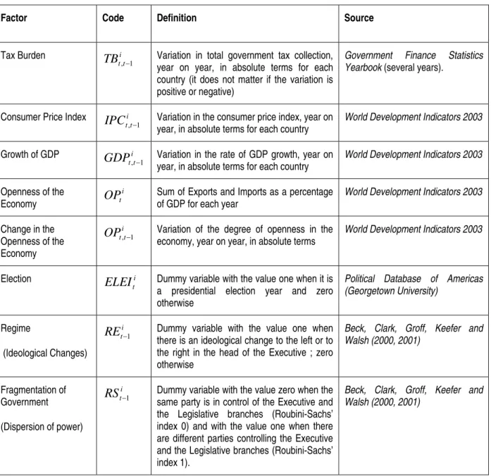
Subscript i represent the country and subscript t represents the year. The definition and
sources of each of the variables are set out in the following table:
Insert Table 2 here
In Appendix 1, table A.1.1, we present the descriptive statistics of each of these
variables.
We will not construct the electoral dummy ( i t
ELEI ) in the same way as proposed in Alesina et
alli (1992, 1993) – that characterizes the different impacts arising from an election occurring in
the first or second half of the year – because the database that was used for constructing the
lack of information we were unable to reproduce the construction of Ashworth and Heyndels
(2002) in relation to regime change ( i t
RE−1): 43
“It equals 1 in year t-1 or in the second half of t-2. The idea is that new government which comes
into power in the first half of the year can adapt the tax code in the second half of that year,
changing tax revenues the year after.” (page 358)
As there is also no classification of the fragmentation of political power ( i t
RS−1) for Latin
American countries in the work of Roubini and Sachs (1989), we chose to construct a single
variable to represent it:44 a dummy with the value zero when the same party controls the
Executive and Legislative branches (this would be Roubini-Sachs’ index 0) and the value one,
when there are different parties controlling the Executive and Legislative branches (this would be
Roubini-Sachs’ index 1). 45 The value zero will be interpreted as cohesion and the value one as
dispersion of power. Ashworth and Heyndels (2002) also included in their tests the interaction
between the fragmentation of power, both with the electoral year ( i t i
t ELEI
RS −1* ) as well as
with the change in regime ( i t i t RS
RE−1* ). This procedure was the same used in Roubini and
Sachs (1989) and its objective is to check whether, when these last two situations are present,
the variable representing dispersion of power would weaken or strengthen its effect on the tax
structure. We used the lagged value of the fragmentation variable on the ( i t i
t ELEI
RS −1* )
interaction. In Ashworth and Heyndels (2002) the interaction ( i t i
t ELEI
RS −1* ) had a positive and
significant sign both using the TURBULENCE 19 index as well as the TURBULENCE 6 index
(even after changing the definition of the fragmentation of power dummy variable). This was an
opposite sign to the one obtained in the variable ( i t
4.1. Techniques used and basic results.
The estimate will be carried out using a panel database.46 The presence of both
heteroskedasticity and autocorrelation was tested for, and when these problems were present
they were corrected. 47 In order to capture the unobserved heterogeneity of countries, individual
effects per country and per year were included, and the Wald Test indicates that these were
significant. Two alternative ways of modeling the individual country effects: fixed effects and
random effects, and the selection between them were based on the results of the Hausman test.
The results of estimation of equation (2) above, both using fixed effects and random effects are
presented in the first two columns of each table, and the last two give the results of the
estimation in which the variables that did not obtain significance at the 10% level were
eliminated. 48
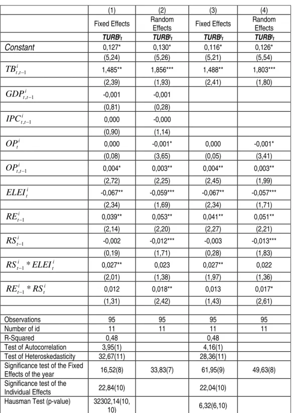
4.2.1. Results
The result of the estimations of equation (2) can be seen in the following table:
Insert table 3 here
There are some differences in the results for the sample of Latin American countries
from those for OECD countries. We shall focus our comparison on estimate (3) because the
Hausman49 test indicated that the best presentation of the results would be with fixed effects, and
the inclusion of the non-significant variables would reduce the efficiency of the significant ones.
Beginning with the economic variables, we can see the change in tax burden in terms of
GDP ( i t t
TB,−1) and the change in the degree of openness in the economy ( i t t
OP,−1) were
significant and with the expected signs.
In the same way as in the OECD countries, the change in tax burden was the variable
the tax burden relative to GDP led to a change in tax structure of 0,01488 (this effect is more
than double the one found in OECD countries).
On the other hand, the change in the level of openness of the economy was significant
and explains changes in the tax structure only for Latin American countries. An explanation for
this result lies perhaps in the long period that these countries went through with a low level of
commercial openness, until the mid-eighties. Even after this period, the level of openness
remained low. Comparing the level of openness during the nineties in Latin American countries
with the average degree of openness of the twenty countries taking part in the initial sample of
Ashworth and Heyndels (2002) between 1965-1995, we find a big difference. For OECD
countries the average was around 73% (data from World Development Indicators, 2003); for
Latin American countries the average was around 51% (see table A.1.1 in Appendix 1). Even
remaining low by the standards of OECD countries, the absolute change in the level of openness
provoked changes in tax structure: when the economy was opened up to make it more
competitive the tax structure was adapted. The inflation rate was not significant. 50.
Moving on to an analysis of the results of the political variables, the main thrust of our
study, two of them proved to be significant enough to explain changes in tax structure: elections
( i
t
ELEI ) and a change in the ideological regime ( i t
RE−1). Elections gave a negative sign and
the change in ideological regime a positive one.
Because of the coefficient sign associated with the variable representing elections we
reach the conclusion that, similar to what happens in OECD countries, there was an attempt to
reduce tax changes in election years, reflecting the pre-electoral moment.51 The reason for this,
as was shown in literature, is the fact that politicians are not prepared to bear the cost that a tax
change represents. Politicians did not make changes in tax structure in election years. In the
positive effect and the significance of the interaction between fragmentation of power and the
election ( i
t i
t ELEI
RS −1* ) in this same estimate. However, as a result of the relative size of the
coefficients of these variables, our results indicated that inertia would still prevail, as in OECD
countries. 52 From the construction of the variable representing the fragmentation of government
- zero if the same party controls the Executive and Legislative branches and one otherwise - if
there is no dispersion of power, there is no doubt that inertia will predominate. On the other
hand, if there is dispersion of power, inertia in relation to the structure of taxes will be weakened
but not reversed because the coefficient of interaction (0,027) is not greater than the coefficient
of the election in isolation (0,067).
From the results found it seems to us that a change in ideological regime has led to
changes in tax structure. 53. As our variable is a dummy that reflects a change in ideology at the
time of the election the only possible interpretation is that a new government (including in terms
of ideology) imposed its tax choice immediately after the election. Our hypothesis was that up
until the election the existing basket of taxes reflects the choice of the government in power.
After the election, if there is an ideological change accompanied by a change in the tax structure,
it will be proof of a choice of tax. So, at least as far as the tax dimension is concerned, we have
removed the possibility that ideological preferences would not impose a basket of taxes
corresponding to it.
Fragmentation of power was not significant enough in the sample of Latin American
countries to explain changes in tax structure, although in some cases it was significant enough to
explain tax changes in OECD countries (given that there were three dummies reflecting
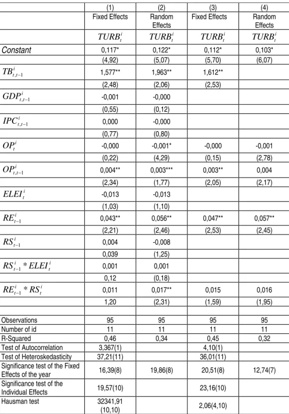
4.2.2. Robustness and sensitivity tests: country effects
In order to analyze if the results above are sensitive to the countries sampled, we
decided to carry out an additional test to check if there is a specific country or group of countries
that were having an effect on the previous results. To do this we carried out a Chow Predictive
test 54 by removing each of the countries in turn and testing if the estimated coefficients were
stable.
Considering all the tests we carried out we ended up concluding that Brazil and
Colombia had a clear effect on the estimated coefficients. 55 Following the result of the Hausman
test the best interpretation of the results would be, once again, the one where fixed effects (the
result in column 3) predominate. Aware of these results we reworked the analysis excluding both
countries and the results are shown in Table 3 below:
Insert table 4 here
All the results presented the same significance level, with the exception of the variable
representing the elections: in isolation ( i t
ELEI ) or interacting with fragmentation
( i
t i
t ELEI
RS −1* ). It stopped being significant at the 10% level. As we do not have a sufficient
number of observations to carry out tests on the two countries, either in isolation or together, we
cannot state whether this result is restricted to a single country or to both of them jointly.
From our main investigation, we can be certain that the ideological change at election
time is not an effect restricted to just some of the countries in the sample. It is valid for all of
them. Tax choice based on ideological preference is the most significant result we found in this
work. We can therefore reject the possibility that tax choice does not reflect ideological
preference in the Latin American countries sampled. The same economic variables showed
5. Main conclusions
The objective of this work was to verify whether ideological changes occurring at election
time defined tax structure changes in Latin American countries during the nineties. This issue
arises because the theoretical literature indicates that the choice of voters is no longer based on
ideological issues in Latin American countries and empirical studies show that this type of
change no longer influences the tax choice in OECD countries.
Our most significant result highlights that changes in the ideology of governments at the
time of elections cause changes in tax structure the following year. After the election, there was
an ideological change accompanied by a change in the tax structure: an ideological choice of
tax. This clearly reflects the predominance of ideological choices when it comes to making tax
choices
In terms of economic aspects two variables also affected tax structure: change in total tax
burden and change in the degree of openness in the economy. In OECD countries the economic
variables that provoked changes on tax structure were both total tax burden and inflation. Maybe
changes in the openness of the economy are much more important to Latin American countries
than to OECD countries because of their history: on several occasions these countries adopted
development policies where a policy of closed commerce was fundamental. With the process of
economic opening, which they underwent, they were obliged to adapt the tax structure of these
countries to the new reality of their commercial partners.
References
Alesina, A. Cohen, G.D. and Roubini, N. (1992) Macroeconomics policy and elections in OECD democracies. Economics and Politics 5: 1-30.
Além, C. and Giambiagi, F. (1999). Finanças públicas: teoria e prática no Brasil. Editora Campus.
Arellano, M. and Bond, S. (1991) Some Tests of Specification for Panel Data: Monte Carlo Evidence and an Application to Employment Equations. The Review of Economic Studies, Volume 58, Issue 2 April, 277-297.
Arvate,P.R., Lucinda, C.R. and Schneider, F. (2004). Shadow Economies in Latin America: what do we know? A highlight on Brazil. Working paper GV/Pesquisa. FGV/EESP and EAESP.
Ashworth, J. and Heyndels, B. (2002) Tax structure turbulence in OECD countries. Public Choice 111: 347-376.
Amorim Neto, O. and Borsani, H. (2004). Presidents and cabinets: the political determinants of fiscal Behavior in Latin American. Studies in Comparative International Development. Vol 39 n01 pp 3-27.
Beck,T.,Clark,G.,Groff,A.,and Keefer,P. and Walsh,P.,2000. New tools and tests in comparative political economy: the database of political institutions. World Bank Working Papers Series n.2283
Beck,T.,Clark,G.,Groff,A.,and Keefer,P. and Walsh,P.,2001. New tools and tests in comparative political economy: the database of political institutions. World Bank Economic Review 15:165-176.
Beck, N. and Katz, J. N., 1995 (1995) What To Do (and Not To Do) with Time Series and Cross-Section Data. American Political Science Review, 89, 634-647.
Baltagi, B. H. (1995). Econometric Analysis of Panel Data. John Wiley and Sons, N.Y.
Barro, R. (1979). On the determinants of public debt. Journal of Political Economy 87.
Baumann, R. (2000). O Brasil nos anos 1990: uma economia em transição. In Baumann, R. (Ed). Brasil: uma década de transição. Edição CEPAL - Editora Campus.
Biglaiser, G. and Brown, D. S. (2003) The determinants of privatization in Latin América. Political Research Quartely, vol 56, no.1, pp 77-89.
Botelho, R. (2002) Determinantes do comportamento fiscal dos estados brasileiros. Dissertação de mestrado apresentada na Universidade de São Paulo.
Bresser-Pereira, L.C. org (1991). Populismo Econômico – Ortodoxia, Desenvolvimentismo e populismo na América Latina. Editora Nobel.
Dornbush, R. and Edwards, S. (1989) Macroeconomic populism in Latin America. NBER Working Paper Series, 2986.
Frieden,J., Ghezzi, P. and Stein, E. (2000). Politics and Exchange Rates in Latin American. Inter-American Development Bank. Research Network Working Paper r-421.
Greene, W. H. (1997) Econometric Analysis – 3rd Edition. Prentice-Hall. Upper Saddle River, N.J.
Gordon, R.J.(1989) Political and economic determinants of budget deficits in the industrial democracies. European Economic Review 33: 934-938.
Hettich, W. and Winer, S. (1997) The political economy of taxation. In C. Muller (Ed), Perspectives on Public Choice, 481-505. Cambridge: Cambridge University Press.
Hettich, W. and Winer, S. (1999) Democratic choice and taxation: a theoretical and empirical analysis. Cambridge: Cambridge University Press.
Hibbs, D. A. (1977). Political Parties and Macroeconomic Policy. American Political Science Review, 71.
Hymer, S. and Pashigian, P. (1962). Turnover of firms as a measure of market behavior. The Review of Economics and Statistics 44:82-87.
Knight, A. (1998) Populism and Neo-Populism in Latin America, especially Mexico. Journal of Latin American Studies, vol.30,number 2.
Kaufman, R. R. and Ubiergo, A.S.(2001). Globalization, Domestic Politics, and Social Spending in Latin America: A time-series cross – sections analysis 1973-97. World Politics, 53, pp 553-87.
Kontopoulos, Y. and Perotti, R. (1998) Government Fragmentation and fiscal outcomes: evidence on OECD countries. In Poterba e Hagen. Fiscal institutions and fiscal performance. Chicago Press.
Lima Jr, Olavo Brasil de (1997). O Sistema Partidário Brasileiro. FGV Editora.
Mankiw, N.G.(1987). The optimal collection of seignorage, theory and evidence. Journal of Monetary economics.
Messere,K. (1993). Tax policy in OECD countries. Amsterdam:IBFD Publications BV.
Perotti, R. and Kontopoulos, Y. (1999) Government Fragmentation and fiscal policy outcomes: evidence from OECD countries. In J.M. Poterba and J. Von Hagen (eds) Fiscal institutions and fiscal performance, 81-102. Chicago Press.
Rae, Douglas (1971). The political consequences of electoral laws. New Haven:Yale University Press, Second edition.
Rodrik, D. (1998) Why do more open government have bigger governments? Journal of Political Economy 106:997-1032.
Rogoff,K. (1990) Equilibrium political budget cycles. American Economic Review 80: 21-36.
Roubini, N. and Sachs, J. (1989). Political and Economic determinants of budget deficits in the industrialized democracies. European Economic Review 33:903-933.
Roberts, K. M. (1995). Neoliberalism and the transformation of Populism in Latin America. The Peruvuian Case. World Politics, 48.
Roberts,K.M. and Wibbels, E. (1999). Party System and Electoral Volatility in Latin America: A test of Economic, Institutional, and Structural Explanations”. American Political Science Review, 93 number 3.
Sabatinio, C. (2002). The decline of ideology and the rise of “quality of politics” parties in Latin America. World Affairs.
Sachs, J. (1989) Social Conflict and Populist Policies in Latin American. NBER Working Paper, March.
Steinmo,S. (1993) Taxation and democracy. New Haven: Yale University Press.
Tufte, E.R. (1978) The political Control of the economy. Princenton, Princenton University Press.
Volkerink, B. and De Haan, J. (1999) Political and institucional determinants of the tax mix: An empirical investigation for OECD countries. SOM research report 99E5.
Wibbels, E. and Arce, M. (2003) Globalization, Taxation, and Burden-Shifting in Latin America. International Organization 57, pp 111-136.
Willianson, J. (1999) What should the bank think about the Washington Consensus. World Development Report, 200.
Widmalm, F. (2001) Tax structure and growth: are some taxes better than others? Public Choice vol 107, number 3-4: 199-219.
Woolridge, J. M. (2002) Econometric Analysis of Cross Section and Panel Data. Cambridge: MIT Press.
Varsano, R. (1997) A evolução do sistema tributário brasileiro ao longo do século: anotações e reflexões para futuras reformas. Pesquisa e Planejamento Econômico, vol 27, n.1.
Tanzi,V. and Zee, H. H. (2000). Tax policy for emerging markets: developing countries. National Tax Journal, vol 53 no.2, pp 299-322.
Figures inside the text
Chart 1: Turbulence index for selected Latin American countries in the 1990s.
0,00 0,02 0,04 0,06 0,08 0,10 0,12 0,14
Chart 2: Average Tax Turbulence – Latin American countries in the 1990s
0,00 0,02 0,04 0,06 0,08 0,10 0,12 0,14 0,16 0,18 0,20
Arg enti ne
Boli
via Brazil Chile Colomb ia
Cos ta Rica
El Salv ado r
Gua tem ala
Mex ico Nicaragu
a Pan ama
Per u Paragu
ay Uru gua y
Table 1. Determinants of Latin American changes on tax structure
Year t E - 2 t E - 1 E t E + 1 t E + 2
Change in tax burden (absolute value) + + + + +
Economic variables
GDP growth (absolute value) + + + + +
Inflation (absolute value) + or – + or – + or – + or – + or –
Openness (level) - - -
Change in openness (absolute value) + + + + +
Political variables
Electoral Manipulation + or –
Ideological change + or -
Dispersion of power - - -
Table 2: Description of the variables used in the estimation
Factor Code Definition Source
Tax Burden i
t t
TB,−1 Variation in total government tax collection,
year on year, in absolute terms for each country (it does not matter if the variation is positive or negative)
Government Finance Statistics Yearbook (several years).
Consumer Price Index i t t
IPC,−1 Variation in the consumer price index, year on
year, in absolute terms for each country
World Development Indicators 2003
Growth of GDP i
t t
GDP,−1 Variation in the rate of GDP growth, year on
year, in absolute terms for each country
World Development Indicators 2003
Openness of the Economy
i t
OP Sum of Exports and Imports as a percentage
of GDP for each year
World Development Indicators 2003
Change in the Openness of the Economy
i t t
OP,−1 Variation of the degree of openness in the
economy, year on year, in absolute terms
World Development Indicators 2003
Election i
t
ELEI Dummy variable with the value one when it is
a presidential election year and zero otherwise
Political Database of Americas (Georgetown University)
Regime
(Ideological Changes)
i t
RE−1 Dummy variable with the value one when
there is an ideological change to the left or to the right in the head of the Executive ; zero otherwise
Beck, Clark, Groff, Keefer and Walsh (2000, 2001)
Fragmentation of Government
(Dispersion of power)
i t
RS −1 Dummy variable with the value zero when the
same party is in control of the Executive and the Legislative branches (Roubini-Sachs’ index 0) and with the value one when there are different parties controlling the Executive and the Legislative branches (Roubini-Sachs’ index 1).
Table 3: Panel estimation of tax turbulence 1991-1999
(1) (2) (3) (4)
Fixed Effects Random
Effects Fixed Effects
Random Effects
TURBit TURBit TURBit TURBit
Constant 0,127* 0,130* 0,116* 0,126*
(5,24) (5,26) (5,21) (5,54)
i t t
TB,−1 1,485** 1,856*** 1,488** 1,803***
(2,39) (1,93) (2,41) (1,80)
i t t
GDP,−1 -0,001 -0,001
(0,81) (0,28)
i t t
IPC,−1 0,000 -0,000
(0,90) (1,14)
i t
OP 0,000 -0,001* 0,000 -0,001*
(0,08) (3,65) (0,05) (3,41)
i t t
OP,−1 0,004* 0,003** 0,004** 0,003**
(2,72) (2,25) (2,45) (1,99)
i t
ELEI -0,067** -0,059*** -0,067** -0,057***
(2,34) (1,69) (2,34) (1,71)
i t
RE−1 0,039** 0,053** 0,041** 0,051**
(2,14) (2,20) (2,27) (2,21)
i t
RS−1 -0,002 -0,012*** -0,003 -0,013***
(0,19) (1,71) (0,28) (1,83)
i t i
t ELEI
RS −1* 0,027** 0,023 0,027** 0,022
(2,01) (1,38) (1,97) (1,36)
i t i
t RS
RE−1* 0,012 0,018** 0,013 0,017*
(1,31) (2,42) (1,43) (2,61)
Observations 95 95 95 95
Number of id 11 11 11 11
R-Squared 0,48 0,48
Test of Autocorrelation 3,95(1) 4,16(1)
Test of Heteroskedasticity 32,67(11) 28,36(11) Significance test of the Fixed
Effects of the year 16,52(8) 33,83(7) 61,95(9) 49,63(8)
Significance test of the
Individual Effects 22,84(10) 22,04(10)
Hausman Test (p-value) 32302,14(10,
10) 6,32(6,10)
Note: z statistics in parentheses. The critical values of the table can be found in parentheses in the table.
Table 4: Panel estimation with Brazil and Colombia exclusion
(1) (2) (3) (4) Fixed Effects Random
Effects
Fixed Effects Random Effects
i t
TURB TURBti TURBti TURBti
Constant 0,117* 0,122* 0,112* 0,103*
(4,92) (5,07) (5,70) (6,07)
i t t
TB,−1 1,577** 1,963** 1,612**
(2,48) (2,06) (2,53)
i t t
GDP,−1 -0,001 -0,000
(0,55) (0,12)
i t t
IPC,−1 0,000 -0,000
(0,77) (0,80)
i t
OP -0,000 -0,001* -0,000 -0,001
(0,22) (4,29) (0,15) (2,78)
i t t
OP,−1 0,004** 0,003*** 0,003** 0,004
(2,34) (1,77) (2,05) (2,17)
i t
ELEI -0,013 -0,013
(1,03) (1,10)
i t
RE−1 0,043** 0,056** 0,047** 0,057**
(2,21) (2,46) (2,53) (2,45)
i t
RS −1 0,004 -0,008
0,039 (1,25)
i t i
t ELEI
RS −1* 0,001 0,001
0,12 (0,18)
i t i
t RS
RE−1* 0,011 0,017** 0,015 0,016
1,20 (2,31) (1,59) (1,95)
Observations 95 95 95 95
Number of id 11 11 11 11
R-Squared 0,46 0,34 0,45 0,32
Test of Autocorrelation 3,367(1) 4,10(1)
Test of Heteroskedasticity 37,21(11) 36,01(11)
Significance test of the Fixed
Effects of the year 16,39(8) 19,86(8) 20,51(8) 12,74(7)
Significance test of the
Individual Effects 19,57(10) 23,16(10)
Hausman test 32341,91
(10,10) 2,06(4,10)
Appendix 1
Table A.1.1: The profile of the sample used in the test
TURB TB IPC GDP OP ELEI RS RE
Number of
observations 140 116 140 140 140 140 126 128
Mean 0,09 0,15 223,68 4,11 51,48 0,22 0,63 0,07
Standard
error 0,1 1,61 993,19 4,31 23,5 0,42 0,49 0,26
Minimum 0 -0.08 -1.17 -10.71 13.75 0 0 0
Maximum 0,81 17,35 7485,5 19,65 122,28 1 1 1
Note: Note that the minimum values are not expressed in absolute terms.
∗
The authors would like to thank GV/Pesquisa for their financing as well as for the comments received about previous versions of this article.
1 Professor, São Paulo School of Business Administration and São Paulo School of Economics. E-mail:
[email protected] Address: Av. Nove de Julho, 2029, São Paulo-SP-Brazil. Zip Code: 01313-902. Phone:
55-11-3281-7765. Fax: 55-11-3284-1789.
2 Professor, São Paulo School of Business Administration and São Paulo School of Economics. E-mail:
[email protected]. Address: Av. Nove de Julho, 2029, São Paulo-SP-Brazil. Zip Code: 01313-902. Phone:
55-11-3281-7765. Fax: 55-11-3284-1789.
3 See Sabatini (2002).
4 Arvate, Lucinda and Schneider (2004) showed that in Latin American countries between 1999/2000 the hidden
economy was estimated to be on average 41.5% of official GDP.
5 This position is not unanimous. Wibbles and Arce (2003) showed that strong leftist political parties in Latin
American countries combine with powerful union movements, the government are much more resistant to shifting tax burdens from capital to labor.
6 Ashworth and Heyndels (2002) did not find evidence that this occurred in 18 OECD countries between 1965-1995. 7 The work of Coppedge (1997) on classification of the parties in Latin American countries shows how historically
important the ideological classification of the parties is.
8 This index was found in the work of Ashworth and Heyndels (2002) but it was not really created by the authors.
They brought into the public arena the methodology developed by Hymer and Pashigian (1962) for the industrial organization area for examining changes in the market share of individual companies.
9 “These are grouped under 6 main headings (codes ending ´000´, where the categories are: taxes on income, on
profits and capital gains, on social security contributions, on payroll and workforce, on property, on goods and services and other taxes) and 19 sub headings (ending in ´00´)”. Ashworth and Heyndels, 2002, page 349.
10 It was not possible to reconstruct TURBULENCE 19 for Latin American counties because we did not have data
broken down by tax.
11 We considered this tax with the code ‘000’ plus the inclusion of taxes on international trade and transactions. 12 The following countries have been used: Argentina, Bolivia, Brazil, Chile, Colombia, Costa Rica, El Salvador,
Guatemala, Mexico, Nicaragua, Panama, Peru and Uruguay. The other five countries were dropped due to the lack of enough data to carry out the empirical procedures described below.
13 Ashworth and Heyndels (2002) explained the smoothing of taxes by assuming that the average taxation rate of
any tax i would be given by the tax revenue obtained by this tax (Ri ) divided by its tax base(Bi ). If the marginal cost
of each tax i is given by MCi (Ri/Bi), where MC´i >0, the tax smoothing condition imposes on the i (i = 1....n) taxes that
MCi (Ri/Bi) = ... = MCn (Rn /Bn ) over time.
14 Ashworth and Heyndels (2002) showed that if the rate of growth of the tax base of i taxes (i = 1...n) were equal the
15 Gordon (1989) demonstrated that in conditions of spending uncertainty the total revenue has to change to
accompany the change in the phase of public spending. The possibility of change in the total revenue does not guarantee maintenance of the tax structure over time.
16 Heittch and Winer (1999).
17 We do not know of specific works on the effects of both political and economic variables on tax composition and
structure tax changes on Latin American countries. The literature on the effects of these variables is much more focused on fiscal results and size of government. See Amorim Neto and Borsani (2004). Tanzi and Zee (2000) had illustrated the differences on the tax structures of both OECD and developing countries in two different periods of time (1985-7 and 1995-7), they did not carry out a formal econometric analysis on which variables are held to cause such changes. The present paper aims to go beyond the results presented there by carrying out such analysis for Latin American countries during the nineties.
18 Throughout this section, we will refer to positive effects of a variable as increasing the turbulence of the tax
structure.
19 It does not matter if the movement is positive or negative.
20Generally what is seen in literature is the opposite of this: taxation determining economic growth. We can se a
good example of this in Widmalm (2001)
21 Defined as the following ratio (corporate income tax + employer social security tax revenue / personal income tax
+ employee social security + goods and services tax revenue).
22 Perotti and Kontopoulos (1999) was not found a significant effect coming from inflation on the primary revenue (at
all levels of government) between 1974 and 1983.
23 It is very complicate to imagine a perfect indexing tax system to neutralize the high or hyperinflation. The tax of
changing prices is so high that it will be impossible to build the indexation rule to preserve the tax on real terms.
24 See Dornbusch and Edwards (1989).
25 Rodrik (1998) had already highlighted the effects of openness on the size of governments.
26 “Perhaps the most important peculiarity in trying to think about sectoral interests in Latin American currency policy
is the role of trade policy, and especially the very high levels of trade protection prevailing in most of the region until the middle 1980s. The trade barriers to finished manufactured goods were prohibitive, as they were in much of region from the 1940s until the 1980s, many factures were essentially in non-tradable production.” Frieden, Ghezzi and Stein (2000)
27 Only in election years. In other years the preference of the voters would be followed. 28 Read Roberts (1995) and Knight (1998) on the transformation of populism.
29 The distribution effect via salaries happened when the idea of a nominal devaluation was rejected, given the
inflationary process (the idea prevalent in these countries was that the inflationary impact of the devaluation might fuel inflation even more).
30 See also Bresser Pereira (1991)
31 Expansion was always accompanied by an external crisis. Nominal devaluation of the exchange rate occurred in
the adjustment thereby eliminating the initial distribution gains.
32 Sachs (1989) also understands that a populist policy goes through a deficit financed by inflation. 33 See the description of Dornbusch and Edwards (1989), mainly for Chile.
34 Latin American countries signed up to the so-called Washington Consensus. Among the targets of this consensus
is fiscal discipline. In spite of these countries implanted the rules of consensus on different moments (Brazil was the last country to adopt fiscal discipline in 1994 and to control the inflation), the inflationary financing of the deficit was eliminated. See Williamson(1999).
35 The tax changes in electoral periods to signal possible changes in distribution in the short run to the electors. They
might choose to exchange a tax on income for private individuals for higher corporate taxes. Voters would only perceive the damaging effect of this substitution after the elections.
36 Biglaiser and Brown (2003) pointed out, there exist a period immediately after election called “honeymoon” when
governments are most able to carry out any intended changes. This happens because after the election the political leaders have more room to maneuver politically, because they have no longer time horizons and can blame the previous government for any problems.
37 See also Hibbs (1977) and Tufte (1978) about the ideological influence of parties on public policies.
38 The power of decision of a minority government over taxes would be three times less than in a party coalition. 39 “The first (second, third) equals 1 if the Roubini-Sachs index equals 1 (2,3) and 0 in the other cases”, (page 359) 40 RS1 (1 if the Roubini-Sachs index is 1, zero otherwise), RS2 (1 if the Roubini-Sachs index is 2, zero otherwise)
party majority parliamentary government; or presidential government, with the same party in the executive and legislative branch).
41 The dummy RS2 was negative and significant (it reduced tax movement) to explain TURBULENCE 19 index. 42 Nicaragua, Panama and Paraguay were excluded from the test because of lack of data for the independent
variables.
43 Any Ideological classification of both parties and coalition in Latin American countries will be subject a
controversy. The major problem is the political spectrum presents characteristics beyond the traditional left and right on European countries (see Coppedge, 1997). This is the case of populism, for example. We could classify populism as right-wing (Perus´s Fujimori and Argentina´s Menem are examples – see Kaufman and Ubiergo, 2004) and left-wing. As mentioned, we adopted the classification from Beck, Clark, Groff, Keefer and Walsh (2000, 2001)
44 We chose to build the variable this way because we would like to compare the OECD countries (excluded Mexico)
and Latin American countries in terms of variables and because the variable representative of dispersion of power (more restrictive than the effective number of parties competing, for example) was not our focus in terms of tests of hypothesis. It is a political control variable.
45 As in all countries in our sample there are only presidential regimes we only got to construct Roubini-Sachs’
indices 0 and 1.
46 Techniques to deal with this sort of database can be found in Wooldridge (2002).
47 The correction of these problems was as follows: for the fixed effects models, the Panel Corrected Standard
Errors Estimator of Beck and Katz (1995) was employed. For the Random Effects Models, the Huber/White Robust Covariance Matrix was used. The software in which the estimations were carried out was STATA, version 7.0. 48We chose to keep some results when they were only significant at the 10% level in one of the estimates: fixed and
random effects.
49 Note that the version of the Hausman test used is the robust version in the presence of the autocorrelation and
heteroskedasticity that is present in Wooldrige (2002, p. 291), because group-wise heteroskedasticity and autocorrelation was diagnosed as being present in all models. For this reason the statistic presented there has two values for degrees of freedom, since it is based upon the F distribution.
50 Additional tests were carried out in order to check for the robustness of this result, including one and two period
lagged economic variables. Unfortunately, since these variables reduced the number of degrees of freedom in the estimation, the results were not presented and did not allow us to choose between the hypotheses.
51 We test the effect of election lag. The result is not report but it will not significant.
52 In OECD countries the interaction coefficient was always positive and greater than the negative coefficient of the
election.
53 Another test was carried out in which we included a dummy variable in order to discriminate if the ideological
change was from the left to the right of the political spectrum. A dummy with vale equal 1 if the new government has the same ideology as the old one, 0 otherwise to allow for the effects of changes in government per se with the same dummy of ideological changes. The results – not presented – indicated one does not find a different effect.
54 Greene (1997)
55 Argentina (F-Statistic = 0,424375; p-value=0,916853); Bolivia (F-Statistic = 0,781613; p-value=0,633942);Brasil