!"
#
$
%
&!
&
' &
% (
!"
#
$
%
&!
&
- ! .
!/0
0 ! $!
! !
&-
1
!
' &
% (
% 2 2 & / &/ && !/ %
3 /! % $ !/
! ! )! &! %!!& !/ ! ! 4 5)! & ! $ 0
Inhasz, Juliana.
Term Structure Dynamics and No-Arbitrage under the Taylor Rule / Juliana Inhasz. - 2009.
44 f.
Orientador: Rodrigo De Losso da Silveira Bueno.
Dissertação (mestrado) - Escola de Economia de São Paulo.
1. Taxas de juros. 2. Taxas de juros – Modelos matemáticos. I. Bueno, Rodrigo De Losso da Silveira. II. Dissertação (mestrado) - Escola de Economia de São Paulo. III. Título.
Acknowledgements
Many people were fundamental in the completion of this dream: become a master in Economics. First of all, my family, which provided the necessary conditions for my personal formation, professional and academic.
Elson Pereira dos Santos, by the affection, support and understanding in every moment of our lives.
My friends Gabriel Henrique Orso Reganati, Joelson Oliveira Sampaio, Eduardo Hiramoto, Isabela Travaglia, Luiz Claudio Barcellos and Simone Miyuki Hirakawa.
All my colleagues and friends at Fundação Getulio Vargas: Maúna Baldini, Thaís Innocentini, Felipe Garcia, Fernando Barbi, Ana Lucia Pinto, Vanessa Gonçalves, Patrícia Pinheiro, Pedro Colussi, and Rodrigo Tolentino. In particular, I’d like to thank Ricardo Buscariolli , Wagner Monteiro, Caio Mussolini, Fulvia Hessel, Luciana Yeung Tai, Rubens Morita and Thiago Rodrigues for all the talk and support during these tough times.
My friends at BM&F: Ainira Agibert, Nathalia de Gan Braga and Paula Favaretto.
My friends at FEA/USP: Alexandre Andrade, Claudia Hiromi Oshiro, Fabiano Martinelli, Gilberto Queiroz, Elton Ribeiro and Franco Viscardi.
All the teachers and friends who helped me in the process, especially Pedro Valls, Richard Saito, Claudio Ribeiro Lucinda, Alexandre Damasceno and Lok Sin Hui.
To CAPES, for financial support.
Abstract
The term structure interest rate determination is one of the main subjects of the financial assets management. Considering the great importance of the financial assets for the economic policies conduction it is basic to understand structure is determined. The main purpose of this study is to estimate the term structure of Brazilian interest rates together with short term interest rate. The term structure will be modeled based on a model with an affine structure. The estimation was made considering the inclusion of three latent factors and two macroeconomic variables, through the Bayesian technique of the Monte Carlo Markov Chain (MCMC).
List of Figures
1 The impulse-response function - output growth shock ... 40
2 The impulse-response function – inflation shock ... 41
3 The impulse-response function – first latent factor shock... 42
4 The impulse-response function – second latent factor shock... 43
List of Tables
1 VAR Dynamics – Estimated coefficients of Φ... 35
2 VAR Dynamics – Estimated coefficients of Σ... 35
3 Short term interest rate – Estimated coefficients of δ1... 36
4 Risk Premia – Estimated coefficients of λ1... 36
5 Standard Deviation Yield Curves – Estimated standard deviation ... 36
6 Latent factors – Principal Components Analysis ... 37
7 Correlations between latent factors and macro factors... 37
8 Correlations between latent factors and yields ... 38
9 Standard Taylor Rule – Estimated coefficients ... 38
Contents
1 Introduction 01
2 Affine term structure model 03
2.1 The model ... 03
2.2 Incorporating the Taylor Rule into the model ... 06
2.3 Forward-Looking Taylor Rule... 07
3 Bayesian Theory – The Monte Carlo Markov Chain method 09 3.1 Gibbs Sampler versus Metropolis-Hastings ... 11
4. Data Description 13 5. Estimation Results 13 5.1 The model – Estimated Parameters ... 13
5.2 Latent factors ... 17
5.3 The impulse-response function... 19
5.4 Taylor Rule ... 21
6 Comments and Conclusions 23 7 Appendix 25
7.1 Stochastic discount factor - Derivation... 25
7.2 Affine Model - Derivation ... 28
1
Introduction
The term structure interest rate determination is one of the main subjects of the …nancial
assets management. Considering the great importance of the …nancial assets for the economic
policies conduction, how such the purchase and sale of government bonds in the primary
market, it is basic to understand structure is determined.
Papers such Litterman and Scheinkman (1991) and Dai and Singleton (2000) suggest the
importance of …nancial factors to understand the dynamics of yield curves. Those papers
consider the existence of dynamic factors which determine the risk premia evolution for
diverse maturities of the term structure. Generally, such dynamic factors are represented
by unobserved state variables, summarising all the relevant information that determine the
yield curve movement.
However, under a macro…nancial framework, the yield curve is not determined solely by
…nancial factors. A signi…cant literature, such as Piazzesi (2001), Ang and Piazzesi (2003)
and Diebold et al. (2005) suggest the importance of the macroeconomic factors for
deter-mining mainly the log term yields. Empirical evidence show that changes in macroeconomic
factors, coupled with well de…ned economic policies rules, a¤ect the yield curve dynamics
throughout the time. Ang, Dong and Piazzesi (2005), using U.S. data, merge the two
frame-works, and estimate a interest rate term structure model with a time-varying risk premia
and no-arbitrage. They consider simultaneously macroeconomic variable and latent factors,
besides specifying the Taylor rule determining the short term interest rate.
In Brazil, the term structure behaves inversely to the one observed in the USA, with
high values for the short term interest rate, and low values for the long term interest rate.
We are, then, lead to the some questions. Can we claim that ADP’s results hold when the
term structure is inversely inclined? What are the main di¤erences? Such questions are
important because they concern mainly developing economies, which are supposed to have a
long term structure lower than the short term. ADP (2005) points out that, only one latent
rate term structure in the same way that ADP (2005), do considering, however, three latent
factors. For this, we use the Monte Carlo Markov Chain econometric method, hereinafter
MCMC, with Brazilian data.
The ADP (2005) model can be considered the most comprehensive, since it develops an
a¢ne model of term structure with time-varying risk premia, and also it considers the
im-portance of interaction between macroeconomic variables and latent factors for determining
the of yield curve movements. Their model is based on Du¢e and Kan (1996) and the
mon-etary policy rule, as the Taylor Rule, is one of its arguments for determining the short-term
interest rate. This type of joint short and long-term interest rate modeling should provide
more information about the dynamic interaction of rates for di¤erent periods.
Only a few papers already had Brazil as focus, such as Matsumura and Moreira (2007),
hereinafter MM, and Shousha (2005). These papers use only one latent factor, and maturities
of 12 months at most. Besides using three latent factors, we opt to use maturities of up to
60 months, with intention to extend the information horizon. The inclusion of two latent
variable, by itself, shows signi…cant contribution to understand the yield curve dynamics,
catching e¤ect not explicit in the macroeconomic factors and not caught by only one latent
factor. Moreover, these papers present, in short-term, consistent results with ADP (2005),
and inverse direction results in long-term, with bigger forecast errors in longer yields. This
paper, however, presents results in inverse direction to those found ADP (2005).
Thus, the inclusion of the two latent variables produces singular results, with positive
variations of the curves given in‡ation shocks and the …rst and the third latent factors, and
negative variations resulting of output shocks and the second latent factor.
The remainder of the paper is organized as follows. Section 2 describes the theoretical
model, considering an a¢ne term structure model and a Taylor rule. Section 3 presents the
econometric method used in this paper. In Section 4, we describe the dataset. Section 5
2
A¢ne term structure model
In this section, we present the main hypotheses of the term structure estimation model:
a¢ne models. This family of models, introduced by Du¢e and Kan (1996), enables one
to specify a time-varying risk premia, accommodating state variables with averages and
covariances also varying over time.
The term structure can be understood as the perception of agents abouth the future
state of the economy, there our paper proposes to draw up a model capturing the dynamic
of interest rate curves, and taking into account the short-term interest rate explained by a
composition of latent factors and macroeconomic variables.
Preliminarly, the interaction between the perception of future economic growth and
macroeconomic variables provides the monetary authorities with important information for
their policy decisions and for the forecasts of market participants in a manner that is
some-what dynamic and recursive: policy decisions today are likely to impact the actions of market
participants today, in‡uencing the interest rate curve in the following periods, which in turn
will in‡uence the decision of the monetary authorities, and so on and so forth.
Furthermore, the use of data with many more maturities makes it possible to extract
more abundant and more accurate information, because long term interest rates re‡ect the
expectations of agents on the spot rate at the long term.
In addition, our paper introduces a non parametric estimation method based on the
Monte Carlo Markov Chain. In this literature, the method, according to ADP (2005),
presents better results than parametric methods, which in Brazil cannot be reasonable,
given the existence of extreme values.
2.1
The model
Following the model developed and used by Ang, Dong and Piazzesi (2005), let us indicate
Xt = gt t ftu | |
(1)
where:
gt is the growth rate of GDP between the periodst 1and t;
t represents the in‡ation rate between the periods t 1 and t; fu
t is a latent variables vector of the term structure of the interest rate;
| means transpose.
Assuming that each variable follows an order 1 autoregressive-type process VAR(1), then
we have:
Xt = + Xt 1+ "t (2)
where
is the coe¢cient matrix of VAR(1);
is the standard deviation matrix;
vector "t i:i:d:N(0;1):
Within this type of model speci…cation, the short-term interest rate can be modeled in
di¤erent ways. In a less sophisticated version and in a generalized way, we can de…ne it as:
rt = 0+ |1Xt: (3)
Substituting the last formula into the vector, as we have seen previously, we have:
rt = 0+ 1;ggt+ 1; t+ |1;uf u
t : (4)
The introduction of alternative forms of the Taylor Rule into the model will immediately
modify equation 4. More structured Taylor Rules impose greater complexity in determining
the short-term interest rate, altering the functional form of equations 3 and 4.
In our model, we can specify the pricing kernel as being an exponential function dependent
on short-term interest rates (rt), the variable risk premia over time( |
t t), and the random component ( |
t"t 1). Thus:
Mt+1 = exp rt
1 2
|
t t+ |t"t 1 (5)
As the time-varying risk premia (given the previously expressed hypotheses), it can be
determined in the following way:
t= 0+ |1Xt (6)
where 0 is a scalar.
From the pricing kernel we can …nd the stochastic discount factor mt+11 :
mt+1 = logMt+1 = 0+ |1Xt+1 (7)
where 0 is a scalar and 1 is a vector of dimension identical to Xt+1.
With the set of instruments developed so far, it is possible to derive the expression for
the term structure of an a¢ne model. For this, it is necessary to …nd an expression which
de…nes the yield of a zero-coupon bond maturing in any periodn. Thus, denotesyt(n) as the
term structure we wish to …nd with these characteristics, we have:
Pt(n) = exp ny
(n)
t (8)
And therefore:
yt(n) = logP
(n)
t
n =
p(tn)
n (9)
where
Pt(n) is the price of the asset in period t; n is the price of the asset in period;
p(tn) is the logarithm of the asset price levels in period t.
In this model, the price of a bond is necessarily related with exponential function of the
state variables contained therein. In algebraic terms:
Pt(n) = exp (An+Bn|Xt) (10)
The equations exhibited so far, especially the algebraic speci…cation of the vector Xt and
the pricing kernel in its usual form enable us to develop a related term structure model.
Thus we know that:
yt(n)=an+b|nXt (11)
where:
an is a scalar determined by An
n ;
bn is a vector of dimension j 1 given by Bn
n : 2
2.2
Incorporating the Taylor Rule into the model
Since the model estimates the term structure of the Brazilian interest rates is according
with the existence of a variable risk premia over time, the short-term interest rate must also
align itself with those objectives. That is done by introducing the rule for determining the
short-term interest rate, namely the Taylor Rule, which will substitute the basic rule shown
in the model by the equations 3 and 4.
The Taylor Rule (1993) presented in its classic version, captures the responses of the
monetary authority (in the Brazilian case, the central bank) to movements, desirable or
oth-erwise, of relevant macroeconomic variables (usually, in‡ation and output). These responses
are given by variations in the basic short-term interest rate.
Although they present a satisfactory description of the behavior of the term structure,
the models which use latent factors do not provide su¢cient information about the economic
nature of interest rate shocks and therefore become less relevant for an analysis of the term
structure dynamics. This information will, therefore, be provided by the rule for determining
short-term interest rates highly in‡uenced by macroeconomic factors.
According to ADP (2005), any version of the Taylor rule will be compatible with the
structure of the model, provided the latter belongs to the class of related models. Several
versions of the Taylor Rule exist, but we estimated on the forward-looking type of Taylor
Rule.
2.3
Forward-Looking Taylor Rule
In the case of the Forward-Looking Taylor Rule, we assume the central bank adjusts
interest rates according with the expectations of real GDP growth and in‡ation in the coming
periods.
In the event the central bank considers only those elements within a …nite horizon, we
have a Forward-Looking Taylor Rule whose algebraic form is given below:
rt= 0+ 1;gEt(gt+1) + 1; Et( t+1) +"t (12)
where rt is the short-term interest rate, Et(gt+1) is the expected real GDP growth at
periodt+ 1(or the expected output growth in the period), Et( t+1)is the expected in‡ation
Rewriting the equation in its vector form, we have:
rt = 0+ 1;g 1; 0 Et(Xt+1) +"t (13)
= 0+ 1;g 1; 0 ( + Xt) +"t
= 0+ 1;ge1+ 1; e2
|
+ 1;ge1+ 1; e2
|
Xt+"t (14)
where ei is a vector of zeros, except in the ith position, where it is equal to one.
Re-writing equation 13 according to the speci…cations of a related structure model, we
have:
rt= 0+
|
1Xt (15)
0 = 0+ 1;ge1+ 1; e2
|
(16)
1 = | 1;ge1+ 1; e2 + 1;ue3 (17)
"t = 1;ufut (18)
with
1;u = 1;u (19)
The same can be done considering an in…nite horizon, that is, in the event the central
bank considers the entire future path of the relevant macroeconomic variables for a rate .
rt= 0+ 1;g bgt+ 1; bt+"t (20) Where: b gt= 1 e |
1(I )
1
+e|
1(I )
1
Xt (21)
and
bt=
1 e
|
2(I )
1
+e|
2(I )
1
Xt (22)
3
Bayesian Theory – The Monte Carlo Markov Chain
method
A brief description of the econometric methods is given here. All the methodology is
based on that used by Du¢e and Kan (1996) and ADP (2005).
Estimating the model of the interest rate term structure is done using the Bayesian
technique of the Monte Carlo Markov Chain (MCMC).
Bayesian econometrics can be summarized as the systematic result of probability theory:
the Bayes theorem, which the immediate relationship between the conditional probability of
A given B and the conditional probability of B given A can be found. In algebraic terms:
P (AjB) =P (BjA) P (A) P(B) 1 (23)
The distribution of A given B is the principal aim rule in econometric analysis, since it
the model. Of the exist methods for extracting a sample from a given distribution , we
have used the MCMC method when the methods of available distribution, actually available
distribution and distortion or transformation of samples from a standard distribution are
not applicable. In this case, we can simulate a stochastic process until its results derive from
stationary distribution (which the distribution we are seeking) and, based on this sample,
we make the statistical inferences.
Thus:
P( jy) = P(yj ) P( ) P(y) 1 (24)
where P (yj ) is the probability of the model, P( ) is the prior distribuition of the parameter and P (y)is the marginal distribuition of the sample.
The MCMC is a method of sampling the target distribution by constructing a Markov
chain in such manner that the stationary distribution of simulated chain is exactly the
target distribution we are looking for. There are two ways of building a chain whose aim
is a stationary target distribution: the Metropolis-Hastings algorithm and Gibbs sampling.
The advantages and disadvantages of each one are explored in the following subsection. Let
us say in advance, the algorithm used in this study will be the Metropolis-Hastings.
Therefore application of the MCMC is done by simulating a random process until its
results derive from a stationary distribution (this is the distribution we are looking for) and
from this sample it is possible to make statistical inferences regarding the parameters. After
subsequent distributions are found, the results can be summarized by calculating the values
expected and the variances of the distribution found for each parameter, as follows:
E( kjy) =
Z
kp( jy)d (25)
V ar( kjy) =
Z
2
There are many reasons for justifying the use of the MCMC method in this estimate. One
of the advantages of this method is the fact that it doesn’t presume a numerical maximization
methodology, while the validity of the methodology employed can be veri…ed using Markov
chain convergence. So we can simulate a random process in such manner that results derive
from a stationary distribution, and as a result, it is possible to use this sample to make the
necessary statistical inferences.
In addition, this method allows us to consider that one or more yields have been observed
with measurement errors (ADP, 2005). It is also important to consider that the Bayesian
estimate method provides a subsequent distribution of a part of the time vector , which
latent variables are speci…ed, and in this way we can obtain a good estimate of the monetary
e¤ect policy shocks. In addition, it is applicable to non linear and high dimension models.
Thus the use of the MCMC estimate produces better results regarding the soundness and
the quality of the inference made.
3.1
Gibbs Sampler versus Metropolis-Hastings
As already mentioned, there are two ways in which we can …nd the Markov Chain, so
that, by de…ning the a priori distribution, it is possible to …nd the stationary distribution
associated with it. These are the Gibbs Sampling and the Metropolis-Hastings algorithm. In
both cases we have to know the a posteriori probability density function to the …rst constant,
that is,
P ( jy)/P (yj ) P( ) (27)
The Metropolis-Hastings algorithm uses the idea of rejection methods, so that a value is
generated from an auxiliary distribution and accepted as a given probability. Thus it ensures
that the convergence of the chain to the equilibrium distribution is therefore the a posteriori
Using this algorithm is not conditional on knowing the distributions of the parameters,
doesn’t require such distributions to be of the complete conditional type. Intuitively, this
algorithm “decomposes” the unknown conditional distribution into two parts: a known
dis-tribution, which generates “eligible” points, and an unknown part from which the simulation
acceptable criteria. Which ensure the algorithm with a correct equilibrium distribution.
The Metropolis-Hastings algorithm signi…cantly increases the number of applications that
can be analyzed, without the conditional density of the parameters being necessarily in a
closed form.
All this leads us to conclude that by using the Metropolis-Hastings algorithm, the chain
can remain in the same state for many iterations (EHLERS, 2007). Therefore it is convenient
to monitor the time during the iterations remain in the same state, by using the average
percentage of iterations for new acceptable values. It is worth pointing out that although it
is possible to choose the proposed distribution in an arbitrary manner, choosing it ensures
the algorithm e¢ciency.
Gibbs sampling is a special case of the Metropolis-Hastings algorithm in which the
pa-rameter vector elements are updated one at a time.
In the case of Gibbs sampling, the chain always moves to a new value, so do not exist
acceptance-rejection mechanism of value, as in the case of the Metropolis-Hastings algorithm.
Thus the transitions from one state to another occur according to the complete conditional
distributions. For this to occur, the parameters of the model must have a closed form, that
is, their distributions are known.
In many situations, the generation of a sample directly from the probabilities of the
para-meters can be complicated and even impossible, which at times makes it impossible to apply
Gibbs sampling. So that justi…es the option for the Metropolis-Hastings algorithm, given the
modeling of the problem using latent variables as an argument, it is not possible to generate
a sample using direct probabilities of the parameters, nor can we ensure speci…c distributions
for each parameter. In this case we have to use the Metropolis-Hastings algorithm in order
4
Data Description
In order to estimate the model, are used macroeconomic variables series and …nancial
se-ries of interest rate curves. In the case of the macroeconomic variables, we use the industrial
production variable as proxy for GDP growth serie. Also we use the expected GDP growth
in the following month, as well as the evolution of the IPCA for the evolution of in‡ationary
expectations and the expectation regarding the evolution of the IPCA. The industrial
pro-duction and IPCA series are the responsibility of the Brazilian Institute of National Statistics
and Geography3. The expected GDP growh series is the responsibility of the Central Bank
of Brazil4. For the data of the term structure, we use the average PRE X DI swap rate for
the 1, 2, 3, 4, 5, 6, 12, 18, 24, 36, 48 and 60 month maturities obtained from the database
of the Mercantile and Futures Exchange (BM&F)5, and are considered on a monthly basis,
from January 2000 to June 2008.
5
Estimation Results
In this section we present the results for the estimated models.
In our estimations, we use 25,000 simulations after a burn-in sample of 5,000. We report
the posterior mean and posterior standard deviation of each parameter, in parentheses. The
sample period is January 2000 to June 2008, with monthly data frequency.
5.1
The model - Estimated Parameters
Tables 1 to 5 show a posterior distribuition of the average values of the parameters,
initiating for the coe¢cients of the VAR, and following for the coe¢cients of the short term
interests rate, for the parameters of the equation that determines the risk premia and for
standards deviation estimated of the errors of term structure observations.
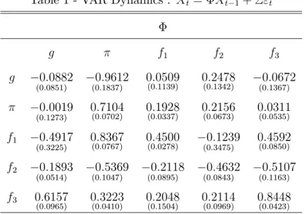
As we can see, regarding to the coe¢cients estimated for the VAR (in Table 1), it has an
inertia in the in‡ation and the third latent factor. The standard deviations of such estimates
are low (respectively, 0.0702 and 0.0423), so that indicates the signi…cance of these variable
in the respective equations. Such results con…rm situations in recent years in our economy,
with persistent in‡ation and periods of relative monetary contraction6.
However, the output growth doesn’t show the same behavior. The estimated coe¢cient,
in this case, is negative, so that indicates an error in trajectory of the economic activity in
the studied period. Moreover, through its a high standard deviation, that the estimation of
this coe¢cient generates a non signi…cant result.
Regarding to the macroeconomic variables, in the equation of output growth, we see
that only coe¢cients related to the in‡ation and the second latent factor are statistically
signi…cant, estimated in -0.9612 and 0.2478 (with standard deviation in 0.1837 and 0.1342,
respectively). The output growth presents negative signal, but it is not statistically
signif-icant. Also we can observe that, as the coe¢cient of the in‡ation in the equation of the
economic growth is negative, variation in the in‡ation is positive, as a consequence, the
economic growth has a reduction.
In the equation of in‡ation in VAR, also we notice that output growth is not statistically
di¤erent of zero, showing not to be signi…cant for the determination of this variable. However,
we see, for the results of the model, the high inertia of the in‡ation, with estimated coe¢cient
in 0.7104. Regarding to the latent factors, we notice the signi…cance of …rst and the third
latent factors, opposing the no signi…cance of the other latent factor in the determination of
the in‡ation.
Regarding the equations of determination of the latent variable, we observe that the
macroeconomic factors are very important for forecast of the same ones. This is observed by
the signi…cance of the coe¢cients of economic growth and in‡ation. Thus, we can conclude
that the macroeconomic variables add important information for the modeling of latent
factors and represent an addition of e¢ciency for the estimation of the term structure.
Also we see that the …rst factor is determined not only by last values, as for the in‡ation
and the third latent factor. The three coe¢cients are statistically signi…cant, and presents
positive signal. The second latent factor presents, in the VAR equation, statistical
signi…-cance for all the coe¢cients. However, all the coe¢cients present negative signal. Finally,
the third latent factor is determined by the two macroeconomic factors (with coe¢cients
of 0.6157 for output growth and 0.3223 for the in‡ation) and by the second latent factor,
beyond being determined by its proper last values. In this case, all estimated coe¢cients
present positive signal, indicating that variations in the others variables generate impact in
the third latent factor, with same signal.
We can see, as Litterman and Scheinkman (1991), that the …rst factor is related directly
to the dynamic of the in‡ation in the period, as well as second factor is related to proxy
of economic growth. Such conclusions evidences in the analysis of the impulse-response
function.
[- insert Table 1 here -]
In Table 2, we have the estimated coe¢cients for the standard deviation matrix of auto
regressive vector (VAR). We can notice that part of the coe¢cients does not present statistic
signi…cance, given that the standard deviation of the estimates is very high. This matrix,
however, is essential to understand as yield curves will react to shocks in the vector state
variables. This is seen in the impulse-response function analysis.
[- insert Table 2 here -]
In the equation of determination of the short term interest rate (Table 3), we observe that
the coe¢cients are signi…cant. The coe¢cient for the GDP growth is negative. Thus, when
the economic growth is above of its potential level, the interest rate increases. Moreover, we
rate, evidencing the great impact of the in‡ation on the short term interest rate. This result
con…rms the current Brazilian economic policy of combat to the in‡ation through in‡ation
target.
We see, also, that the variation in the in‡ation generates a great impact on the short
term interests rate. This can be understood through the dynamic between such variables,
and the short space of time that exists between the moment that occurs the variation of
prices and the adjustment next to the short term interest rate. The same it is not veri…ed
between the short term interest rate and the economic growth, since the adjustment between
such variable is slower.
Moreover, we impose the restriction 1;ui = 1;for i = 1;2;3: This restriction doesn’t
modify the estimated values in the model, since the series of latent factors can be re-scheduled
of arbitrary form.
[- insert Table 3 here -]
In Table 4 we have the estimated coe¢cients for the risk premia. The signi…cance of
these indicates that, really, the risk premia must be considered changeable in time.
Here we see the importance of the macroeconomic variables and latent factors in the
determination of the risk premia variability, since that all the coe¢cients are signi…cant, also
those related to output growth. This result, particularly, opposes to the results evidenced for
ADP (2005), which the output growth isn’t a statistical signi…cant to explain the variation
of the risk premia in time. However, they con…rm the results found by Hui (2006), proving
changeable macroeconomic variables and latent factors are important for determination of a
risk premia variation in the time. Moreover, also we can conclude the excess return changed
signi…cantly in the time.
[- insert Table 4 here -]
structure (in basis point). As we see, the observation standard deviation is fairly large.
Also, standards deviations of the long term interest rates are relatively bigger than those
calculated for the shortest rates. For example, the observation error standard deviation of
the 30 days yield is 0,12 basis point, while the observation error standard deviation of the
1800 days yield is 10 basis point.
This result does not con…rm the theory defended by ADP (2005), which shows that
tradi-tional a¢ne models often produce large observation errors of the short end of the yield curve
relative to other maturities. However, since we are studying the Brazilian term structure, we
know that it presents an inverted pattern. Thus, we must have opposite results: standard
deviation is lower in the vertices of short term and bigger in the vertices of long term. For the
30 days yield, for example, the measurement errors are comparable to, and slightly smaller
than, the estimations containing latent and macro factors. These results were also found in
Hui (2006).
[- insert Table 5 here -]
The di¤erence in the results is justi…ed because of the three latent factors. Many papers
use only one latent factor, and …nd bigger standard deviation in short term. When we use
three latent factors, the observation error in the segment of the yield curve is lower than
with only one latent factor7.
Note that the largest observation error variance occurs at the long end of the yield
curve, which indicates that treating the long rate as an observable factor may lead to large
discrepancies between the true latent factor and the long rate.
5.2
Latent factors
The monetary policy shocks identi…ed using no-arbitrage assumptions depend on the
behavior of the latent factors. In this paper, we use three latent factors as arguments of the
model. Many papers, as Hui (2006) and ADP (2005), use only one latent factor. Although,
Litterman and Scheinkman (1991) opt to the use of three latent factors, with economic
interpretations of level, slope and curvature of the yield curves. An interesting question is
to understand which criteria de…nes the amount of latent factors in a model of yield curves.
The criteria of the number of latent lactors in this model is the Principal Decomposition
Analysis (PCA). The central idea of this method is to …nd, as base in the data of the yield
curves, the implicit factors that a¤ect all the curves (that is, the latent factors) and to
calculate the participation of these in the variance of spreads of yield curves. The results of
the PCA can be seen in Table 6.
[- insert Table 6 here -]
In our model, the …rst latent factor is responsible for 93% of the variance of yield curve
spreads. The second factor totalizes 6% of the variance of curves, accumulating 99.3% of
the total variance. The third latent factor contributes with 0.58% of the total variance of
the curve. The three factors add 99.9% of the total variance of yield curves. The others
factors are responsible for 0.1% of the variance, and they are not considered in the model.
Therefore, three latent factors are considered, corroborating the results of Litterman and
Scheinkman (1991).
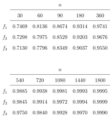
To characterize the relation between latent factors with macro factors and yields, Tables
7 and 8 report correlations of the latent factors with various instruments. Table 7 shows
that the …rst factor is positively correlated with in‡ation at 43.02% and negatively correlated
with output growth at - 68.13%. The same results are shown in other latent factors: the
second latent factor is positively correlated with in‡ation at 43.50% and negatively correlated
with output growth at - 68.09%. Finally, the third latent factor is positively correlated with
in‡ation (at 44.31%) and negatively correlated with output growth (at -67.12%).
[- insert Table 8 here -]
The correlation between …rst latent factor and the yield range is between 74% and 99%;
and for the second latent factor, the correlation range is between 73% and 99%. Finally, the
correlation between third latent factor and the yield range is between 71% and 99%.
Importantly, the correlation between the latent factors and any given yield data series is
not perfect, because we are estimating the latent factors by extracting information from the
entire yield curve, and not just a particular yield. Moreover, we notice that the correlation
increases with maturity. Recalling the results expressed in Table 5, we see that rates of
long-term present prediction errors with standard deviations higher when compared to
short-term rates. Thus, there is greater degree of uncertainty in long rates, which brings the
responsibility of the factors not observed in the understanding of such variations.
5.3
The impulse-response function
We analyze the contribution of each variable of the state vector in the dynamics of the
term structure. So, we intend to see which the impact in each variable of the state vector in
the dynamics of the yield curves. This is made by analysing the impulse-response function.
The …gures are in attached, to the end of the text.
Figures 1-A to 5-A shows the response of yields of 30, 60, 90, 360, 1080 and 1800 days
to a shock in state vector variables. Figures 1-B to 5-B show the response of yields of 30,
60, 90 and 360 days to a shock in state vector variables.
[- insert Figure 1 here -]
[- insert Figure 2 here -]
[- insert Figure 4 here -]
[- insert Figure 5 here -]
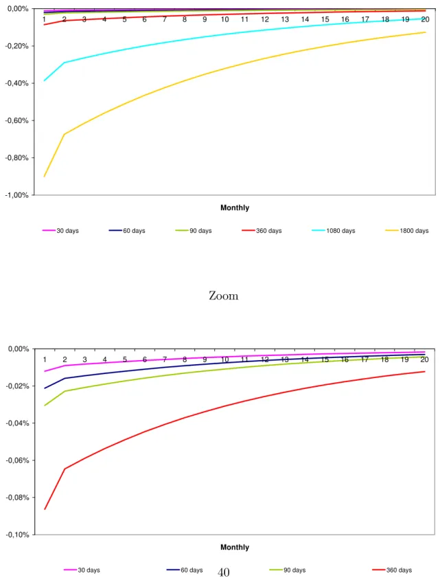
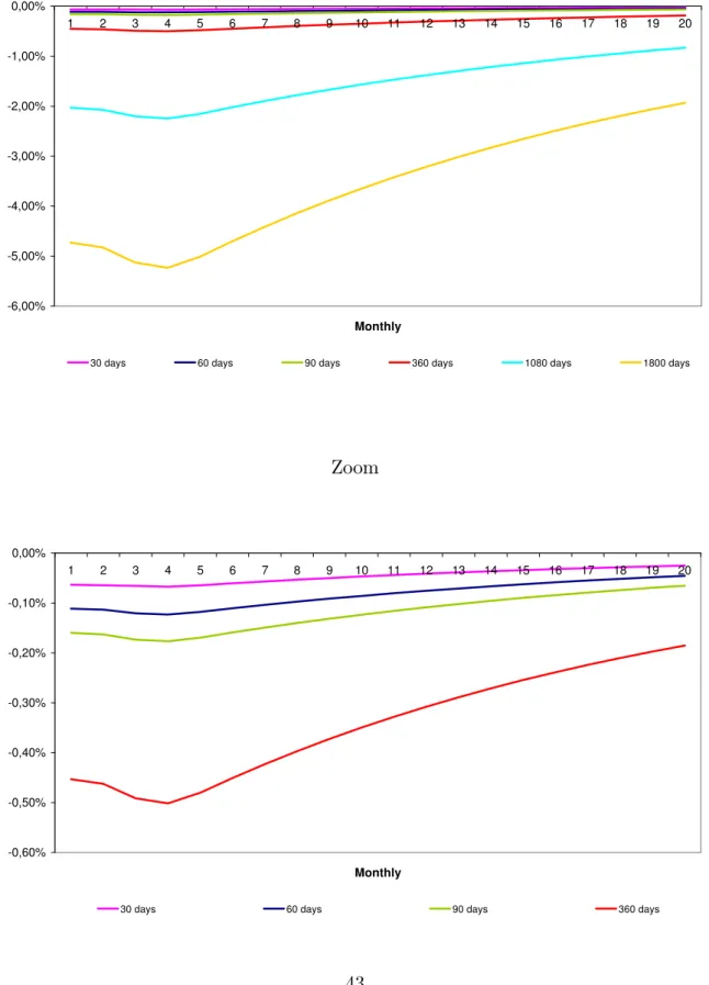
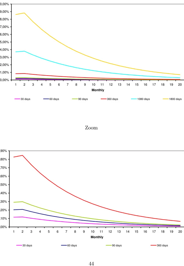
Figure 1 shows the response of yields to a shock in the output growth. Figure 2 shows
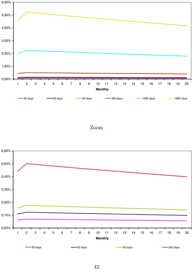
the reply of same yields to a shock in the in‡ation. The Figures 3, 4 and 5 show the reply
of yields to a variation in the …rst, second and third latent factors.
In Figure 1, we can notice a shock in the output growth generates a negative result in
the term structure, moving it down. Since, the estimated coe¢cient for the output growth
in the determination of the short term interest rate is negative, this result is in agreement
with the estimated model.
In Figure 2, we see the e¤ect of a shock in the in‡ation on the yield curves is in accordance
with the waited forecast for the economic theory. A shock in the in‡ation makes with that
all the term structure dislocated for top, in a movement of opening of the curve. Based in
the economic theory, an actual in‡ation is bigger than expected in‡ation in the model, so
that makes the monetary authority increases the short term interests rate, inducing people
recalcuted your expectations of the future interest rate. This movement makes with that all
the long term interest rates modi…ed. First of all, we notice that yiels of bigger maturity
react the variations in the in‡ation tax of more intense form, front to the variations of the
stretch short of the curve. As the forecast horizon if expands, these curves of longer maturity
revert it quickly to the equilibrium and it is faster than in the shorter maturity.
Also we notice, in Figure 2, a great persistence of the in‡ationary shocks in the yield
curves. This result is expected, observing the estimated coe¢cients in the VAR of the state
vector and the estimated coe¢cients for the short term interest rate.
In Figures 3, 4 and 5, we observe the e¤ect of shocks in the latent variable on the yield
curves. The …rst latent factor becomes related to the change in output growth , while second
We conclude similarly by, observing the impulse-response functions of the curves before
variations in the in‡ation and the second latent factor. The third latent factor is understood
as an interaction between the other two, showing a bigger relevance of the changeable
in‡a-tion, making with that a shock in this factor, generating a positive variations in the yield
curves. It is important to stand out that the high inertia of the shocks of the latent factors
in the term structure can be justi…ed by the high coe¢cients found in the auto-regressive
vector.
In all results, we can see the greatest impacts occur in long curves, which contradicts the
results found by ADP (2005). Part of this result can be explained by the behavior of interest
rates in di¤erent markets. In the U.S. market, interest rates for long term are higher than
interest rates for short term. Thus, considering the present value of an asset, the higher the
maturity, the greater the discount on the value of it, the lower their price in present value.
Thus, the impact on these values, in present value, is lower when they have relatively long
maturities than on short-term assets. In Brazil, however, interest rates are behaving in a
contrary pattern: the interest rates for short term are high and interest rates for long term
are lower. Thus it happens the opposite: since long rates are relatively low, when we bring
the value of a particular asset to the present, the discount becomes small, which is re‡ected
in major impacts to the long-term rates.
5.4
Taylor Rule
The models with a¢ne structure accomodate diverse speci…cations of Taylor rules. We
test two types of the Taylor rules: standard Taylor rule, with proxys for in‡ation and
eco-nomic growth in level, and Forward Looking Taylor rule, considering the expectations of
in‡ation and economic growth.
In Table 9, we have the comparison between the stantard Taylor rule determined for the
model and Ordinary Least Squares (OLS). We see the estimated coe¢cient for the economic
theory. However, the papers that use brazilian data, such a type of erratic behavior of the
economic activity in the determination of the short term interest rate is relatively common.
[- insert Table 9 here -]
The estimated coe¢cients for the in‡ationary behavior indicate the relevance of such
variable in the determination of the monetary policy. The estimated value for the coe¢cient
by OLS is high, if it is compared with the estimated coe¢cient through the econometric
model, in 0.801.
Also we can see that the standard-deviation of the estimates for the model are lesser than
estimated by OLS8.
The results of the Forward Looking Taylor rule9 expressed in Table 10 show that in‡ation
has a great importance in the determination ofr, in relation the estimated Taylor rule in the
standard form. The estimation of our model by means of a formulation of standard Taylor
rule generated a coe¢cient for in‡ation of 0.801, whereas with a Forward Looking Taylor
rule, this coe¢cient increases to 1.0084. This type of behavior re‡ects the great concern of
the monetary authority has in the controlling the increase of the price levels.
[- insert Table 10 here -]
Finally, we can notice the estimated coe¢cient for the output growth starts to be
pos-itive, opposing the joined results previously, explicit in Table 10. With that the estimated
coe¢cient for the economic growth was of -0.165, whereas it starts to be of 0.0590.
8The standard Taylor rule estimated OLS makes use only of the short term interests rate, whereas the estimate for the model uses information contained in all the term structure.
6
Comments and Conclusions
To know the term structure and the possible relations with other economic variables is
a very interesting form to understand the macro…nancial dynamics of the economy. Thus,
the main objective of this paper, using all the theoretical knowledge on term structure,
shape the term structure, in set with a well de…ned monetary politics rule. Such monetary
rule is capable of generationg, in singular way, information about the behavior of the term
structure. Moreover, the importance of the macroeconomic variable in the determination of
the yield curves is theoretically known and to including variable macroeconomic, in way to
gain our analysis for the Brazilian case.
We decide to include latent factors believing that they have information about the yield
curves that are not caught by the GDP growth and in‡ation. Many scholars questioned
the possible correlation between the macroeconomic variables and the latent factors, and
the validity of its inclusion in models of this type. Here, the inclusion of these factors in
addition to the macroeconomic variables was made because it has intrinsic factors to the
macroeconomic variables that are not captured by the coe¢cients when we estimated the
term structure. This con…rms the signi…cance of the latent factors in the estimation of the
model. If such factors were not considered, possibly the estimation errors would be extended,
and the estimation would not express of adequate form the term structure.
The estimation of the model is made by the Bayesian technique of Monte Carlo Markov
Chain (MCMC). This technique allows to …nd the posterior distributions of the parameters
of the model, since it is possible to assume a prior distribution. The great advantage of
this method is to allow inferences on the studied parameters, exactly in cases which we do
not obtain analytical solutions. Thus, the MCMC skirt such problem through the use of
an algorithm that simulates markov chains and extracts distributions that the stationary
distribution of the chain is exactly the distribution that we are looking for.
The result are especially interesting since this technique produces di¤erent results from
the problem considering the existence of non observed factors in set with observed variables.
With relation to the results, we can conclude the importance of the macroeconomic
variables in the determination of the brazilian term structure. The yield curve is in‡uenced
for the variation of the macroeconomic variables, by short term interest rate and of the
intrinsic latent factors to the term structure. Shocks in the macroeconomic variables produce
a bigger e¤ect on the short term interest rates, and minors variations on the longer rates.
However, both the types of shocks are important for the evolution of the yield curve, and
7
Appendix
7.1
Stochastic discount factor - Derivation
In this appendix, we describe how to compute the stochastic discount factor.
First, we know that:
Pt(n) =Et Mt+1Xt+1 (A1)
where
Pt is asset price in t;
Mt+1 is the stochastic discount factor;
Xt+1 is the asset payo¤ in t+ 1:
Pt(n)=Et Mt+1Pt(+1n+1) (A2)
Also we know that Pt(n) is the price of zero coupon bond of maturityn at time t. Thus:
Pt(1) =Et(Mt+1) = exp ( rt) (A3)
where rt is risk neutral rate.
We can show that log (Mt+1) is a linear function of the state variables. Therefore:
logMt+1=mt+1 = 0+ |1Xt+1 (A4)
where
0 is scalar and
?
In equation 2 we saw:
Xt+1 = + Xt+ "t+1 (A5)
where
is a constant;
is the estimated coe¢cient matrix of VAR(1);
is the standard deviation matrix of VAR(1);
"t IID N(0; I).
Substituting the equation 2 in equation A4, we have:
mt+1 = 0 + |1( + Xt+ "t+1) =Et(mt+1) + |1 "t+1 (A6)
For assumption, Mt+1 has a lognormal distribuition, thus:
exp ( rt) = exp Et(mt+1) +
1
2var(mt+1) (A7)
However:
var(mt+1) = Et (mt+1 E(mt+1))2 = (A8)
= |
1 vart("t+1) | 1 =
| t t
where
t = | 1 =covt("t+1; mt+1) (A9)
is the risk premia.
exp ( rt) = Et(Mt+1) = (A10)
= exp mt+1 |1 "t+1+
1 2
| t t
Finally, we can conclude that:
mt+1 = rt
1 2
|
7.2
A¢ne Model - Derivation
As we explain in section 2, we denote the jx1vector of state variables as:
Xt = gt t ftu | |
(B1)
where
gt is the output growth from t 1 and t;
t is the in‡ation rate from t 1 and t; fu
t is a vector latente state variable that.
We specify that Xt follows a VAR(1), that is:
Xt = + Xt 1+ "t (B2)
where
is a constant;
is the estimated coe¢cient matrix of VAR(1);
is the standard deviation matrix of VAR(1);
"t IID N(0; I).
The short-term interest rate can be de…ned, in generic form, as:
rt= 0+ 1;ggt+ 1; t+ 1;uf u |
t : (B3)
To complete the model, the price kernel is speci…ed as:
Mt+1 = exp rt
1 2
?
t t+ ?t"t 1 (B4)
t= 0+ |1Xt (B5)
The pricing kernel prices all assets in the economy, which are zero coupon bonds:
Pt(n)=Et Mt+1Pt(+1n 1) (B6)
which Pt(n) is the price of zero coupon bond of maturityn at time t.
We can see the price of zero coupon bond of maturity 0is equal to face value:
Pt(0)+1 = 1 (B7)
Thus,
Pt(1) =Et(Mt+1) (B8)
But, in this type of model, the price of a bond is necessarily an a¢ne exponential function
of the state variables contained therein. In algebraic terms:
Pt(n) = exp (An+B|
nXt) (B9)
Considering these two forms of to see the price of a bond with maturity n, we see that:
Pt(1) =Et(Mt+1) = exp ( rt) = exp ( 0 |1Xt) = exp (A1+B1|Xt) (B10)
Therefore:
Thus:
Pt(n+1) = Et Mt+1Pt(+1n) (B12)
= Et exp rt 1
2
|
t t+ |t"t+1 exp (An+Bn|Xt+1)
= exp rt 1
2
|
t t+An Et[exp (Bn|( + Xt+ "t)) + | t"t+1]
= exp rt 1
2
|
t t+An+B|n +B |
n Xt Et[exp ((B |
n +
|
t)"t+1)]
Considering "t i:i:d:N(0;1), then exp [(B|
n +
|
t)"t+1] lognormal:
Pt(n+1) = exp 0 |1Xtt
1 2
|
t t+An+Bn| +Bn| Xt exp [Et((Bn| + |
t)"t+1)]
(B13)
+ 1
2vart[(B
|
n +
| t)"t+1]
= exp 0 |1Xtt
1 2
|
t t+An+Bn| +B |
n Xt exp [Et((B |
n +
|
t)"t+1)]
+ exp 1 2(B
|
n +
|
t)var("t+1) (Bn| + | t)
|
= exp 0+An+B|n( + 0) +
1 2B
| n
|B n+ [B
|
n( + 1) |1]Xt
Recalling that:
1. exp [( |
t +Bn|) "t+1] has a lognormal distribuition;
2. "t+1 i:i:d:N(0; I) ;
3. B|
n t is a scalar and, therefore, Bn| t= (Bn| t)|= |t |Bn;
Equaling the coe¢cients obtained in the last equality (equation B13) with those
encoun-tered in equation of the bond price in Pt(n+1), we …nd the following equalities, according to
various recursive relations:
Pt(n+1) = exp An+1+Bn|+1Xt (B14)
We have:
An+1 = An+Bn|( + 0) +
1 2B
|
n |Bn 0 (B15)
B|
n+1 = Bn|( + 1) |
1
with An = 0 and Bn = 1:
Another relevant variable to understand the related term structure of interest rate model
is the expectation of the excess holding period return (HPR) of the bonds, which take on a
related form, as well as the conditional average of the state variables vector.
HP R(tn+1) = log
Pt(+1n 1)
Pt(n)
!
rt =nyt(n) (n 1)y
(n 1)
t+1 rt (B16)
Making the proper substitutions, given the equations derived so far, and bearing in mind
the conditional expectation of HPR in relation to time, we …nd:
Et HP R(t+1n) =
1 2B
|
n 1 |Bn 1 Bn| 1 0 Bn| 1 1Xt=AHP Rn +BnHP R|Xt (B17)
So it is possible to di¤erentiate three distinct components for determining the expected
1. Jensen’s inequality term: 12B|
n 1 |Bn 1;
2. constant risk premia (given the vector 0): Bn| 1 0
8
Reference
ANG,A; PIAZZESI, M. A No-Arbitrage Vector Autoregression of Term Structure
Dy-namics with Macroeconomic and Latent Variables. Chicago: 2003.
ANG, A. DONG, S.; PIAZZESI, M. No-Arbitrage Taylor Rules. Chicago: 2007.
CAMPBELL, J.Y. Some Lessons from the Yield Curve. National Bureau of Economic
Research - Working Paper n. 5031. Cambridge: 1995.
DAI, Q., SINGLETON, K. Speci…cation analysis of a¢ne term structure models. Journal
of Finance, 55: 2000.
DIEBOLD, F.X.; PIAZZESI, M.; RUDEBUSCH, G.D. Modeling Bond Yields in Finance
and Macroeconomics. American Economic Review Papers and Proceedings, 2005.
DUFFIE, D.; KAN, R. A Yield Factor Model of Interest Rates, Mathematical Finance,
v.6, p, 379-406, 1996.
EHLERS, R.S.. Introdução à Inferência Bayesiana.(2007). Available in http://leg.ufpr.br/
~ehlers/bayes.
HUI, L.S..Usando a estrutura a termo na estimação de regras de Taylor: uma abordagem
bayesiana. Rio de Janeiro: 2006.
LITTERMAN, R.; SCHEINKMAN, J. Common Factors A¤ecting Bond Returns. The
Journal of Fixed Income: 1991.
MATSUMURA, M.; MOREIRA, A.Macro Shocks and the Brazilian Yield Curve with
Macro Finance Models. IPEA, Rio de Janeiro: 2007.
PIAZZESI, M. A¢ne term structure models. Handbook of Financial Econometrics,
PIAZZESI, M. An Econometric Models of the Yield Curve with Macroeconomic Jump
E¤ects. National Bureau of Economic Research - Working Paper n. 8246. Cambridge: 2001.
PIAZZESI, M.; SCHNEIDER, M. Equilibrium Yield Curves. National Bureau of
Eco-nomic Research - Working Paper n. 12609. Cambridge: 2006.
SEKKEL, R.; ALVES, D. The economic determinants of the Brazilian term structure of
interest rates. Encontro Brasileiro de Economia / ANPEC. Natal: 2005.
SILVEIRA, G.B.; BESSADA, O. Análise de Componentes Principais de Dados Funcionais
– Uma aplicação às Estruturas a Termo de taxas de Juros. Banco Central do Brasil – Working
Paper Series, n. 73, 2003.
SHOUSHA, S. Estrutura a Termo da Taxa de Juros e Dinâmica Macroeconômica no
8.1
Tables
Table 1 - VAR Dynamics - Estimated coe¢cients of
Table 1 - VAR Dynamics : Xt = Xt 1+ "t
g f1 f2 f3
g 0:0882
(0:0851) (00::1837)9612 0(0::05091139) 0(0::24781342) (00::1367)0672
0:0019
(0:1273) 0
:7104
(0:0702) 0(0:1928:0337) 0(0::21560673) 0(0:0311:0535)
f1 0:4917
(0:3225) 0(0:8367:0767) 0(0::45000278) (00::3475)1239 0(0:4592:0850)
f2 0:1893
(0:0514) (00::1047)5369 (00::0895)2118 (00::0843)4632 (00::1163)5107
f3 0:6157
(0:0965) 0(0:3223:0410) 0(0::20481504) 0(0::21140969) 0(0:8448:0423)
Table 2 - VAR Dynamics - Estimated coe¢cients of
Table 2 - VAR Dynamics : Xt = Xt 1+ "t
100
g f1 f2 f3
g 0:1170
(0:0257) 0(0:1559:1058) 0(0::81450710) 0(0::15980963) (00::0622)1478
0:0403
(0:1667) 0(0:1430:1645) 0(0::50251173) 0(0::41041061) (00::1560)1430
f1 0:6615
(0:0808) 0(0:8338:0962) 0(0::19301102) 0(0::89801274) 0(0::33372215)
f2 0:1221
(0:2332) 0(0:3522:1207) 0(0::75400705) 0(0::31811539) 0(0::57340364)
f3 0:1200
Table 3 - Short term interest rate - Estimated coe¢cients of 1
Table 3: rt = 1;ggt+ 1; t+ 1;1ft1+ 1;2ft2+ 1;3ft3
1
g f1 f2 f3
0:165
(0:056) (00:027):801 1 1 1
Table 4 - Risk Premia - Estimated coe¢cients of 1
Table 4 - Risk Premia : t= 1Xt
1
g f1 f2 f3
g 11:9792
(0:0814) (09::1028)7314 6
:0436
(0:0504) 7(0::54421180) (010:0698):6612
3:1625
(0:0852) 4(0::02170581) (00::0911)8654 (09::2347)6377 4(0::02592525)
f1 14:2979
(0:0661) 7(0::75570905) (07::0467)0872 (04::1019)1369 (03::0718)6530
f2 8:0705
(0:0870) 2
:2346
(0:1855) 4
:7254
(0:1646) 2
:0798
(0:0875) 4
:5230
(0:2498)
f3 5:2854
(0:0815) 10(0:0735):9378 (01::0820)9786 (06::1038)3019 1(0::91091422)
Table 5 - Standard Deviation Yield Curves - Estimated standard deviation - (n)
Table 5 - Standard Deviation: yn t =y
(n)
t +
(n)
t
n(days) 30 60 90 180 360
(n)
0:00125
(0:00009) 0(0:00240:00010) 0(0::0034500054) 0(0:00398:00050) 0(0:00978:00047)
n(days) 540 720 1080 1440 1800
(n)
0:01877
Table 6 - Latent Factors - Principal Components Analysis
Table 6 - Latent Factors - Principal Components Analysis
Factor Eigenvalue Variance Prop. Cumulative Prop.
1 15:8398 0:9318 0:9318
2 1:0449 0:0615 0:9932
3 0:0980 0:0058 0:9990
4 0:0121 0:0007 0:9997
5 0:0031 0:0002 0:9999
6 0:0010 0:0001 0:9999
7 0:0006 0:0000 1:0000
8 0:0002 0:0000 1:0000
Table 7 - Correlations between latent factors and macro factors
Table 7 - Correlations with Macro Factors
g
f1 0:6813 0:4302
f2 0:6809 0:4350
Table 8 - correlations between latent factors and yields
Table 8 - Correlation with Yields
n
30 60 90 180 360
f1 0:7469 0:8136 0:8674 0:9314 0:9741
f2 0:7298 0:7975 0:8529 0:9203 0:9676
f3 0:7130 0:7796 0:8349 0:9037 0:9550
n
540 720 1080 1440 1800
f1 0:9885 0:9938 0:9981 0:9993 0:9995
f2 0:9845 0:9914 0:9972 0:9994 0:9999
f3 0:9750 0:9840 0:9928 0:9970 0:9990
Table 9 - Standard Taylor Rule - Estimated coe¢cients
Table 9 - Standard Taylor Rule
rt = 1;ggt+ 1; t+"t
1;g 1;
OLS 0:094
(0:0786) 0(0::975253)
M odel 0:165
Table 10 - Forward Looking Taylor Rule - Estimated coe¢cients
Table 10 - Forward Looking Taylor Rule
rt= 1;gE(gt;t+k) + 1; E( t;t+k) +"t
1;g 1;
M odel 0:0590
8.2
Figures
Figure 1- The impulse-response function - output growth shock
-1,00% -0,80% -0,60% -0,40% -0,20% 0,00%
1 2 3 4 5 6 7 8 9 10 11 12 13 14 15 16 17 18 19 20
Monthly
30 days 60 days 90 days 360 days 1080 days 1800 days
Zoom
-0,10% -0,08% -0,06% -0,04% -0,02% 0,00%
1 2 3 4 5 6 7 8 9 10 11 12 13 14 15 16 17 18 19 20
Figure 2- The impulse-response function - In‡ation shock
0% 1% 2% 3% 4% 5% 6% 7% 8% 9% 10%
1 2 3 4 5 6 7 8 9 10 11 12 13 14 15 16 17 18 19 20
Monthly
30 days 60 days 90 days 360 days 1080 days 1800 days
Zoom
0,00% 0,10% 0,20% 0,30% 0,40% 0,50% 0,60% 0,70% 0,80% 0,90% 1,00%
1 2 3 4 5 6 7 8 9 10 11 12 13 14 15 16 17 18 19 20
Monthly
Figure 3 - The impulse-response function - First Latent Factor shock
0,00% 1,00% 2,00% 3,00% 4,00% 5,00% 6,00%
1 2 3 4 5 6 7 8 9 10 11 12 13 14 15 16 17 18 19 20
Monthly
30 days 60 days 90 days 360 days 1080 days 1800 days
Zoom
0,00% 0,10% 0,20% 0,30% 0,40% 0,50% 0,60%
1 2 3 4 5 6 7 8 9 10 11 12 13 14 15 16 17 18 19 20
Monthly
Figure 4 - The impulse-response function - Second Latent Factor shock
-6,00% -5,00% -4,00% -3,00% -2,00% -1,00% 0,00%
1 2 3 4 5 6 7 8 9 10 11 12 13 14 15 16 17 18 19 20
Monthly
30 days 60 days 90 days 360 days 1080 days 1800 days
Zoom
-0,60% -0,50% -0,40% -0,30% -0,20% -0,10% 0,00%
1 2 3 4 5 6 7 8 9 10 11 12 13 14 15 16 17 18 19 20
Monthly
Figure 5 - The impulse-response function -Third Latent Factor shock
0,00% 1,00% 2,00% 3,00% 4,00% 5,00% 6,00% 7,00% 8,00% 9,00% 10,00%
1 2 3 4 5 6 7 8 9 10 11 12 13 14 15 16 17 18 19 20
Monthly
30 days 60 days 90 days 360 days 1080 days 1800 days
Zoom
0,00% 0,10% 0,20% 0,30% 0,40% 0,50% 0,60% 0,70% 0,80% 0,90%
1 2 3 4 5 6 7 8 9 10 11 12 13 14 15 16 17 18 19 20
Monthly