Risk of water scarcity and water policy implications for crop production in the Ebro Basin in Spain

(1)

HESSD

7, 5895–5927, 2010

Risk of water scarcity and water policy

S. Quiroga et al.

Title Page

Abstract Introduction

Conclusions References

Tables Figures

◭ ◮

Back Close

Full Screen / Esc

Printer-friendly Version Interactive Discussion

Discussion

P

a

per

|

Dis

cussion

P

a

per

|

Discussion

P

a

per

|

Discussio

n

P

a

per

|

Hydrol. Earth Syst. Sci. Discuss., 7, 5895–5927, 2010 www.hydrol-earth-syst-sci-discuss.net/7/5895/2010/ doi:10.5194/hessd-7-5895-2010

Hydrology and Earth System Sciences Discussions

This discussion paper is/has been under review for the journal Hydrology and Earth System Sciences (HESS). Please refer to the corresponding final paper in HESS if available.

Risk of water scarcity and water policy

implications for crop production in the

Ebro Basin in Spain

S. Quiroga1, Z. Fern ´andez-Haddad1, and A. Iglesias2

1

Department of Statistics, Economic Structure and International Organization, Universidad de Alcala, Spain

2

Department of Agricultural Economics and Social Sciences, Universidad Politecnica de Madrid, Spain

Received: 1 July 2010 – Accepted: 22 July 2010 – Published: 18 August 2010

Correspondence to: S. Quiroga (sonia.quiroga@uah.es)

(2)

HESSD

7, 5895–5927, 2010

S. Quiroga et al.

Title Page

Tables Figures

◭ ◮

Back Close

Full Screen / Esc

Discussion

P

a

per

|

Dis

cussion

P

a

per

|

Discussion

P

a

per

|

Discussio

n

P

a

per

|

Abstract

The increasing pressure on water systems in the Mediterranean enhances existing wa-ter conflicts and threatens wawa-ter supply for agriculture. In this context, one of the main priorities for agricultural research and public policy is the adaptation of crop yields to water pressures. This paper focuses on the evaluation of hydrological risk and

wa-5

ter policy implications for food production. Our methodological approach includes four steps. For the first step, we estimate the impacts of rainfall and irrigation water on crop yields. However, this study is not limited to general crop production functions since it also considers the linkages between those economic and biophysical aspects which may have an important eﬀ_{ect on crop productivity. We use statistical models}

10

of yield response to address how hydrological variables aﬀ_{ect the yield of the main} Mediterranean crops in the Ebro River Basin. In the second step, this study takes into consideration the eﬀ_{ects of those interactions and analyzes gross value added} sensi-tivity to crop production changes. We then use Montecarlo simulations to characterize crop yield risk to water variability. Finally we evaluate some policy scenarios with

ir-15

rigated area adjustments that could cope in a context of increased water scarcity. A substantial decrease in irrigated land, of up to 30% of total, results in only moderate losses of crop productivity. The response is crop and region specific and may serve to prioritise adaptation strategies.

1 Introduction

20

Water conflicts in the Mediterranean have been extensively reported, and many of the studies have analysed the costs for governments to maintain or even increase water supply (Smith, 2002). In the past, studies have focused on the supply side through cost-benefit analyses. However, with the new water-related problems, such as climate change, droughts and floods, focus on the demand side is needed. For this kind of

25

(3)

HESSD

7, 5895–5927, 2010

S. Quiroga et al.

Title Page

Tables Figures

◭ ◮

Back Close

Full Screen / Esc

Discussion

P

a

per

|

Dis

cussion

P

a

per

|

Discussion

P

a

per

|

Discussio

n

P

a

per

|

optimal management of activities to increase the basin’s output.

It is crucial for the Mediterranean region, where irrigation represents as much as 90% of total water consumption (G ómez-Lim ón and Riesgo, 2004), to measure the risks associated with climate variability in agriculture and to implement water demand policies that promote an effi_{cient allocation and use of resources in the region’s farms.}

5

According to the OECD, agriculture is the major user of water in most countries, since about 70% of total available water is used for irrigation. It also faces the enor-mous challenge of producing almost 50% more food by 2030 and doubling production by 2050. This will likely need to be achieved with less water, mainly because of grow-ing pressures from urbanisation, industrialisation and climate change (OECD, 2010).

10

Agriculture is also the main user of other environmental and natural resources and therefore has an important role to play in global ecosystem sustainability. Therefore, small changes in agricultural water use (in planting, crop management or crop produc-tion) can have significant economic and hydrological impacts.

In Spain, irrigated agriculture accounts for 80% of national consumption of water

15

(G ´omez-Lim ´on and Riesgo, 2004) and only 40% of the land area is suitable for culti-vation (Iglesias et al., 2000). This paper focuses on the Ebro Basin, where agriculture can reach up to 90% or more of water demand. In fact, more than 354 245 ha of irri-gated land are projected to be added according to the National Irrigation Plan (2001) for the nine regions in the Ebro Basin. This represents an increase of 2110 hm3/yr of

20

water demand and an expected increase of 44% in the irrigated area, raising the total mean to 1 128 653 ha. This increase imposes significant additional pressure on aquatic ecosystems and has serious environmental implications, such as the maintenance of environmental flows and water quality in rivers.

The Ebro Basin is located in the Northeast of the Iberian Peninsula with a total area

25

(4)

HESSD

7, 5895–5927, 2010

S. Quiroga et al.

Title Page

Tables Figures

◭ ◮

Back Close

Full Screen / Esc

Discussion

P

a

per

|

Dis

cussion

P

a

per

|

Discussion

P

a

per

|

Discussio

n

P

a

per

|

The climate in the Ebro Basin is primarily Continental Mediterranean, with hot, dry summers, cold, wet winters and short, unstable autumns and springs. In the middle of the basin, the climate is semi-arid and in the northwest corner it is oceanic. Con-sequently, there is a wide heterogeneity in temperature. In 2007, for example, the province of Tarragona reached a maximum temperature of 43◦C, while Burgos had

5

a minimum of−22◦C. Our methodological approach deals with these diﬀ_{erences since} links bio-physical and socio-economic factors.

2 Methods

2.1 Steps on methodology

The methodology developed in this study is applied to selected crops in Ebro Basin.

10

Models are obtained for each of 8 crops in order to estimate the risk of water vari-ability and policy scenarios. The methodology includes the following 4 steps: (1) we estimate linear regression models by ordinary least squares (OLS). Statistical models of yield response have proven useful to estimate the water requirements at diﬀ_erent locations for selected crops and have also proven useful to evaluate the eﬀ_{ects of}

15

extreme contingencies and other socioeconomic variables (Al-Jamal, 2000; Griliches, 1964; Lobell et al., 2005; Lobell et al., 2006). We introduce environmental, hydrolog-ical, technologhydrolog-ical, geographical and economic variables to characterize crop yield for these main Mediterranean crops in the Ebro River Basin. The goal was to analyse so-cial capital (labour and technology components of the production function) and natural

20

resources capital (water for irrigation and irrigated area components of the produc-tion funcproduc-tion) together. Literature on this specific area includes Acharya and Barbier (2000), Alcal ´a and Sancho-Portero (2002), Echevarr´ı_{a (1998) and Hussain and} Mu-dasser (2007). (2) In a second step, we try to understand the interactions between agricultural production and profit functions focusing on water demand. To do so, we

25

(5)

HESSD

7, 5895–5927, 2010

S. Quiroga et al.

Title Page

Tables Figures

◭ ◮

Back Close

Full Screen / Esc

Discussion

P

a

per

|

Dis

cussion

P

a

per

|

Discussion

P

a

per

|

Discussio

n

P

a

per

|

with the aggregate crop yield. (3) We use the Montecarlo method to characterize sta-tistical properties of crop yield in response to water patterns or policy adjustments. This method is a powerful and commonly used technique for analyzing complex prob-lems and conducting experiments to evaluate probabilistic risk (Rubinstein, 1981). In agriculture, this method is used to characterize statistical properties of crop yield in

5

response to climatic variables and other inputs (Lobell and Ortiz-Monasterio, 2006; Iglesias and Quiroga, 2007). (4) Finally, we simulate the structural adjustments, in this case a decrease in irrigated area (ha) that could allow the agricultural sector, to cope with increased water restrictions for the agricultural sector. See Fig. 1.

In our approach, the estimation of the crop production function plays a fundamental

10

role, since it is then used to evaluate the added value as well as the risk and pol-icy implications. Estimation of production functions is always controversial and each approach has strengths and limitations. Here we have followed the Solow-Stiglitz per-spective (Solow, 1974; Stiglitz 1979, 1997), as specified below. According to Solow (1956), there are two factors of production to obtain output, capital (K) and labour (L).

15

Where its technological possibilities are represented by a production function:

Y=_F₍_K,L₎ ₍₁₎

It is assumed that production shows constant returns to scale. Therefore the production function is homogeneous to the first degree. This is equivalent to assuming no scarcity of non-augmentable resources such as land. If we assume scarce-land, this would

20

lead us to decreasing returns to scale in capital and labor and the model would become more Ricardian. Nowadays, it is well known that natural resources are very important to economic growth and environmental sustainability. In this context we find an extended production function named the Solow-Stiglitz model (Solow, 1974; Stiglitz 1979), which includes natural resources (R).

25

Y=_Kα1Lα3Rα2 _with α

1+α2+α3=1 and αi>0 (2)

(6)

HESSD

7, 5895–5927, 2010

S. Quiroga et al.

Title Page

Tables Figures

◭ ◮

Back Close

Full Screen / Esc

Discussion

P

a

per

|

Dis

cussion

P

a

per

|

Discussion

P

a

per

|

Discussio

n

P

a

per

|

true, since, if K tends to infinity, R will be exhausted. This would indicate that they are complementary (Daly, 1997; Stiglitz, 1997). There are empirical studies that have shown that in agriculture, statistical models of yield response have been proven useful to estimate input requirements at diﬀ_{erent locations for selected crops (Griliches, 1964;} Lobell et al., 2005, 2007).

5

2.2 Data

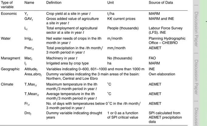
To characterize our model we use regional, national and international sources of data. Table 1 describes the variables included in this study and the source of data. We have included information about crop yield and water requirements of eight representative crops in the 18 regions in the Ebro Basin from 1976 to 2002. Crop yield is defined

10

as the ratio between production (T) and agricultural total area (ha) and data were ob-tained from the Spanish Ministry of Environment (MARM). Economic and geographic variables were mainly obtained from the Spanish Institute of Statistics (INE) while tech-nological variables were taken from FAOSTAT and Food and Agriculture Organization (FAO).

15

To build a proxy variable for irrigation, we used Ebro Basin management authority local data (CHEBRO, 2004) about net water needs of crops. Finally, climatic data such as total precipitation, maximum and mean temperatures, and number of days below 0◦C were taken from the Spanish Meteorological Agency (AEMET) to characterize the impact of climate.

20

2.3 Crop-water production function

We have estimated a crop-water production function that establishes the relationship between crop yield and water applied for a range of crops that represent irrigated agri-culture in the Ebro Basin. The crop-water production function is linear in the deficit irrigation section because all the applied water is used for evapotranspiration, and the

25

(7)

Neverthe-HESSD

7, 5895–5927, 2010

S. Quiroga et al.

Title Page

Tables Figures

◭ ◮

Back Close

Full Screen / Esc

Discussion

P

a

per

|

Dis

cussion

P

a

per

|

Discussion

P

a

per

|

Discussio

n

P

a

per

|

less, non-linear responses indicate that not all water is used by the crop, since some goes to deep drainage and the evapotranspiration production function is really a pro-duction function. The function becomes curvilinear as more of the applied water goes to deep drainage. Generally, a curvilinear function is expressed as a second order polynomial (Al-Jamal, 2000). This function is not unique and varies among crops and

5

zones.

The specified model is:

lnYt=αlnYt−1+β0+β1Lt+β2Mact+β3Mact−n+β4Altitudet+β5Area ebrot

+_β₆_{Irrig area}

t+ +β7Irrigt+β8Irrig2t+β9Preci t+β10T Maxi t+β11T Meani t

+_β₁₂_Fr

i t+β13Drot+εt 10

Where the dependent variable (lnYt) is the natural logarithm of the crop yield for a site

in year t. The explanatory variables were described on Table 1. The subscript i on climate and some water variables refers to the three months periods (i=_{def (Dec, Jan,} Feb), mam (Mar, Apr, May), jja (Jun, Jul, Aug) and son (Sep, Oct, Nov)).

We used OLS to estimate the coeﬃ_{cients. To facilitate the improvement of particular}

15

model estimation for each crop, 95% confidence intervals were estimated assuming normality of the residuals, and significant relations were considered into the estimated model. White’s general test (White, 1980) was used to check conditional heteroscedas-ticity under null hypothesis (Ho) of homoscedasheteroscedas-ticity (Johnston and Dinardo, 2001). Durbin-Watson statistics are used to check autocorrelation existence (Durbin and

Wat-20

son, 1950).

When the parameters α_i are estimated, the marginal eﬀ_{ect of a change in the} ex-planatory variables is given by:

∂E[lnY|Xi]

∂Xi

=_α_i

The signs and magnitude of the marginal eﬀ_{ects indicate the e}ﬀ_{ect of a particular}

in-25

(8)

HESSD

7, 5895–5927, 2010

S. Quiroga et al.

Title Page

Tables Figures

◭ ◮

Back Close

Full Screen / Esc

Discussion

P

a

per

|

Dis

cussion

P

a

per

|

Discussion

P

a

per

|

Discussio

n

P

a

per

|

to be interpreted as semi-elasticities because the model presents a semi-logarithmic transformation. The interpretation is that semi-elasticity is responsible for the percent increase of yields produced by a unit change in the input variable.

In the Ebro Basin there exists a very high variability in precipitation and it is common to observe that recurrent drought periods aﬀ_{ect agricultural production. To date, it is}

5

diﬃ_{cult to characterize droughts because of their spatial and temporal properties and} the range of indicators required (Hayes 2002; Keyantash and Dracup 2002; Bradford 2000). In this work, we use the frequently used Standardized Precipitation Index (SPI, McKee et al., 1993). This index, based on the probability of precipitation for any time scale, calculates the diﬀ_{erence in accumulated precipitation between a selected}

ag-10

gregation period and the average precipitation for that same period, it is an index. The calculation of the SPI for any location is based on the long-term precipitation record for a desired time. This long-term record is fitted to a probability distribution, and is then transformed into a normal distribution, implying values that vary around 0. This allows areas with diﬀ_{erent climates to be relatively compared (McKee et al., 1993; Steinmann}

15

et al., 2005). We have selected 12 months as the aggregated period for calculation. To define the criteria for a drought event we follow McKee et al.’s (1993) table where a drought event occurs when SPI values are−1.0 or less (see Table 2). This criterion was followed in previous detailed works in Spain (Iglesias et al., 2007; Garrote et al., 2007). We, then, construct a dummy variable that equals 1 if the yeart is a drought

20

year (with SPI smaller than−1) and 0 in other cases.

Due to the large number of correlated variables the selection of explanatory vari-ables for model specification is important. Greene (2003) shows two alternatives to follow: (a) an inductive approach, which consists in starting with a reduced model and amplifying it by including more variables to a general model. The main problem

associ-25

(9)

HESSD

7, 5895–5927, 2010

S. Quiroga et al.

Title Page

Tables Figures

◭ ◮

Back Close

Full Screen / Esc

Discussion

P

a

per

|

Dis

cussion

P

a

per

|

Discussion

P

a

per

|

Discussio

n

P

a

per

|

from this over-fitted model are not systematically biased. We therefore, we use the second approach in this paper. Finally, to help in the choice of appropriate models, we have used Akaike (1973) and Schwarz (1978) and adjustedR squared criteria. To complete this process of variable selection, we observe a strong relationship between some of the explanatory variables which might be a source of collinearity problems.

5

Given this possible problem, we calculated the variance inflation factor (VIF) for each of the explanatory variables:

VIF(xk)=

1 1−R2

k

VIF represents the squared standard error (or sampling variance) of ˆβk in the

esti-mated model divided by the squared standard error that would be obtained ifx_k were

10

uncorrelated with the remaining variables (Chatterjee and Hadi, 2006). Thus, we fol-low the folfol-lowing criteria: (i) values larger than 10 give evidence of collinearity and, (ii) a mean of the VIF factor considerably larger than one suggests collinearity. We then proceed to eliminate variables which have a VIF value larger than 10. We proceed in an iterative way when collinearity persists.

15

2.4 Agricultural added value

Agricultural added value variations are characterized as a function of crop yields as follows:

lnGAVt=β0+βilnYi t+ +εt

Where the dependent variable (lnGAV_t) is the natural logarithm of agricultural gross

20

added value for a site in yeartand the subscript i refers to the diﬀ_{erent crops} consid-ered.

(10)

HESSD

7, 5895–5927, 2010

S. Quiroga et al.

Title Page

Tables Figures

◭ ◮

Back Close

Full Screen / Esc

Discussion

P

a

per

|

Dis

cussion

P

a

per

|

Discussion

P

a

per

|

Discussio

n

P

a

per

|

responsible for the percent increase of yields produced by a one percent increase in the input variable.

Diagnostic tests were conducted as in the crop-water production function estimation process.

2.5 Montecarlo risk analysis

5

According to Iglesias and Quiroga (2007), risk analysis bridges the gap between impact evaluation and policy formulation by focusing policy’s interest on consequences (i.e. crop yield) rather than agents (i.e. rainfall or irrigation). There are many definitions of risk but, in a wide sense, risk can be defined as the capacity of a system to suﬀ_er losses when it is exposed to an external stressor.

10

In this paper, we use the Montecarlo method, which is a key component of uncer-tainty and probabilistic risk evaluation, since it allows us to generate random samples of statistical distributions to measure risk (Robert and Casella, 2004; cited in Iglesias and Quiroga, 2007; Hammersley and Handscomb, 1975). In agriculture, Montecarlo simulation oﬀ_{ers a flexible and accurate approach for investigating and understanding}

15

statistical properties of crop yield in response to inputs like irrigation and rainfall (Lobell and Ortiz-Monasterio, 2006). In terms of to water policy, we analyze marginal eﬀ_ects on the statistical model to calculate how a reduction in irrigated area could aﬀ_{ect crop} yield (Iglesias and Quiroga, 2009; Llop, 2008). Using Montecarlo simulations we obtain 10 000 random values of statistical distributions of every crop yield and then analyze

20

the distribution of probabilities to obtain a certain yield (risk level).

2.6 Water policy scenarios

We have evaluated three policy scenarios considering a reduction of agricultural irri-gated land of 10%, 20% and 30%. These scenarios are consistent with a perspective of increased water scarcity and reflect the policy implications of environmental

con-25

(11)

HESSD

7, 5895–5927, 2010

S. Quiroga et al.

Title Page

Tables Figures

◭ ◮

Back Close

Full Screen / Esc

Discussion

P

a

per

|

Dis

cussion

P

a

per

|

Discussion

P

a

per

|

Discussio

n

P

a

per

|

and conserve the ecological health of rivers, thus the Hydrological Plan of the Ebro Basin must accommodate the irrigated land area, review current concessions and se-riously consider the removal of salinised irrigated areas as well as those that consume too many resources due to their low profitability.

On the other hand, the establishment of environmental flows in some sections of the

5

Ebro Basin Rivers means that current irrigation areas will have to be reduced. Cur-rently, there is a provisional minimum flow of between 5% and 10% of current annual average flow which is made by sections. It is important to observe that the minimum ecological flow in the Ebro river mouth has been set at 100 m3s−1. This amount is practically arbitrary, due to the absence of more detailed studies. At this moment,

10

some complementary actions are being taken in order to improve the systems’ basin eﬃ_{ciency. For instance, existing or future infrastructure needs to respect the minimum} ecological flow required downstream (Herranz, 2008; CHEBRO 2004).

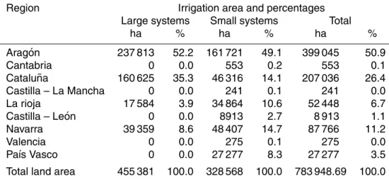
Also, it is well known that irrigated area is a crucial element when talking about agricultural water demand. In Table 3, we can observe a summary of irrigated areas by

15

Community. These are grouped by large and small irrigation systems for each of the nine Autonomous Communities contained within the basin. According to the CHEBRO, the existing concessional irrigated areas’ demand, in the current situation of distribution by crop, is 6310 hm3yr−1 while the current concessional irrigable area is 783 948 ha. Here, Arag ´on and Catalu ˜na account for more than 77% of this area. It is important

20

to say that this demand does not coincide with the annual supplied volume, which depends on the actually irrigated area, and the actual of annual crops among other factors (CHEBRO normative).

Under a hydrologic-hydraulics point of view and according to the regulation and con-cessional guidelines’ adaptations, the maximum possible irrigation area in the future

25

(12)

de-HESSD

7, 5895–5927, 2010

S. Quiroga et al.

Title Page

Tables Figures

◭ ◮

Back Close

Full Screen / Esc

Discussion

P

a

per

|

Dis

cussion

P

a

per

|

Discussion

P

a

per

|

Discussio

n

P

a

per

|

pend on agricultural policy decisions taken by competent institutions. Nevertheless, the COAGRET Report (2007) says that the establishment of future environmental flows on some river sections will imply cuts in current irrigation extensions in order to follow the statements of the Water Framework Directive. It is therefore diﬃ_{cult to think about an} increase in those ha.

5

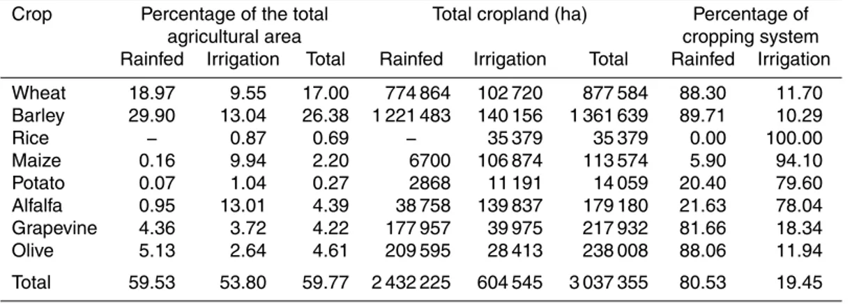
Relative to the total agricultural area in the Ebro Basin, alfalfa, wheat, grapevine, olive, potato, maize and barley are the seven most representative crops in the Ebro Basin since they account for almost 60% of the total agricultural area in this region. Rice does not represent a large percentage of the total cultivated area in the overall basin, but it is the most important crop in the Ebro Delta area and it is an intensively

10

irrigated crop. Alfalfa, maize, potato and rice are mainly irrigated while wheat, barley, grapevine and olive are primarily rainfed crops (Table 4).

3 Results

3.1 Crop-water production functions and agricultural added value

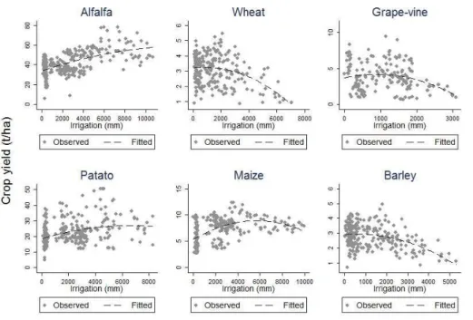
The relationship between crop yields and amount of water for irrigation in the six

rep-15

resentative crops varies with crop and location (Fig. 2). The relationship between crop yield and irrigation is obviously positive in an initial phase but the marginal decrease to scale. For alfalfa, potato and maize, the most irrigated crops considered, the de-creasing phase is not observed within the range of irrigated values considered in this study. For wheat, barley and grapes, optimization of the amount of water is essential.

20

In these crops, additional water beyond a threshold results in reduced output. Rice is not shown since it is always irrigated nor are olives since the amount of irrigated land in this region is relatively small compared to the irrigated land of the other crops.

Irrigated land has evolved diﬀ_{erently for each crop and area considered (Fig. 3). In} the upper basin (Burgos province) the proportion of irrigated area for the cereals crops

25

(13)

HESSD

7, 5895–5927, 2010

S. Quiroga et al.

Title Page

Tables Figures

◭ ◮

Back Close

Full Screen / Esc

Discussion

P

a

per

|

Dis

cussion

P

a

per

|

Discussion

P

a

per

|

Discussio

n

P

a

per

|

scarcity problems in this part of the basin during the period of analysis. In contrast, in the middle basin (Zaragoza province) and the lower basin (Tarragona province) the trend is clearly downward, except in the case of maize in Zaragoza, where the tendency is almost constant. This reflects an increased limitation of irrigation due to prioritization of water for the environment.

5

We estimated crop-water production functions that explain the influence of water on crop productivity and also incorporate a wide range of variables (Table 5). The increas-ing trend in crop productivity is explained largely by technological and management variables. We assume that yield increases due to improved varieties are linked to more intensified management. We tested the adequacy of the functions to represent

10

crop-water production functions as outlined in the methods section; in the cases where regressions present heteroskedasticity the regressions are estimated with the White method (1980) to obtain robust estimates (following Wooldridge, 2003).

As already mentioned, the coeﬃ_{cients of the crop-water production functions can be} interpreted as semi-elasticities. This means that when a unit change is produced in the

15

explanatory variable, the dependent variable experiments proportional changes. In general the eight crop-water production functions present the expected signs ac-cording to the agricultural processes. Irrigation for alfalfa, wheat, rice, potato, maize and barley present a positive impact on the crop yield but this decreases after a given amount of water. Irrigation is not statistically significant for grapevine and olive yield.

20

This may be due to the small area of these crops under irrigation and to the fact that irrigation in these crops is “deficit irrigation” used only to maintain yield during drought periods. Irrigation area also has an important impact on alfalfa, wheat, grapevine, potato, maize and olive. For this last crop, the eﬀ_{ect of irrigation area is the largest.} In contrast, drought does not show significant impacts for all crops. Only wheat,

bar-25

(14)

HESSD

7, 5895–5927, 2010

S. Quiroga et al.

Title Page

Tables Figures

◭ ◮

Back Close

Full Screen / Esc

Discussion

P

a

per

|

Dis

cussion

P

a

per

|

Discussion

P

a

per

|

Discussio

n

P

a

per

|

Table 6 shows the estimated profit function for each crop yield. The estimation of this function has been considered for all crops; however, we only took into account those that are significant. In other words the eﬀ_{ects may be poorly specified for crops} that are not represented in the entire geographic area. We note that when yields of alfalfa, maize, potatoes and wheat increase by 1 unit, the agricultural gross added value

5

increases. A strictly economic analysis might suggest the desirability of a stronger orientation of production towards wheat and maize, because an increase in the yield of these crops has a major impact on the region’s agricultural GAV. However, this does not take into account the cost of virtual water. Even though today the Ebro Delta does not present problems of availability of water the problems associated with the necessity

10

of large amounts of irrigation water that are caused due to factors such as the crop’s characteristics, natural ground permeability and capillary rise of salt water should not be ignored. Therefore, an analysis of water risk management is necessary. In the next section, we analyze the water risk of the selected crops and the impacts of potential changes in water policy.

15

It is important to note that the contribution to the gross added value includes direct payments linked to crop productivity during the period of analysis (before 1986 from the agricultural policy in Spain and since 1986 from the EU Common Agricultural Pol-icy). The recent decupling of productivity and payments, since 2008, may change the relative contribution of each crop to the gross added value.

20

3.2 Montecarlo risk analysis

Statistical properties of crop yield in response to water patterns were derived using Montecarlo simulations in order to asses risk levels. Figure 4 shows the cumulative density probability functions where significant diﬀ_{erences in risk levels between crops} can be observed. According to these cumulative distribution functions, the probability

25

(15)

HESSD

7, 5895–5927, 2010

S. Quiroga et al.

Title Page

Tables Figures

◭ ◮

Back Close

Full Screen / Esc

Discussion

P

a

per

|

Dis

cussion

P

a

per

|

Discussion

P

a

per

|

Discussio

n

P

a

per

|

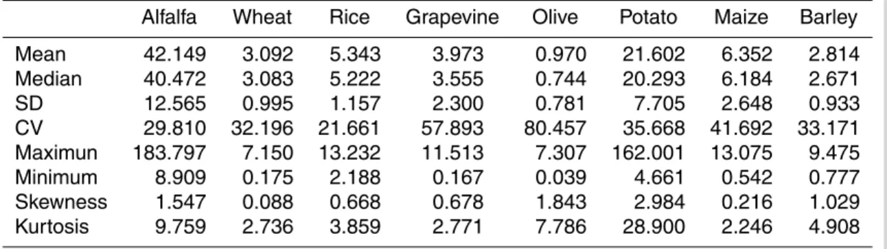
On the other hand, we observed that the skewness coeffi_{cient is above} +_{1 in potato,} olive, alfalfa and barley, indicating that they have an elevated probability of obtaining results above the mean. Also, the skewness coeffi_{cient is greater than 0, indicating} that there is no large probability of having a low yield. The kurtosis coeffi_{cient for every} crop yield is lower than 3, and we have a platykurtic distribution that indicates that the

5

probability distribution functions of the crop yields have a wide peak (a lower probabil-ity than a normally distributed variable of values near the mean) and thin tails (a lower probability than a normally distributed variable of extreme values). Figure 5 presents the distribution function for rice, which is practically normal.

3.3 Water policy scenarios

10

Although irrigation contributes to social welfare in many regions, it cannot be rural de-velopment’s the sole concern. As we mentioned before, nowadays there are no explicit restrictions on the irrigation area in the Ebro Basin. However, within the context of increases of water demands and policy developments such as the Water Framework Directive restrictions context, it is necessary that the Basin Plan consider adaptation

15

measures such as changes in irrigated land to cope with environmental and sustain-ability constraints. Thus, we propose three possible scenarios, in which we assume a reduction of the irrigated area by 10%, 20% and 30%. Table 8 shows the yield changes responding to these scenarios.

A substantial decrease in irrigated land, of up to 30% of total, results in only moderate

20

losses of crop productivity. The response is crop specific, wheat is the least aﬀ_ected and alfalfa is the most aﬀ_{ected. These results contrast with the relative importance of} the crop as measured by the gross added value (Table 6). Both indicators, the gross added value and the changes in crop productivity, are useful to choose adaptation strategies. For example, the contribution of maize to the gross added value is large

25

(16)

HESSD

7, 5895–5927, 2010

S. Quiroga et al.

Title Page

Tables Figures

◭ ◮

Back Close

Full Screen / Esc

Discussion

P

a

per

|

Dis

cussion

P

a

per

|

Discussion

P

a

per

|

Discussio

n

P

a

per

|

resulting economic loss due to limitation in irrigated land is smaller because alfalfa’s contribution to the gross added value is low.

The reductions are consistent given the uncertainty of future policy and our purpose is to show the implications in terms of production risk. Using the models presented in Table 8, we note that these scenarios imply yield losses, ranging from 1% to more than

5

15%. Regardless of the extent of the reduction in irrigated land imposed by the policy, we see that wheat and grapevine do not suﬀ_{er major losses in yield performance,} whereas alfalfa, potato and maize would be aﬀ_{ected considerably given that they are} mostly irrigated crops. Since the irrigation area was not significant for rice (which is 100% irrigated), we cannot observe, using this technique, the amount of decrease in

10

its yield would most likely decline. One important factor to consider is the fact that the losses are not proportional. Therefore, the loss is larger when the irrigation area is reduced from 10–20% scenarios than when it is reduced from 20–30% scenario. Finally, the reductions in crop yields can be used to estimate the necessary incentives for the implementation of environmental goals (Iglesias and Quiroga, 2009).

15

4 Conclusions

Given the pressure, mainly from agriculture, on water in the Mediterranean, this paper presents an analysis of the factors that aff_{ect eight major crops in the Ebro River Basin} including latent risks as well as policies that could be implemented. We analyzed the marginal eff_{ects on the statistical model to calculate the e}ff_{ect of a potential reduction}

20

in irrigated area on crop yield. This study was based on an analysis of demand. Extended water production functions by crop were estimated. These show the ex-pected signs for most of the variables. Focusing on the hydrological variables, our results show that an increase in irrigation and in the irrigated area has a positive im-pact on crop yields. However, the imim-pact of irrigation is not always positive given that

25

(17)

HESSD

7, 5895–5927, 2010

S. Quiroga et al.

Title Page

Tables Figures

◭ ◮

Back Close

Full Screen / Esc

Discussion

P

a

per

|

Dis

cussion

P

a

per

|

Discussion

P

a

per

|

Discussio

n

P

a

per

|

crop yields, except for maize in thesonquarter (Sep, Oct, Nov), which might be due to excessive water from irrigation, given the usual humidity of this time of the year.

A strictly economic analysis might suggest that production could be oriented to wheat and maize, given their impact on agricultural gross value added of the area. However, this does not consider the cost of virtual water. Maize is a major crop in the Ebro

5

Delta, in the low basin, that could suff_{er a reduction on water availability. An analysis of} water risk management is needed. Rice and potatoes show a low variation coeffi_cient, implying low variability. Olive shows low yield and high variability in this area, although under a reduction in irrigated area scenario, this crop is not severely aff_{ected. Potato,} maize and alfalfa are the ones most aff_{ected by a reduction in irrigated area, because}

10

they are mainly irrigated crops.

Finally, the methodology presented here can be extended to examine additional fac-tors that aﬀ_{ect crop yield and interact with water demand, such as climate change,} irrigation systems, and fertilizer application.

Acknowledgement. This research has been supported by the European Commission CIRCE

15

project and the ARCO project of the Spanish Ministry of Environment, Rural, and Marine Aﬀ_airs

(MARM). We also acknowledge the data support of Agencia Estatal de Meteorolog´ı_{a (AEMET).}

References

Acharya, G. and Barbier, E. B.: Valuing groundwater recharge through agricultural production in the Hadejia-Nguru wetlands in northern Nigeria, Agr. Econ., 22, 247–259, 2000.

20

Akaike, H.: A maximum likelihood estimation of Gaussian autoregressive moving average mod-els, Biometrika, 60, 255–265, 1973.

Alcal á, F. and Sancho-Portero, I.: Agua y producci ón agr´ı_{cola: un an álisis econom étrico del}

caso de Murcia, Estud. Agrosoc. Pesqueros, 197, 129–157, 2002.

Al-Jamal, M. S., Sammis, T. W., Ball, S., and Smeal, D.: Computing the crop water production

25

function for onion, Agr. Water Manage., 46, 29–41, 2000.

(18)

HESSD

7, 5895–5927, 2010

S. Quiroga et al.

Title Page

Tables Figures

◭ ◮

Back Close

Full Screen / Esc

Discussion

P

a

per

|

Dis

cussion

P

a

per

|

Discussion

P

a

per

|

Discussio

n

P

a

per

|

Chatterjee, S. and Hadi, A. S.: Regression Analysis by Example. 4th edn. Wiley, New York, USA, 2006.

CHEBRO: Revisi ´on de las Necesidades H´ı_{dricas Netas de los Cultivos en la Cuenca del Ebro,}

1961–2002. Confederaci ´on Hidrogr ´afica del Ebro, Zaragoza, Spain, 2004.

Durbin, J. and Watson, G. S.: Testing for serial correlation in least squares regression, I.,

5

Biometrika, 37, 409–428, 1950.

2000/60/Ce UE Directive: European Commission, 23 October 2000.

Echevarria, C.: A three-factor agricultural production function: the case of Canada, Int. Econ. J., 12(3), 63–75, 1998.

FAOSTAT: Resources (Machinery), Years: 1961–2007, Food and Agriculture Organization of

10

the United Nations (FAO), 2009.

Garrote, L., Flores, F., and Iglesias, A.: Linking drought indicators to policy: The case of the Tagus basin drought plan, Water Resour. Manage., 21(5), 873–882, 2007.

G ómez-Lim ón, J. A. and Riesgo, L.: Irrigation w áter pricing: differential impacts on irrigated

farms, Agr. Econ., 31, 47–66, 2004.

15

Greene, W. H.: Econometric Analysis, 5th ed., Pearson Education, New Jersey, 2003.

Griliches, Z.: Research expenditures, education, and the aggregate agricultural production function, Am. Econ. Rev., 54(6), 961–974, 1964.

Hammersley, J. M. and Handscomb, D. C.: Monte Carlo Methods, Fletcher & Sons Ltd, Norwich, UK, 1975.

20

Hayes, M.: Drought indexes // Drought indices, University of Nebraska, Lincoln, 9 p., 2002. Herranz Lonc ´an, A.: Agua y Desarrollo Econ ´omico en la Cuenca del Ebro (1926–2000), in:

Gesti ´on y Usos del Agua en la Cuenca del Ebro en el siglo XX, edited by: Pinilla Navarro, V., Prensas Universitarias de Zaragoza, 675–703, 2008.

Hussain, S. S. and Mudasser, M.: Prospects for wheat production under changing climate in

25

mountain areas of Pakistan: An econometric analysis, Agr. Syst., 94, 494–501, 2007. Iglesias, A., Garote, L., Flores, F., and Moneo, M.: Challenges to mange the risk of water

scarcity and climate change in the Mediterranean, Water Resour. Manage., 21(5), 227–288, 2007.

Iglesias, A. and Quiroga, S.: Measuring the risk of climate variability to cereal production at five

30

sites in Spain, Clim. Res., 34, 47–57, 2007.

(19)

HESSD

7, 5895–5927, 2010

S. Quiroga et al.

Title Page

Tables Figures

◭ ◮

Back Close

Full Screen / Esc

Discussion

P

a

per

|

Dis

cussion

P

a

per

|

Discussion

P

a

per

|

Discussio

n

P

a

per

|

INE: Statistical Yearbook of Spain and Labour Force Survey (LFS), Years: 1976–2008, National Institute of Statistics, Madrid, Spain, available at: http://www.INE.es, 2009.

COAGRET: Criterios sobre las l´ı_{neas de demandas futuras de agua 2008–2025 en la Cuenca}

Hidrogr ´afica del Ebro Esquema De Temas Importantes: Plan Hidrol ´ogico (2007). Association

of people aﬀ_{ected by big reservoirs report, 2007.}

5

Johnston, J. and Dinardo, J.: M étodos de Econometr´ı_{a, 1a Edici ón, Vicens Vives, Espa ña,}

2001.

Keyantash, J. and Dracup, J. A.: The quantification of drought. An evaluation of drought indices, B. Am. Meteorol. Soc., 83(8), 1167–1180, 2002.

Llop, M.: Economic impact of alternative water policy scenarios in the Spanish production

10

system: an input–output analysis, Ecol. Econ., 68, 288–294, 2008.

Lobell, D. B. and Ortiz-Monasterio, J. I.: Regional importance of crop yield constraints: linking simulation models and geostatistics to interpret spatial patterns, Ecol. Model., 196, 173–182, 2006.

Lobell, D. B., Ortiz-Monasterio, J. I., Asner, G. P., Matson, P. A., Naylor, R. L., and Falcon, W. P.:

15

Analysis of wheat yield and climatic trends in Mexico, Field Crops Res., 94, 250–256, 2005. Lobell, D. B., Ortiz-Monasterio, J. I., and Falcon, W. P.: Yield uncertainty at the field scale

evaluated with multi-year satellite data, Agr. Syst., 92, 76–90, 2007.

MARM: Anuarios de Estad´ı_{stica Agroalimentaria, Years: 1976–2007, Spanish Ministry of}

Envi-ronment and Rural and Marine, Statistical Division, Madrid, 2007.

20

McKee, T. B., Doesken, N. J., and Kleist, J.: The relationship of drought frequency and duration to time scales, 8th Conference on Applied Climatology, Anaheim, CA, UISA Press, 36–66, 1993.

OECD: Sustainable Management of Water Resources in Agriculture, OECD, 2010.

Quiroga, S. and Iglesias, A.: A comparison of the climate risks of cereal, citrus, grapevine and

25

olive production in Spain, Agr. Syst., 101, 91–100, 2009.

Robert, C. P. and Casella, G.: Monte Carlo Statistical Methods (2nd edn.), Springer-Verlag, New York, USA, ISBN 0-387-21239-6, 2004.

Rubinstein, R. Y.: Simulation and the Montecarlo Method, John Wiley & Sons, New York, USA, 1981.

30

Schwarz, G.: Estimating the dimension of a model, Ann. Stat., 6, 461–464, 1978.

Smith, L.: Reforma y descentralizaci ´on de servicios agr´ı_{colas: un marco de pol´}ı_{ticas. Colecci ´on}

(20)

HESSD

7, 5895–5927, 2010

S. Quiroga et al.

Title Page

Tables Figures

◭ ◮

Back Close

Full Screen / Esc

Discussion

P

a

per

|

Dis

cussion

P

a

per

|

Discussion

P

a

per

|

Discussio

n

P

a

per

|

Solow, R. M.: A contribution to the theory of economic growth, Q. J. Econ., 70, 65–94, 1956. Solow, R. M.: The economic of resources or the resources of economics, Am. Econ. Rev.,

64 (May), 1–14, 1974.

Steinmann, A., Hayes, M., and Cavalcanti, L.: Drought indicators and triggers, in: Drought and Water Crises. Science, Technology and Management Issues, edited by: Wilhite, D. A., CRC

5

Press, Boca Raton, FL, 2005.

Stiglitz, J.: Reply, Georgescu-Roegen versus Solow/Stiglitz, Ecol. Econ., 22, 269–70, 1997. Stiglitz, J. E.: A neoclassical analysis of the economics of natural resources, in: Scarcity and

Growth Reconsidered, edited by: Smith, V. K., Johns Hopkins, Baltimore, MD, 1979.

White, H.: A heteroscedasticity-consistent covariance matrix estimator and a direct test for

10

heteroscedasticity, Econometrica, 48, 817–838, 1980.

(21)

HESSD

7, 5895–5927, 2010

S. Quiroga et al.

Title Page

Tables Figures

◭ ◮

Back Close

Full Screen / Esc

Discussion

P

a

per

|

Dis

cussion

P

a

per

|

Discussion

P

a

per

|

Discussio

n

P

a

per

|

Table 1.Description of variables.

Type of Name Definition Unit Source of Data

variable

Economic Yt Crop yield at a site in yeart t/ha MARM

GAVt Gross added value of agriculture K€current prices MARM and INE

a site in yeart

Lt Total employment of agricultural People (thousands) Labour Force Survey

sector at a site in yeart (LFS). INE

Water Irrigi t Net water needs of crops in the ith m/month Planning Hydrographic

month in yeart Oﬃce – CHEBRO

Preci t Total precipitation in theith month/ mm/month AEMET

3 month period in yeart

Managment Mact Machinery in yeart No (thousands) FAO

I_t Irrigated area by crop type ha MARM

Geographic Altitude_t Variables indicating 0–600, 601–1000 and more than 1000 m INE

Area ebrot Dummy variables indicating the 3 main areas of the basin: Own elaboration

Northern, Central and Low Ebro

Climate T Maxi t Maximum temperature in the ith ◦C AEMET

month/3 month period in yeart

T Meani t Average temperature in the ith ◦C AEMET

month/3 month period in yeart

Fri t No. of days with temperatures below 0◦C in theith month/ AEMET

3 month period in yeart

Drot Dummy variable indicating drought 1 or 0 as a function SPI calculated from

years of SPI critical value AEMET precipitation

(22)

HESSD

7, 5895–5927, 2010

S. Quiroga et al.

Title Page

Tables Figures

◭ ◮

Back Close

Full Screen / Esc

Discussion

P

a

per

|

Dis

cussion

P

a

per

|

Discussion

P

a

per

|

Discussio

n

P

a

per

|

Table 2.SPI values and drought intensities.

SPI values

2.0 o more Extremely wet

1.5 to 1.99 Very wet

1.0 to 1.49 Moderately wet

−0.99 to 0.99 Near normal

−1.0 to−1.49 Moderately dry

−1.5 to−1.99 Severely dry

(23)

HESSD

7, 5895–5927, 2010

S. Quiroga et al.

Title Page

Tables Figures

◭ ◮

Back Close

Full Screen / Esc

Discussion

P

a

per

|

Dis

cussion

P

a

per

|

Discussion

P

a

per

|

Discussio

n

P

a

per

|

Table 3.Irrigated area by irrigation systems.

Region Irrigation area and percentages

Large systems Small systems Total

ha % ha % ha %

Arag ´on 237 813 52.2 161 721 49.1 399 045 50.9

Cantabria 0 0.0 553 0.2 553 0.1

Catalu ˜na 160 625 35.3 46 316 14.1 207 036 26.4

Castilla – La Mancha 0 0.0 241 0.1 241 0.0

La rioja 17 584 3.9 34 864 10.6 52 448 6.7

Castilla – Le ´on 0 0.0 8913 2.7 8 913 1.1

Navarra 39 359 8.6 48 407 14.7 87 766 11.2

Valencia 0 0.0 275 0.1 275 0.0

Pa´ı_{s Vasco} ₀ _0.0 _{27 277} _8.3 _{27 277} _3.5

(24)

HESSD

7, 5895–5927, 2010

S. Quiroga et al.

Title Page

Tables Figures

◭ ◮

Back Close

Full Screen / Esc

Discussion

P

a

per

|

Dis

cussion

P

a

per

|

Discussion

P

a

per

|

Discussio

n

P

a

per

|

Table 4.Percentage of agricultural area for selected crops.

Crop Percentage of the total Total cropland (ha) Percentage of

agricultural area cropping system

Rainfed Irrigation Total Rainfed Irrigation Total Rainfed Irrigation

Wheat 18.97 9.55 17.00 774 864 102 720 877 584 88.30 11.70

Barley 29.90 13.04 26.38 1 221 483 140 156 1 361 639 89.71 10.29

Rice − 0.87 0.69 − 35 379 35 379 0.00 100.00

Maize 0.16 9.94 2.20 6700 106 874 113 574 5.90 94.10

Potato 0.07 1.04 0.27 2868 11 191 14 059 20.40 79.60

Alfalfa 0.95 13.01 4.39 38 758 139 837 179 180 21.63 78.04

Grapevine 4.36 3.72 4.22 177 957 39 975 217 932 81.66 18.34

Olive 5.13 2.64 4.61 209 595 28 413 238 008 88.06 11.94

(25)

HESSD

7, 5895–5927, 2010

S. Quiroga et al.

Title Page Abstract Introduction Conclusions References Tables Figures ◭ ◮ ◭ ◮ Back Close

Full Screen / Esc

Printer-friendly Version Interactive Discussion Discussion P a per | Dis cussion P a per | Discussion P a per | Discussio n P a per |

Table 5.Estimated coeﬃ_{cients of crop-water functions, robust t-statistics and}_R2_.

Alfalfa Wheat Rice Grapevine Olive Potato Maize Barley

Ln(Yt−1) 0.4441

[4.73]c

L −0.0116 −0.0118

[3.66]c _[3.66]c

Mac −0.0067 −0.0103 0.0022 0.0013 0.0010 0.0007

[2.05]b _[3.19]c _[4.74]c _[9.62]c _[5.61]c _[3.25]c

Mact−1 0.0069 0.0109 0.0010

[2.16]b _[3.39]c _[3.39]c

Mact−2 0.0005

[1.73]a

Altitude(0−600) −4.80E-05 −6.20E-05

[4.24]c _[4.41]c

Altitude(601−1000) −2.06E-05 2.58E-05 2.66E-05

[4.05]c _[1.69]a _[1.86]a

Altitude(+1000) −1.49E-05 −8.94E-05 −6.57E-05 −1.38E-05 −6.53E-05

[3.36]c _[6.54]c _[4.01]c _[2.16]b _[4.89]c

Cent ebro −0.0412 −0.1006 −0.0781 −0.2954 −0.2646

[1.28] [1.69]a _[1.56] _[6.32]c _[4.15]c

Northern ebro 0.2226 −0.4780 −0.3589 −0.3249 −0.6043

[4.53]c _[2.97]c _[3.08]c _[5.22]c _[4.07]c

Irrig area 0.8531 0.5964 0.9993 1.6479 0.5693 0.7691

[9.65]c _[3.75]c _[4.53]c _[4.22]c _[11.41]c _[9.00]c

Irrig 0.0963 0.2024 0.1543 0.0355 0.0766 0.2496

[7.10]c _[4.73]c _[2.08]b _[2.08]b _[3.35]c _[5.19]c

Irrigˆ2 ₋_0.0083 ₋_0.0447 ₋_0.0213 ₋_0.0002 ₋_0.0027 ₋_0.0649

[5.69]c _[6.59]c _[1.89]a _[0.08] _[1.38]a _[6.24]c

Precdef 0.0015 0.0006

[2.41]b _[3.49]c

Precmam 0.0010

[6.52]c

Precjja 0.0017 0.0006

[2.58]b _[2.88]c

Precson 0.0005 0.0000 0.0004

[3.30]c _[0.20] _[2.33]b

Precyear 0.0001

[1.80]a

T Maxdef 0.0059

[2.17]b

T Maxmam −0.0098 −0.0133

[3.39]c _[4.33]c

T Maxjja −0.0099 −0.0273

[3.10]c _[3.34]c

T Maxson 0.0092 0.0069 0.0187

[2.35]b _[1.88]a _[5.03]c

T Meanyear 0.0474 −0.0879 0.0377 −0.0685 −0.0602 −0.1394

[4.12]c _[3.00]c _[2.24]b _[10.02]c _[2.95]c _[5.40]c

Frdef −0.0022 −0.0019

[1.67]a _[1.41]

Frmam −0.0090 −0.0297 −0.0117

[1.66]a _[2.80]c _[2.53]b

Frson 0.0303 −0.0120 −0.0069

[2.79]c _[4.06]c _[2.11]b

Dro −0.1281 −0.1328 −0.1737

[2.22]b _[1.97]a _[3.75]c

AdjR-squared 0.65 0.63 0.17 0.84 0.41 0.62 0.77 0.55

White test:p-value 0.0008 0.4362 0.3695 0.038 0.6504 0 0.0154 0.5003

(26)

HESSD

7, 5895–5927, 2010

S. Quiroga et al.

Title Page

Tables Figures

◭ ◮

Back Close

Full Screen / Esc

Discussion

P

a

per

|

Dis

cussion

P

a

per

|

Discussion

P

a

per

|

Discussio

n

P

a

per

|

Table 6. Estimated coeﬃ_{cients of profit function (logarithm of the gross added value), robust}

t-statistics (in brackets) andR2.

Coeﬃ_cients

Yield Alfalfa 0.04

[4.58]b

Yield Maize 0.11

[3.56]b

Yield Potato 0.02

[2.49]a

Yield Wheat 0.20

[2.80]b

Constant 9.31

[22.08]b

Observations 133

R-squared 0.31

(27)

HESSD

7, 5895–5927, 2010

S. Quiroga et al.

Title Page

Tables Figures

◭ ◮

Back Close

Full Screen / Esc

Discussion

P

a

per

|

Dis

cussion

P

a

per

|

Discussion

P

a

per

|

Discussio

n

P

a

per

|

Table 7.Statistical properties of yield simulations.

Alfalfa Wheat Rice Grapevine Olive Potato Maize Barley

Mean 42.149 3.092 5.343 3.973 0.970 21.602 6.352 2.814

Median 40.472 3.083 5.222 3.555 0.744 20.293 6.184 2.671

SD 12.565 0.995 1.157 2.300 0.781 7.705 2.648 0.933

CV 29.810 32.196 21.661 57.893 80.457 35.668 41.692 33.171

Maximun 183.797 7.150 13.232 11.513 7.307 162.001 13.075 9.475

Minimum 8.909 0.175 2.188 0.167 0.039 4.661 0.542 0.777

Skewness 1.547 0.088 0.668 0.678 1.843 2.984 0.216 1.029

(28)

HESSD

7, 5895–5927, 2010

S. Quiroga et al.

Title Page

Tables Figures

◭ ◮

Back Close

Full Screen / Esc

Discussion

P

a

per

|

Dis

cussion

P

a

per

|

Discussion

P

a

per

|

Discussio

n

P

a

per

|

Table 8.Yield changes for irrigated area policy scenarios.

Decrease in Changes in crop productivity

irrigated land Alfalfa Wheat Grapevine Olives Potatoes Maize

−10% −4.8 −0.7 −1.5 −2.2 −4.3 −4.8

−20% −11.2 −1.4 −2.9 −4.4 −8.4 −9.4

−30% −15.5 −2.0 −4.3 −6.6 −12.3 −13.7

Yield decrease

0 to -5%

−5% to−10%

(29)

HESSD

7, 5895–5927, 2010

S. Quiroga et al.

Title Page

Tables Figures

◭ ◮

Back Close

Full Screen / Esc

Discussion

P

a

per

|

Dis

cussion

P

a

per

|

Discussion

P

a

per

|

Discussio

n

P

a

per

|

(30)

HESSD

7, 5895–5927, 2010

S. Quiroga et al.

Title Page

Tables Figures

◭ ◮

Back Close

Full Screen / Esc

Discussion

P

a

per

|

Dis

cussion

P

a

per

|

Discussion

P

a

per

|

Discussio

n

P

a

per

|

(31)

HESSD

7, 5895–5927, 2010

S. Quiroga et al.

Title Page

Tables Figures

◭ ◮

Back Close

Full Screen / Esc

Discussion

P

a

per

|

Dis

cussion

P

a

per

|

Discussion

P

a

per

|

Discussio

n

P

a

per

|

(32)

HESSD

7, 5895–5927, 2010

S. Quiroga et al.

Title Page

Tables Figures

◭ ◮

Back Close

Full Screen / Esc

Discussion

P

a

per

|

Dis

cussion

P

a

per

|

Discussion

P

a

per

|

Discussio

n

P

a

per

|

(33)

HESSD

7, 5895–5927, 2010

S. Quiroga et al.

Title Page

Tables Figures

◭ ◮

Back Close

Full Screen / Esc

Discussion

P

a

per

|

Dis

cussion

P

a

per

|

Discussion

P

a

per

|

Discussio

n

P

a

per

|

Fig. 5. Distribution function of simulated rice yield in the low Ebro. Normal distribution with