Two Dimensional Coulomb Potential of Confined Excitons in Quantum Well Structures
M. Solaimani
1,*, M. Izadifard
1,
H. Arabshahi
2,
M.R. Sarkardei
31Faculty of Physics, Shahrood University of technology, Shahrood, Iran 2Physics Department, Payame Noor University, P. O. Box 19395-3697 Tehran, Iran
3 Physics Department, Al-Zahra University, Vanak, Tehran, Iran
(Received 09 October 2012; published online 29 December 2012)
In this study, we have investigated an exciton confined in a single quantum well. For the first time, we have compared the different methods of approximating the effective two dimensional Coulomb potentials which had been previously reported in the literatures. The effect of different previously introduced trial wave functions on the exciton binding energy is also investigated. In order to have a consistent and stable calculation we have tried to find the true region of variations for free parameters of these trial wave func-tions. Effects of the barrier thickness and doping fraction are also investigated.
Keywords: Trial wave functions, Two dimensional Coulomb potentials, Exciton binding energy, Barrier thickness effect, Doping fraction effect.
PACS numbers: 68.65.Fg, 71.35. – y
*[email protected] 1. INTRODUCTION
A better understanding of the electrons and holes behavior in semiconductor materials leads to a deep insight into the physics of the problem. In the nanostructure systems these behaviors become more interesting and this is due to some special characteris-tics like quantum confinement effect. For example, the effect of quantum confinement effect on exciton behav-iors have been also studied vastly during last years [1-2] and thus much experimental [3-4] and theoretical [5-7] works have been devoted to the quantitative under-standing of the physical properties of a single quantum well structure especially in GaAs based ones.
During last decades, different excitonic properties of the nanostructures such as optical properties [8], mag-netic properties [9], and density of states [10], exciton generation rate [11], exciton recombination [12], and transport properties [13] have been extensively studied. The theoretical studies of confined exciton in quantum well structures are usually done with exact diagonali-zation [14], self-consistent approach [15], Quantum Monte Carlo [16], and variational method [17-18]. Among these methods, variational technique is a pretty simple one which its computer implementation is not so difficult.
In this study we have used a variational method with some trial wave functions. Then the binding ener-gy of an exciton confined in a GaAs(1 –x)Alx / GaAs sin-gle quantum well (0 < x < 0.35) is calculated. We have also compared different approximation types of the ef-fective two dimensional Coulomb potential of a confined exciton. Finally we have investigated the effect of dif-ferent existing trial wavefunctions on the exciton bind-ing energy. To find a reliable approach, we have varied their free parameters in different regions of variation and find the exciton binding energy. By comparing our results with previously obtained ones we have tried to find the right free parameters.
2. THEORY
An exciton confined in a single quantum well struc-ture obeys the Hamiltonian of the Senger et al. [19]. In the cylindrical coordinate we have,
2 2
, ,
2
, ,
( )
2 e h e h e h e h
H V z
m z
2 2
2 2
0 1
2 ( e h)
e z z
(1)
where 1 2
0
( )
1 1
e
m m
is the reduced mass
cor-responding to the heavy (+) and light hole (–),
0
1 2 2
z h
m m
, 0
1 2
h m m
are the heavy hole
effec-tive mass along the z direction and in the plane per-pendicular to it [20], ρρe–ρh is the relative coordi-nate and
γ
1 and γ2 are the Kohn-Luttinger band pa-rameters which are the same as those of used in work of Senger et al. These parameters are taken from Ref [21].The variables corresponding to different degrees of freedom are not analytically separable thus direct solu-tion of the equasolu-tion (1) is not simple. Therefore differ-ent approaches have been devised during last decades which include Fourier series expansion [22] and map-ping onto an equation along a distinct direction.
The first way for separation of variables is to take the averaged two dimensional Coulomb potential as [23-24]:
2 2 2
2 2
( ) ( ) ( )
( )
e e h h e h
e h f z f z e
V dz dz
z z
(2)2 1
( ) ( ) 0
2
V
Eb
e h
(3)
2 2
, , , , ,
2
, ,
( ) ( ) 0
2 e h e h e h e h e h e h e h
V z E f z
m z
(4)
Where fe,h(ze,h) are some envelop functions, Eb is the exciton binding energy and Ee,h are the subband ener-gies of the electrons and holes.
Introducing a form factor F(
) as follows is a second way to study the nature of an exciton confined in a quantum well [25]:2 2
/ /
0 1
( ) ( ) iuze ( ) iuzh ( )
e e e h h h
F
duK u dz e f z dz e f z
(5)Where K0 is the modified Bessel function. Now we have two dimensional Coulomb potential as:
2
( ) e ( )
V
F
(6)
Third way for separation of variable is the mapping of the three dimensional Coulomb potential onto an effective two dimensional Coulomb interaction along the ρ direction by introducing of a variational parame-ter η. In this approach the Coulomb potential term in equation (1) can be defined as [26]:
2 2
2 2
0 0
( )
( e h)
e e V z z
(7)
Then in the first order approximation η can be ob-tained from [26]:
2 2
1 1
(ze zh)
(8)By having η the average of two dimensional Cou-lomb potential can be determined. In the fourth way the Coulomb potential can be approximated by [27]:
2 2
2 2
2 2
0 0
( ) ( ) 1
( )
( )
x
e e h h
e h e h
f z f z
e e e
V dz dz
z z
(9)Where 1 x
is a measure of the well width. In order to find the value of
x we have calculated the expecta-tion value of the both sides of the equaexpecta-tion (9):2 2 2
0 2 2
0 2 0 ( ) ( ) ( ) ( ) 1 x
e e h h
e h e h
f z f z e
V dz dz d
z z e e
(10)Then we have changed the value of
x until this equation is satisfied.This effective potential definition technique has been used previously for other excitonic systems like biexcitons in quantum wells [28]. This is because of some advantages, for example using equations (6), (7), or (9) instead of the real three dimensional Coulomb interaction given in equation (1) has the following
bene-fits. Firstly, it separates the Hamiltonian into some one dimensional Schrödinger equation and solution of one dimensional problems is less time consuming. Secondly, it leads to a more stable programming. Thirdly, a quali-tative intuition of the two dimensional Coulomb inter-action behavior related to an exciton confined in a quantum well will be revealed.
There are different methods in order to extract the variational parameters of the trial wave functions or to find the E0 by using equation (16). Differentiation with respect to the variational parameters and equating to zero is a way for this purpose. Plotting the energy as a function of the variational parameters in a multidi-mensional space [29] or using stochastic methods like Monte Carlo [30] and genetic algorithms [31] are other methods which may be used. In this work we have used Monte Carlo schema.
3. VARIATIONAL METHOD
Selecting an appropriate trial wave function with regard to the geometry and typical characteristics of the model system is the main step in the variational scheme. Although there are some attempts to compare different types of trial wave functions for a confined exciton in a quantum well [32-33] but there is not a comprehensive study in this area. In the literatures there are plenty of different types of these functions for a confined exciton in quantum wells. The most fre-quently used trial wave function has been used by Sen-ger et al. [19]:
2 2( )2 2 2
( , )
( ) ( )e e h e
e h
a z z b e e h h
r r
f z f z
(12)
where
, a and b are the free parameters of this trial wave function and fi(zi = e,h) are the envelop functions which reads:, ,
, , ,
, ,
, ,
cos( ), / 2
( )
, / 2
e h e h
e h e h e h e h e h
K z
e h e h
k z z L
f z
A e z L
(13)
where e and h indicate the electron and hole.
, a and b are the free parameters of this trial wave function. An-other form of the trial wave function has the following form [34-35]:2 ( )2
( , ) ( ) ( )e a ze zh
e h e e h h r r f z f z
(14)The other form of the trial wave function reads [36-37]:
0( ) e
(15)which contains no dependence on |ze– zh|. The varia-tional parameter
gives the exciton radius when the system energy is minimized [38].Then the ground state energy can be found by the minimization of:
0 a b, ,
E Min
H
(16)4. RESULTS AND DISCUSSION
The exciton binding energy is written as Eb = Eg + Ee + Eh– Eex where Eg, Ee and Eh are energy gap and subband energies respectively. Eex is defined as the energy eigenvalue of the Hamiltonian in equation (1). The subband energies may found by numerical so-lution of the equations (4) or by using these equations:
1/2 1/2
2
1/2 1/2
2
cos ,
2
cos 2
e e e
e
h h h
h
E m E
L V
E m E
L V
(19)
These equations can be solved by bisection method [42]. Another way to find Eb is to solve equation (3) di-rectly. If a perturbation like an electric field (e.g. along the growth direction) also apply on the system we are not able to use equations (19) for calculating Ee and Eh. In this case we have to perform other numerical meth-ods such as finite difference schema. Here we have used equation (19) in order to find Ee and Eh as a func-tion of the well width.
In order to include the effect of the effective mass mismatch in the well and barrier we have used the Ben-Daniel-Duke boundary condition [43]. The effective mass of the electron and hole in the well has also been obtained by the Vegard law [44].
We have used the material parameters as follows [45]. The total energy band gap difference ∆Eg(x) between GaAs and AlxGa1 –xAs is ∆Eg = 1.155x + 0.37x2(eV). If we show the conduction and valance band offsets as of 0
e
and 0h
respectively then we have 0 e
= AEg ×C and 0h
= AEg × (1 –C) where C a positive value.Now we have used some trial wave functions and tried to find the exciton binding energy by means of the equation (3). We have firstly used the equations (7) and (8) in order to find η and then put it in the equation (3) to find the exciton binding energy. Variations of η and the exciton binding energy as a function of the well width have been shown in the Fig. 1 and 2 respectively. Fig. 1 shows a non-monotonic behavior for the two di-mensional Coulomb interaction η. It reveals that the natures of the two dimensional Coulomb interaction along the
direction (
2 = x2 + y2) is not the same as for three dimensional Coulomb interaction along the r di-rection (r2 = x2 + y2 + z2). We have calculated the exci-ton binding energy by using of the equations (12), (14), (15). The results have been shown in the fig (2). For comparison we have also plotted the exciton binding energy taken from the Ref [20-21]. As the figure shows if we use equation (15) or equation (14) as the trial wave function with a[0,1] &
[0,10 ]8 the consisten-cy between our calculated exciton binding energy and the results of the other groups have shown in the Ref [20-21] is not good. When we apply equation (14) with4 4
[0,10 ] & [0,10 ]
a
or equation (12) with3 , , [0,10 ]
a b
there is better agreement with the Refs [20-21]. In this calculation we have used smaller upper bound for the free parameters a, b,
. If we choose twoor three of these parameters in a larger interval, e.g. 8
, , [0,10 ]
a b
, this always leads to a zero trial wave function. In this case the probability of finding the elec-tron and hole in all the space become zero.Fig. 1 – Variation of the Coulomb separation parameter as a
function of well width
Fig. 2 – Variation of the exciton binding energy as a function of well width for different types of the trial wave functions, different intervals for the free parameters and the results of the Refs [20-21].
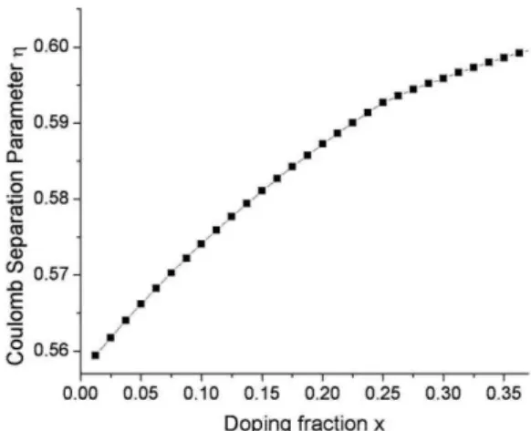
Magnetic field and effective mass dependence of η are also investigated previously [46-47] and here we have evaluated its variation versus the doping fraction x. the result is plotted in the Fig. 3. This plot shows that η has a monotonically increasing behavior. In or-der to calculate the exciton binding energy by equation (9), firstly we have to find the parameter
x. By using equation (10) we found this parameter. The result is presented in the Fig. 4. The same behavior was report-ed by the Ref [48]. The numerical difference is due to the fact that they have applied a dimension less Hamil-tonian but we have used the complete HamilHamil-tonian.Fig. 3 – Variation of the Coulomb separation parameter as a function of the doping fraction x up to 35 %
Fig. 4 – Variation of the trial wave functions free parameter (1 / x) used in the equations 9 as a function of the well width
Fig. 5 – Variation of the exciton binding energy by means of the equations 1, 7, 9, and the results of the Ref [20-21] as a function of the well width
F(
) plays the same role as
in the equation (7). But for comprehensiveness of the work we have presented its analytical form in the equation (6). As it can be seen the equation 7 is closer to the previously obtained re-sults of Ref [20-21]. Although the difference of the three different methods of approximating the effective twodimensional Coulomb potential is not too large but the-se methods of approximating have good advantages in the procedure of making the computational programs more efficient and faster.
In the Fig. 6 and 7 we have investigated the effect of the barrier thickness on the exciton binding energy and the parameter η respectively. In the Fig. 6 the effect of the barrier thickness on the exciton binding energy of a GaAs0.7Al0.3/GaAs quantum well is shown. This figure shows that when the barrier thickness increases the exciton binding energy decreases. Besides, the value of fluctuation (due to numerical inaccuracies) increases with increasing of the barrier thickness. This result is compared with the Ref [20-21). The effect of the barrier thickness on the separation Coulomb parameter η is also investigated. The result which is presented in the Fig. 7 shows that when η decreases the barrier thick-ness increases and has a behavior approximately simi-lar to exciton binding energy.
Fig. 6 – Variation of the exciton binding energy as a function of the well width for different values of the barrier thickness, 30 Å, 500 Å, 1000 Å, infinity, and the results of the Refs [20-21]
Fig. 7 – Variation of the the Coulomb separation parameter
as a function of the well width for different values of the barri-er thickness, 30 Å, 500 Å, 1000 Å, 2000 Å and infinity
5. CONCLUSION
binding energy is investigated. It revealed that the na-tures of the two dimensional Coulomb interaction along the
direction (
2 = x2 + y2) was not the same as for three dimensional Coulomb interaction along the r di-rection (r2 = x2 + y2 + z2). Different shapes of the trial wave function, number of free parameters, and interval of variation of these free parameters in these calcula-tions were comprehensively studied. When we applied equation (14) with a[0,10 ] &4
[0,10 ]4 or equation (12) with a b, ,
[0,10 ]3 there was better agreement with the Refs [20-21]. The effect of the barrier thick-ness on the exciton binding energy and the parameter ηwere investigated. Since we have used the Monte Carlo integration, there were some fluctuations in our results which we tried to reduce them by means of 15 times averaging.
ACKNOWLEDGMENT
We would like to thank Prof. Roman Grill of Charles University in Prague for his kind and helpful e-mail communications. We are also grateful for the financial support of the Iranian nanotechnology initiative council and Shahrood University of Technology.
REFERENCES
1. I.A. Buyanova, M. Izadifard, A. Kasic, H. Arwin, W.M. Chen, H.P. Xin, Y.G. Hong, C.W. Tu, Phys. Rev. B 70, 085209 (2004).
2. I.A. Buyanova, M. Izadifard, W.M. Chen, H.P. Xin, C.W. Tu, Phys. Rev. B69, 201303(R) (2004).
3. S. Adachi, S. Takeyama, Y. Takagi, A. Tackeuchi, S. Muto,
Appl. Phys. Lett.68, 964 (1996).
4. S. Ghosh, T.J.C. Hosea, S.B. Constant, Appl. Phys. Lett.
78, 3250 (2001).
5. M. Solaimani, M. Izadifard, H. Arabshahi, M.R. Sarkardei,
Int. J. Phys. Sci.6, 5364 (2011).
6. F.M. Peeters, J.E. Golub, Phys. Rev. B43, 5159 (1991). 7. K. Chang, F.M. Peeters, Phys. Rev. B63, 153307 (2001). 8. M.E. Flatte, E. Runge, H. Ehrenreich, Appl. Phys. Lett.66,
1313 (1995).
9. D.W. Snoke, W.W. Ruhle, K. Kohler, K. Ploog, Phys. Rev. B 55, 13789 (1997).
10.A. Gladysiewicz, L. Bryja, A. Wojs, M. Potemski, Phys. Rev. B74, 115332 (2006).
11.A.A. Chernyuk, V.I. Sugakov, Phys. Rev. B74, 085303 (2006). 12.E.O. Gobel, H. Jung, J. Kuhl, K. Ploog, Phys. Rev. Lett.51,
1588 (1983).
13.H. Zhao, S. Moehl, H. Kalt, J. Appl. Phys.93, 6265 (2003). 14.R.C. Lotti, L.C. Andreani, Semicond. Sci. Technol. 10,
1561 (1995).
15.I.V. Ponomarev, L.I. Deych, V.A. Shuvayev, A.A. Lisyansk,
Physica E25, 539 (2005).
16.E.G. Wang, Y. Zhou, C.S. Ting, J. Zhang, T. Pang, C. Chen, J. Appl. Phys.78, 7099 (1995).
17.C. Riva, F.M. Peeters, K. Varga, Phys. Rev. B61, 13873 (2000).
18.C. Riva, F.M. Peeters, K. Varga, Phys. Rev. B64, 235301 (2001).
19.R.T. Senger, K.K. Bajaj, X. Wie, S.W. Tozer, Appl. Phys. Lett.83, 2614 (2003)
20.R.L. Greene, K.K. Bajaj, Phys. Rev. B 31, 6498 (1985). 21.A.V. Filinov, C. Riva, F.M. Peeters, Yu.E. Lozovik,
M. Bonitz, Phys. Rev. B 70, 035323 (2004)
22.J.A. Brum, G. Bastard, Phys. Rev. B31, 3893 (1985). 23.A.V. Kavokin, S.I. Kokhanovski, A.I. Nesvizhki,
M.E. Sasin, R.P. Sesyan, V.M. Ustinov, A.Yu. Egorov, A.E. Zhukov, S.V. Gupalov, Semiconductors 31, 950 (1997).
24.C.L.N. Oliveira, J.A.K. Freire, V.N. Freire, G.A. Farias,
Appl. Surf. Sci.234, 38 (2004).
25.N.H. Lu, P.M. Hui, T.M. Hsu, Solid State Commun. 78,
145 (1991).
26.K.S. Lee, Y. Aoyagi, T. Sugano, Phys. Rev. B 46, 10269 (1992).
27.J.J. Liu, S.F. Zhang, Y.X. Li, X.J. Kong, Eur. Phys. J. B
19, 17 (2001).
28.O. Mayrock, H.-J. W¨unsche, F. Henneberger, C. Riva, V.A. Schweigert, F.M. Peeters, Phys. Rev. B 60, 5582 (1999).
29.N. Zettili, Quantum Mechanics: concepts and applications, Second Edition (John Wiley and Sons: 2009).
30.J. Singh, S. Hong, IEEE J. Quant. Electron, 22, 2017 (1986).
31.Y. Hai-Qing, T. Chen, L. Ming, Z. Hao, Commun. Theor. Phys.44, 727 (2005).
32.C.P. Hilton, W.E. Hagston, J.E. Nicholls, Phys. A: Math. Gen.25, 2395 (1992).
33.X.L. Zheng, D. Heiman, B. Lax, Phys. Rev. B 40, 10523 (1989).
34.P. Ballet, P. Disseix, J. Leymarie, A. Vasson, A.-M. Vasson, R. Grey, Phys. Rev. B56, 15202 (1997).
35.R.L. Greene, K.K. Bajaj, Solid State Commun. 45, 831 (1983).
36.S.K. Chang, A.V. Nunnikko, I.W. Wu, L.A. Kolodziejski. R.L. Gunshor, Phys. Rev. B37, 1191 (1988).
37.J.W. Wu, Solid State Commun.67, 911 (1988).
38.A. Bellabchara, P. Lefebvre, P. Christol, H. Mathieu, Phys. Rev. B 50, 11840 (1994).
39.Y. Shinozuka, M. Matsuura, Phys. Rev. B28, 4878 (1983). 40.B. Stebe, L. Stauffer, D. Fristot, Journal de Physique 3,
417 (1993).
41.W. Trzeciakowski, A.P. Roth, Superlattice. Microst.6, 315 (1989).
42.W.H. Press, S.A. Teukolsky, W.T. Vetterling, B.P. Flanner, Numerical Recipes, Third Edition (Cam-bridge University Press: 2007).
43.D.J. Ben Daniel, C.B. Duke, Phys. Rev.152, 683 (1966). 44.S. Jasprit, Semiconductor optoelectronics – physics and
technology (McGraw-Hill Series in Electrical and Compu-ting an Engeeneering: 1995).
45.N.H. Lu, P.M. Hui, T.M. Hsu, Solid State Commun. 78, 145 (1991).
46.X.L. Zheng, D. Heiman, B. Lax, Phys. Rev. B 40, 10523 (1989).
![Fig. 2 – Variation of the exciton binding energy as a function of well width for different types of the trial wave functions, different intervals for the free parameters and the results of the Refs [20-21]](https://thumb-eu.123doks.com/thumbv2/123dok_br/17035988.233356/3.892.477.802.504.749/variation-exciton-function-different-functions-different-intervals-parameters.webp)