www.geosci-model-dev.net/9/2909/2016/ doi:10.5194/gmd-9-2909-2016
© Author(s) 2016. CC Attribution 3.0 License.
DebrisInterMixing-2.3: a finite volume solver for three-dimensional
debris-flow simulations with two calibration parameters – Part 1:
Model description
Albrecht von Boetticher1,3, Jens M. Turowski2, Brian W. McArdell3, Dieter Rickenmann3, and James W. Kirchner1,3 1Department of Environmental Systems Science, ETH Zentrum, CHN H41, 8092 Zürich, Switzerland
2Helmholtz-Centre Potsdam GFZ German Research Center for Geosciences, Telegrafenberg, 14473 Potsdam, Germany 3Swiss Federal Research Institute WSL, Zürcherstrasse 111, 8903 Birmensdorf, Switzerland
Correspondence to:Albrecht von Boetticher ([email protected]) Received: 26 June 2015 – Published in Geosci. Model Dev. Discuss.: 13 August 2015 Revised: 15 July 2016 – Accepted: 18 July 2016 – Published: 31 August 2016
Abstract. Here, we present a three-dimensional fluid dy-namic solver that simulates debris flows as a mixture of two fluids (a Coulomb viscoplastic model of the gravel mixed with a Herschel–Bulkley representation of the fine material suspension) in combination with an additional un-mixed phase representing the air and the free surface. We link all rheological parameters to the material composition, i.e., to water content, clay content, and mineral composi-tion, content of sand and gravel, and the gravel’s friction angle; the user must specify only two free model parame-ters. The volume-of-fluid (VoF) approach is used to com-bine the mixed phase and the air phase into a single cell-averaged Navier–Stokes equation for incompressible flow, based on code adapted from standard solvers of the open-source CFD software OpenFOAM. This effectively single-phase mixture VoF method saves computational costs com-pared to the more sophisticated drag-force-based multiphase models. Thus, complex three-dimensional flow structures can be simulated while accounting for the pressure- and shear-rate-dependent rheology.
1 Introduction
Debris flows typically occur in steep mountain channels. They are characterized by unsteady flows of water together with different contents of clay, silt, sand, gravel, and larger particles, resulting in a dense and often rapidly moving mix-ture mass. They are often triggered by heavy rainfall and
can cause massive damage (Petley et al., 2007; Hilker et al., 2009). Their importance has increased due to extensive set-tlement in mountainous regions and also due to their sensi-tivity to climate change (Guthrie et al., 2010). Their damage potential is not limited to direct impact; severe damage can also be caused by debris flows blocking channels and thus in-ducing overtopping of the banks by subsequent flows (Tang et al., 2011).
Modeling debris flows is a central part of debris-flow re-search, because measuring the detailed processes in debris-flow experiments or in the field is challenging. It is still un-certain how laboratory tests can be scaled to represent real flow events, and the inhomogeneous mixture of gravel and fine material brings about interactions of granular flow and viscous forces such as drag and pore pressure that are dif-ficult to track with the present measurement techniques at reasonable cost. As a consequence, the rheological behavior of debris-flow material remains incompletely understood.
guided by considerations of computational efficiency, here we neglect such phase interactions and restrict ourselves to an effectively single-phase mixture flow simulation. All cur-rently applied debris-flow models that use a two-phase de-scription of the debris-flow material are depth averaged or 2-D. Three-dimensional debris-flow models with momentum exchange between phases have, up to now, been limited to academic cases due to their high numerical costs. Depth-averaged approximations are most applicable to flows over smooth basal surfaces with gradual changes in slope. These approximations are less valid when topography changes are abrupt, such as close to flow obstacles. They are also less applicable when the flow exhibits strong gradients in accel-erations, such as during flow initiation and deposition, or in strongly converging and diverging flows. For such cases, we need a physically complete description of the flow dynamics without depth averaging (Domnik and Pudasaini, 2012). The essential physics of debris flows can be better retained by developing a full-dimensional flow model and then directly solving the model equations without reducing their dimen-sion. The currently available models also contain many pa-rameters that must be estimated based on measurements, or fitted to site-specific field data, limiting their applicability to real-world problems.
Here, we provide a greatly simplified but effective solu-tion linking the rheological model of the debris-flow mate-rial to field values such as grain size distribution and water content. The approach aims to link the knowledge of field experts for estimating the release volume and material com-position with recent advances that account for complex flow phenomena, by using three-dimensional computational fluid dynamics with reasonable computational costs. The parame-ters of the two resulting rheology models for the two mixing fluids are linked to material properties such that the model setup can be based on material samples collected from the field, yielding a model that has two free parameters for cal-ibration. One mixture component represents the suspension of finer particles with water (also simply called slurry in this paper) and a second component accounts for the pressudependent flow behavior of gravel. The two components re-sult in a debris bulk mixture with contributions of the two different rheology models, weighted by the corresponding component concentrations. A third gas component is kept un-mixed to model the free surface. The focus is on the flow and deposition process and the release body needs to be user de-fined.
2 Modeling approach
The debris-flow material can be considered as a combina-tion of a granular component and an interstitial fluid com-posed of a fine material suspension. The interstitial fluid was successfully modeled in the past as a shear-rate-dependent Herschel–Bulkley fluid (Coussot et al., 1998). Because
pres-sure and shear drive the energy dissipation of particle-to-particle contacts, the shear rate substantially influences the energy dissipation within the granular phase. While the two-phase models of Iverson and Denlinger (2001) and Pitman and Le (2005) treated the granular phase as a shear-rate-independent Mohr–Coulomb plastic material, dry gran-ular material has been successfully modeled as a viscoplas-tic fluid by Ancey (2007), Forterre and Pouliquen (2008), Balmforth and Frigaard (2007), and Jop et al. (2006). We follow the suggestions given by Pudasaini (2012) to account for the non-Newtonian behavior of the fluid and the shear-and pressure-dependent Coulomb viscoplastic behavior of the granular phase, as proposed by Domnik et al. (2013). Sev-eral modeling approaches to account for the two-phase nature of debris flows used depth-averaged mass and momentum balance equations for each phase coupled by drag models (e.g., Bozhinskiy and Nazarov, 2000, Pitman and Le, 2005 and Bouchut et al., 2015). Pudasaini (2012) proposed a more comprehensive two-phase mass-flow model that includes general drag, buoyancy, virtual mass, and enhanced non-Newtonian viscous stress in which the solid volume frac-tion evolves dynamically. We apply a numerically more effi-cient method and treat the debris-flow material as one mix-ture (Iverson and Denlinger, 2001, Pudasaini et al., 2005a), with phase-averaged properties described by a single set of Navier–Stokes-type equations. The resulting reduction in nu-merical costs allows us to model the three-dimensional mo-mentum transfer in the fluid as well as the free-surface flow over complex terrain and obstacles.
We assume that the velocity of the gravel is the same as the velocity of the fluid. This assumption is motivated from application and would not be valid for general debris flows with interstitial fluid of low viscosity (i.e., a slurry with low concentration of fine material and large water content). The assumption of equal velocity of gravel and interstitial fluid in one cell leads to a constant composition of the mixture by means of phase concentrations over the entire flow process. This basic model can be seen as a counterpart to the mix-ture model of Iverson and Denlinger (2001), extended by re-solving the three-dimensional flow structure in combination with a pressure- and shear-rate-dependent rheology linked to the material composition. The basic model presented here fo-cuses on the role of pressure- and shear-rate-dependent flow behavior of the gravel, in combination with the shear-rate-dependent rheology of the slurry.
Table 1.Nomenclature.
α phase fraction
αm fraction of the debris mixture (slurry plus gravel)
ρ phase-averaged density,ρi(i=1,2,3)density of phasei,ρexpis a bulk density in experiment
µ phase-averaged dynamic viscosity,µi(i=1,2,3)viscosity of phasei
µ0 maximal dynamic viscosity
µmin minimal dynamic viscosity
µs Coulomb viscoplastic dynamic viscosity
σ free surface tension coefficient
κ free surface curvature
Ddiff diffusion constant
τy yield stress of slurry phase (τy−expis a measured yield stress)
k Herschel–Bulkley consistency index
n Herschel–Bulkley exponent
t time
p,pd pressure, modified pressure
˙
γ shear rate
τ shear stress
τ00 free model parameter (in slurry phase rheology)
τ0 modifiedτ00in case of highC
τ0s yield stress of granular phase modeled with Coulomb friction
C volumetric solid concentration
P0 volumetric clay concentration
P1 reducedP0in case of high clay content
β slope angle
δ internal friction angle
my constant numerical parameter (in gravel phase rheology)
φ volumetric flux (φρdenotes mass flux,φr a surface-normal flux) U velocity
U c interfacial compression velocity g gravitational acceleration
T,Ts deviatoric viscous stress tensor, Cauchy stress tensor (sfor granular phase) D strain rate tensor
I identity matrix
∇ gradient operator
Pudasaini, 2012). Numerical costs are kept reasonable due to the volume-of-fluid (VoF) method (Hirt and Nichols, 1981), which solves only one Navier–Stokes equation system for all phases. The viscosity and density of each grid cell is calcu-lated as a concentration-weighted average of the viscosities and densities of the phases that are present in the cell. Be-tween the two mixing phases of gravel and slurry, the inter-action reduces to this averaging of density and viscosity. In this way, the coupling between driving forces, topography and three-dimensional flow-dependent internal friction can be addressed for each phase separately, accounting for the fundamental differences in flow mechanisms of granular and viscoplastic fluid flow that arise from the presence or absence of Coulomb friction (Fig. 1). We apply linear concentration-weighted averaging of viscosities for estimating the bulk vis-cosity of a mixture for simplicity. Nevertheless, interacting forces such as drag between the grains and the fluid do not appear in our model because we set solid velocity equal to
fluid velocity, and thus, from the physical point of view, this is a debris bulk model.
2.1 Governing equations
Assuming isothermal incompressible phases without mass transfer, we separate the modeled space into a gas region de-noting the air and a region of two mixed liquid components. The VoF method used here determines the volume fractions of all components in an arbitrary control volume by using an indicator function which yields a fraction field for each component. The fraction field represents the probability that a component is present at a certain point in space and time (Hill, 1998). The air fraction may be defined in relation to the fraction of the mixed fluidαmas
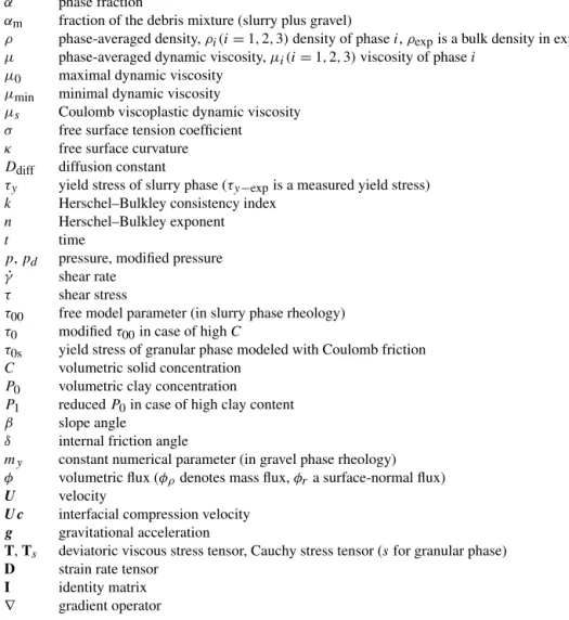
Figure 1.Viscosity distribution (indicated by color scale) along a 28 cm long section through the modeled 0.01 m3release block 0.2 s after release, corresponding to the experimental setup of Hürlimann et al. (2015). The starting motion (black velocity arrows) with corresponding viscosity distribution of the mixture (left) is a consequence of blending pure shear-rate-dependent slurry-phase rheology (center) with the pressure- and shear-rate-dependent gravel phase rheology that accounts for Coulomb friction (right). Because the gravel concentration in this example is low, its effect on the overall viscosity is small.
and the mixed fluid αm may be defined as the sum of the constant fractions of the mixing phasesα2andα3:
αm=α2+α3. (2) The debris bulk motion is defined by the continuity equation together with the transport and momentum equations:
∇ ·U=0, (3)
∂αm
∂t + ∇ ·(Uαm)=0, (4)
and ∂(ρU)
∂t + ∇ ·(ρU×U)= −∇p+ ∇ ·T+ρf, (5) wheretdenotes time andUrepresents the debris bulk veloc-ity field,Tis the deviatoric viscous stress tensor for the mix-ture, ρ is the phase-averaged bulk density,p denotes pres-sure, andf stands for body forces per unit mass. We assume incompressible material and all fractions are convected with the same bulk velocity. Therefore, differences in phase veloc-ities, and thus the interaction forces, such as drag between the grains and the fluid, are neglected. An efficient technique of the VoF method convects the fraction fieldαmas an invari-ant with the divergence-free flow fieldU that is known from previous time steps:
∂αm
∂t + ∇ ·(Uαm)+ ∇ ·(α1Uc)=0, (6) whereUcis an artificial interfacial compression velocity act-ing perpendicular to the interface between the gas region and the mixed liquid phases. The method allows a reconstruction of the free surface with high accuracy if the grid resolution is sufficient (Berberovi´c et al., 2009; Hoang et al., 2012; Desh-pande et al., 2012; Hänsch et al., 2013). The details about the interface compression technique, the related discretization, and numerical schemes to solve Eq. (6) are given in Desh-pande et al. (2012). However, to allow diffusion between the
mixing constituents of the slurryα2and the gravelα3in case of initially unequally distributed concentrations, our modi-fied version of the interMixingFoam solver applies Eq. (6) separately to each mixing component including diffusion:
∂αi
∂t + ∇ ·(Uαi)−Ddiff∇ 2α
i+ ∇ ·(α1Uc)=0, (7) wherei=2,3 denote the slurry and gravel constituents and Ddiffis the diffusion constant that is set to a negligible small value within the scope of this paper.
The discrete form of Eq. (7) is derived by integrating over the volumeV of a finite cell of a grid discretization of the simulated space, which is done in the finite volume method by applying the Gauss theorem over the cell faces. The ad-vective phase fluxesφ1...3 are obtained by interpolating the cell values ofα1,α2, andα3to the cell surfaces and by mul-tiplying them with the fluxφthrough the surface, which is known from the current velocity field. To keep the air phase unmixed, it is necessary to determine the flux φr through the interface between air and the debris flow mixture, and to subtract it from the calculated phase fluxesφ1...3. Inher-ited from the original interMixingFoam solver (OpenFOAM-Foundation, 2016a), limiters are applied during this step to bound the fluxes to keep phase concentrations between 0 and 1. With known fluxesφ1...3, the scalar transport equation for each phase takes the form
∂
∂tαi+ ∇(φi)−Ddiff∇ 2α
i=0. (8)
Equation (8) is the implemented scalar transport equation solved for each constituent using first-order Euler schemes for the time derivative terms, as has been recommended for liquid column breakout simulations (Hänsch et al., 2013).
After solving the scalar transport equations, the complete mass fluxφρis constructed from the updated volumetric frac-tion concentrafrac-tions:
Figure 2.Longitudinal section through a debris-flow front discretized with finite-volume cells, showing the constitutive equations for one cell with densityρand viscosityµ, given the densitiesρ1...3, viscositiesµ1...3, and proportionsα1...3of phases present. The numbers 1, 2,
and 3 denote the air (white colored cell content), mud, and gravel phases, respectively.
whereρ1...3denote the constant densities of the correspond-ing phases andφ1...3are the corresponding fluxes. The com-plete mass fluxφρ is used in the implementation to describe the second term of the momentum equation (Eq. 14) as de-scribed in Appendix A. Figure 2 illustrates how the phase volume distributionsα1(air),α2(slurry), andα3(gravel) are used to derive cell-averaged properties of the continuum.
The conservation of mass and momentum is averaged with respect to the phase fraction α of each phase. The density field is defined as
ρ=X i
ρiαi, (10)
whereρi denotes density of phaseiand the phase density is assumed to be constant.
The deviatoric viscous stress tensor T is defined based on the mean strain rate tensorDthat denotes the symmetric part of the velocity gradient tensor derived from the phase-averaged flow field:
D=1
2[∇U+(∇U) T
], (11)
and
T=2µD. (12)
Equation (12) was derived accounting for Eq. (3) andµ is the phase-averaged dynamic viscosity, which is simplified in analogy to Eq. (10) as the concentration-weighted average of the corresponding phase viscosities:
µ=X i
µiαi. (13)
With the continuity Eq. (3), the term∇ ·Tin Eq. (5) is written as∇ ·(µ∇U)+(∇U)· ∇µto ease discretization. The body forcesf in the momentum equation account for gravity and for the effects of surface tension. The surface tension at the interface between the debris-flow mixture and air is modeled as a force per unit volume by applying a surface tension coef-ficientσ. Although the surface tension can be considered to have a minor influence on debris-flow behavior, it allows an adequate reproduction of surface-flow patterns observed in laboratory-scale experiments used for validation (von Boet-ticher et al., 2015). The momentum conservation including gravitational accelerationgand surface tension is defined in our model as
∂(ρU)
∂t + ∇ ·(ρU×U)= −∇pd+ ∇ ·(µ∇U)
+(∇U)· ∇µ−g·x∇ρ+σ κ∇α1, (14) whereκdenotes the local interfacial curvature andx stands for position. The modified pressurepd is employed in the solver to overcome some difficulties with boundary condi-tions in flow simulacondi-tions with density gradients. In case the free surface lies within an inclined wall forming a no-slip boundary condition, the normal component of the pressure gradient must be different for the gas phase and the mixture due to the hydrostatic componentρg. It is common to intro-duce a modified pressurepdrelated to the pressurepby
gradient as well as a body force due to gravity (Berberovi´c et al., 2009).
Together with the continuity Eq. (3), Eq. (14) allows us to calculate the pressure- and gravity-driven velocities. The corresponding discretization and solution procedure with the PISO (pressure-implicit with splitting of operators; Issa, 1986) algorithm is provided in Appendix A. The set of equa-tions governing the flow in our model are Eqs. (8)–(15) to-gether with the continuity Eq. (3). In the following section, we present the rheology models that define the viscosity components for Eq. (13).
2.2 Rheology model for the fine sediment suspension The viscosity of the gas phase,µ1is chosen constant. The in-troduction of two mixing phases is necessary to distinguish between the pressure-dependent flow behavior of gravel and the shear-thinning viscosity of the suspension of finer parti-cles with water. The rheology of mixtures of water with clay and sand can be described by the Herschel–Bulkley rheology law (Coussot et al., 1998), which defines the shear stress in the fluid as
τ =τy+kγ˙n, (16) where τy is a yield stress below which the fluid acts like a solid, k is a consistency index for the viscosity of the sheared material,γ˙ is the shear rate, andndefines the shear-thinning (n <1) or shear-thickening (n >1) behavior. In OpenFOAM, the shear rate is derived in 3-D from the strain rate tensorD:
˙
γ =√2D:D. (17) The shear rate is based on the strain rate tensor to exclude the rotation velocity tensor that does not contribute to the deformation of the fluid body. The model can be rewritten as a generalized Newtonian fluid model to define the shear-rate-dependent effective kinematic viscosity of the slurry phase as
µ2=k| ˙γ|n−1+τy| ˙γ|−1 (18) if the viscosity is below an upper limitµ0and
µ2=µ0 (19) if the viscosity is higher, to ensure numerical stability.
With n=1, the model simplifies to the Bingham rheol-ogy model that has been widely used to describe debris-flow behavior in the past (Ancey, 2007). It may be reasonable to imagine the rheology parameters to be dependent on the state of the flow. However, even with the implicit assumption that the coefficients are a property of the material and not of the
state of the flow, the Herschel–Bulkley rheology law has been rarely applied in debris-flow modeling due to three rheology parameters. We avoid this problem by assuming some rheol-ogy parameters to be defined by measurable material proper-ties as described below.
Determination of rheology model parameters based on material properties
Results from recent publications allow the reduction of the number of free Herschel–Bulkley parameters to two. If the coarser grain fraction is assumed to be in the gravel phase, the Herschel–Bulkley parameters for the finer material can be linked to material properties that can be measured us-ing simple standard geotechnical tests. Accordus-ing to Cous-sot et al. (1998), the exponentncan be assumed constant at 1/3, andkcan be roughly estimated asbτy, with the constant b=0.3 s−nfor mixtures with maximum grainsizes<0.4 mm (Coussot et al., 1998). An approach for estimating the yield stressτy based on water content, clay fraction and compo-sition, and the solid concentration of the entire debris-flow material was proposed by Yu et al. (2013) as
τy=τ0C2e22(CP1), (20) whereC(a constant) is the volumetric solid concentration of the mixture (the volume of all solid particles including fine material relative to the volume of the debris-flow material including water),P1=0.7P0whenP0>0.27, andP1=P0 ifP0<=0.27, and
P0=Ckaolinite+chlorite+1.3Cillite
+1.7Cmontmorillonite, (21)
where the subscript ofCrefers to the volumetric concentra-tion (relative to the total volume of all solid particles and water) of the corresponding mineral. The discontinuity ofP1 at a modified clay concentration ofP0=0.27 is a coarse ad-justment to a more-or-less sudden change observed in the ex-perimental behavior.
ForC <0.47,τ0is equal toτ00 and otherwiseτ0can be calculated by
τ0=τ00e5(C−0.47), (22) whereτ00 is the remaining free parameter which we use to account for the grid-size dependency of the shear rate (Yu et al., 2013). The change in the definition ofτ0at solid con-centrations exceeding 0.47 accounts for a threshold between weak coherent and medium coherent debris-flow material.
from a reservoir into an inclined channel of 0.2 m width and by increasing the inclination slightly until remobilization oc-curred after the material came to rest. The experimental yield stressτy−expwas then simplified as
τy−exp=ρexpghsin(β), (23) whereρexpis the density of the applied mixture,his the max-imum accumulation thickness of the deposit, and β is the slope inclination. In addition, they compared the calculated yield stress of Eq. (20) with experimental yield stresses re-ported by a number of authors including Coussot et al. (1998) and Ancey and Jorrot (2001). Ancey and Jorrot (2001) used 2 and 3 mm glass beads in a kaolinite dispersion as well as fine sand–kaolinite–water mixtures. Up to yield stresses of about 200 Pa the yield stresses estimated by Eq. (20) fit the observed ones well. Thus, the yield stresses of sand–clay mixtures with water can be estimated using Eq. (20) based on the volumetric concentration of the debris in the water–solids mixture and based on the percentages of different clays in the fraction of fine material. Adjustments to the numbers for cal-culating P0may be necessary to account for the activity of other clays.
The remaining uncertainties concern the assumptions about the value ofn, and thatkcan be defined in such sim-ple dependency toτyin the presence of coarser sand. Experi-ments seem to confirm thatnincreases in presence of coarser material (Imran et al., 2001), but further research is needed to quantify this effect. Remaitre et al. (2005) foundnto vary from 0.27 to 0.36. Schatzmann et al. (2003) used n=0.33 to reproduce measured curves obtained with a mixture of 27.5 volumetric percent slurry with 30 % gravel where gravel grain sizes ranged from 3 to 10 mm. He appliedn=0.5 to fit the Herschel–Bulkley model to the experiment with 22.5 % slurry and 30 % gravel. Based on the laboratory-scale exper-iments that are presented in von Boetticher et al. (2015), we have chosen n=0.34 to obtain the best fit for the simula-tion of large-scale debris-flow experiments. However, other debris-flow mixtures may demand a recalibration of n be-cause natural debris-flow mixtures cover a wide spectrum from shear thinning to shear thickening behavior. Thus, we consider nas the second model calibration parameter. The model calibration is constricted to τ00, which accounts for the grid resolution sensitivity of the shear rate andn, which allows adjusting the model to shear thinning or shear thick-ening mixtures.
2.3 Representation of gravel by a Coulomb viscoplastic rheology
With a novel model, Domnik and Pudasaini (2012) showed that introducing a Coulomb viscoplastic sliding law to replace a simple no-slip boundary condition completely changes the flow dynamics and the depth variations in veloc-ity and dynamic pressure. They show that with a Coulomb
viscoplastic sliding law, the observable shearing mainly oc-curs close to the sliding surface, in agreement with observa-tions but in contrast to the no-slip boundary condition. In our model, during acceleration and high-speed flow, the shear-thinning behavior of both the fluid and the granular phase dominate the viscosity. However, the representation of gravel by a pressure and rate-dependent Coulomb viscoplastic rhe-ology becomes important as soon as the material experiences high pressures, accompanied by reduction in shear due to de-celerations. This may be caused by channel slope reductions, diverging or converging flows, and interactions with obsta-cles (see, e.g., Pudasaini et al., 2005b; Domnik et al., 2013). Flows of granular material could be modeled as viscoplastic fluids (Ancey, 2007; Forterre and Pouliquen, 2008; Balm-forth and Frigaard, 2007; Jop et al., 2006) as cited by Dom-nik and Pudasaini (2012). Based on Ishii (1975), the granular Cauchy stress tensorTs can be written as
Ts= −pI+2µsD, (24)
wherepIis the pressure times the identity matrix andµs is the corresponding dynamic viscosity, which was modeled by Domnik and Pudasaini (2012) as
µs=µmin+ τ0s ||D||[1−e
−my||D||], (25)
whereµmin is a minimal dynamic viscosity, τ0s is a yield stress, and||D||is the norm of the strain-rate tensor defined by the authors as
||D|| =p2t r(D2). (26)
In Eq. (25),my is a numerical parameter with units of sec-onds which we will keep constant. Domnik et al. (2013) de-rived the yield stress as a pressure-dependent Coulomb fric-tion,p·sin(δ)whereδis the internal friction angle:
µ3=µmin+p·sin(δ) ||D|| [1−e
−my||D||]. (27)
Here, this Coulomb viscoplastic rheology model is used to describe the gravel phase. The pressure- and shear-dependent viscosity is calculated in every cell with the corresponding local pressurep and strain-rate tensor D derived from the phase-averaged flow field.
Gravel phase properties
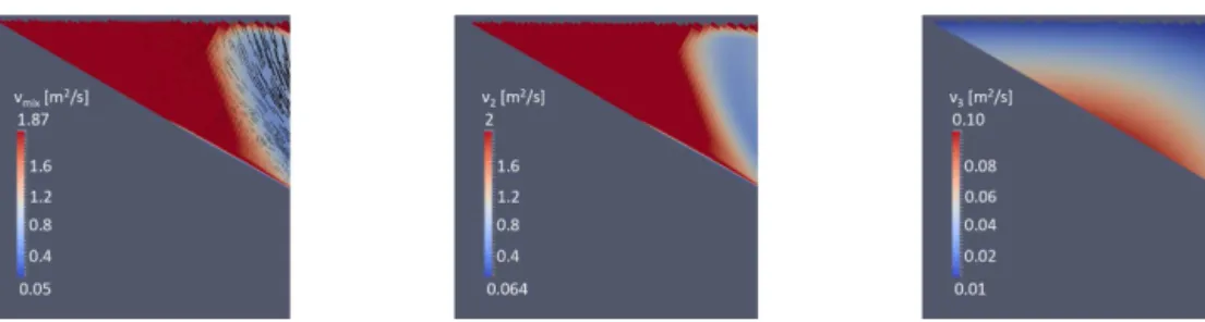
Figure 3.Dependency of the kinematic gravel phase viscosityνs (normalized by density) on the norm of the strain rate tensor||D||
at different levels of pressure normalized by density formy=1 s,
my=0.2 s, and a friction angleδ=36◦.
regions. For smaller values ofmy, the transition is smoother. In the absence of shear, to achieve a viscosity representing a Coulomb friction equal top·sin(δ)wherep is the local pressure,myneeds to be equal to 1 s. However, the develop-ment ofµs under large pressure or strong shear is the same for both my=1 s andmy=0.2 s. So, we choosemy to be constant and equal to 0.2 s for all simulations. However, we mention that parts of the nearly immobile material that ex-perience little pressure (in general, immobile material close to the surface) show a significant reduction in viscosity when my=0.2 s (Fig. 3). As a consequence,myminimally affects debris-flow release and flow at large scales, but slowly mov-ing material with a shallow flow depth in a run-out plane may develop front fingering (which is dependent on and sensitive to the value ofmy) by allowing sudden local solidification.
For small friction angles, the modeled viscosity of the gravel phase decreases rapidly with increasing shear. Larger friction angles increase the viscosity and extend the pressure dependency to larger shear rates (Fig. 4). We estimated the friction angle δ based on the maximum angle of repose in tilt-table tests of the gravel. In our laboratory experiments, we determined the friction angle in a simple adaptation of the method of Deganutti et al. (2011) by tilting a large box with loose material until a second failure of the material body occurred.
In analogy to the Herschel–Bulkley implementation, an upper limit for the viscosity is implemented to maintain nu-merical stability. Pressure-dependent viscosity in the incom-pressible Navier–Stokes equations causes numerical instabil-ity as soon as the eigenvalues of the symmetric part of the lo-cal velocity gradient become larger than 1/(2(δµ/δp)). Fol-lowing Renardy (1986), we locally limit the viscosity to keep it below a corresponding local stability limit.
Figure 4.Dependency of the kinematic gravel phase viscosity (for friction angleδ=25◦and 40◦) on the norm of the strain rate tensor
||D||at different levels of pressure normalized by density, formy= 1 s.
3 Quality characteristics of the model
3.1 Modeled interaction between granular and fluid constituents
As stated before, debris flows are multiphase flow processes where solid particles and interstitial fluid and probably gas phases interact. The model presented applies cell-averaged values of the mixtures and does not allow for consideration of interactions between a granular and a fluid phase. However, a dynamic evolution of the gravel and slurry concentration is the necessary next step. A two-way coupling to a Lagrangian particle simulation could deliver an alternative solution. 3.2 Advantages of full-dimensional mass flow
tran-sitions from rapid flow to the deposition regime, shock-like structures form and a predominantly basal sliding flow changes into a surface boundary layer flow, which, further downstream, quickly slows and eventually settles. This tran-sition has been observed in the laboratory with granular PIV (particle image velocimetry) measurements for rapidly moving granular material impinging on a rigid wall perpen-dicular to the bed, leading to strong shearing through the flow depth (Pudasaini et al., 2007). The scaling of impact pressures on rigid obstacles with obstacle size is complex (Bugnion et al., 2012); the spatial distribution depends on the local flow structure (Scheidl et al., 2013) and the distri-bution of forces over the flow depth is non-trivial and highly dynamic (Berger et al., 2011). Thus, although the rapid flow regime can be reasonably approximated by a depth-integrated dynamical model, adequately simulating the de-position regime and interactions with obstacles requires re-solving the three-dimensional flow structure. Our attempts to consider the three-dimensional flow structure of debris flows were motivated by the need to predict the dynamic loading of shallow landslide impacts to flexible protection barriers (von Boetticher, 2013) and the corresponding re-search in full-dimensional model development is a topic of ongoing interest (Leonardi et al., 2016). In the model pre-sented here, we aim to account for both the three-dimensional flow structure and the corresponding influence of pressure. Domnik et al. (2013) developed a two-dimensional Coulomb viscoplastic model and applied it for inclined channel flows of granular materials from initiation to deposition. They pro-posed a pressure-dependent yield strength to account for the frictional nature of granular materials. The interaction of the flow with the solid boundary was modeled by a pressure- and rate-dependent Coulomb viscoplastic sliding law. In regions where depth-averaging becomes inaccurate, like in the initia-tion and deposiinitia-tion regions, and particularly in interacinitia-tions with obstacles, three-dimensional models are essential be-cause in these regions the momentum transfer must be con-sidered in all directions. Thus, prediction of the velocity vari-ations with depth, and the full dynamical and internal pres-sure, can only be obtained through three-dimensional mod-eling (Domnik et al., 2013). These dynamical quantities can be adequately described by a Coulomb viscoplastic mate-rial with a pressure-dependent yield stress expressed in terms of the internal friction angle, the only material parameter in their model. The pressure dependency introduces an addi-tional need to account for the three-dimensional flow struc-ture.
3.3 Effects of time step size on rheology
Brodani-Minussi and deFreitas Maciel (2012) simulated dam-break experiments of a Herschel–Bulkley fluid using the VoF approach, and compared the results with pub-lished shallow-water-equation-based models. Especially for the first instant after the material release, the application
of shallow-water equations seems to introduce errors that are propagated throughout the process, leading to erroneous run-out estimates. A similar problem arises when modeling debris-flow impacts against obstacles. Simulating the impact of material with velocity-dependent rheology that is kept constant over the time step although it actually changes with the changing flow leads to an accumulating over- or under-estimation of energy dissipation. For example, if a shear-thinning material undergoes acceleration, and thus an in-crease in its shear rate, viscosity calculations based on its shear rate at the beginning of each time step would overes-timate the average viscosity (and underesoveres-timate the change in shear rate) over the whole time step. As a consequence, the resulting viscosity at the end of the time step would be underestimated, which would amplify the overestimation of viscosity in the next time step. Conversely, at an impact, the sudden deceleration causes an underestimation of viscosity over the time step length, leading to an overestimated veloc-ity that again amplifies the underestimation of the viscosveloc-ity in the next time step. As a result, flow velocities change with changing time step size. Avalanche codes such as RAMMS (Christen et al., 2007) deal with this problem by calibrating the model to data from previous events at the same location and similar conditions. But changes in release volume or po-sition can lead to different accelerations and corresponding changes in the automatic time step control can alter the de-velopment of rheology over time. As long as a flow stage is reached where the flow stops accelerating, the influence on the final front velocity should be negligible. However, debris-flow models which do not iteratively adjust viscosity can-not accurately simulate impacts. Here, our model constitutes a significant improvement, since in the three-dimensional solver we presented, the viscosity bias was reduced by im-plementing a corrector step: taking the average between the viscosity at the beginning of the time step and the viscosity that corresponds to the velocity field at the end of the time step, the time step is solved again, leading to a better calcu-lation of the velocity. This step can be repeated, according to user specifications, to correct the viscosity several times. Al-though this procedure increases numerical calculation time, it clearly reduces the time-step dependency of the simula-tion. Some dependency on the time step is still present when modeling the collapse of material columns, but the origin of this problem is different because it occurs also for Newtonian fluids.
3.4 Effect of grid resolution on rheology
Figure 5.Iso-view sketch of the hillslope debris-flow flume. Mate-rial (b) is released from the reservoir at the top by the sudden verti-cal removal of a gate (a) and flows down a steep slope (c) followed by a gently inclined run-out plane (d).
short channel (Scheidl et al., 2013), a cell height of 1.5 mm, which is of the order of the laboratory rheometer gap, was still not fine enough to reach the limit of grid sensitivity. The free model parameterτ00influences the shear-rate-dependent term of the viscoplastic rheology model and can be used to adjust the simulation to the grid resolution. As long as the gravel phase and grid resolution do not change, it should be possible to model different water and clay contents based on one calibration test. However, as the composition changes, bothτyandτ00must change commensurately, since a change in yield stress affects the shear rate. Our procedure for ad-justing to different mixtures based on one calibrated test is to perform one iteration step for the yield stress of the new mix-ture. By calculatingτy based on the originalτ00value from the calibration test but with the new material composition, an updated yield stress of the new mixture is determined. Rais-ing or lowerRais-ingτ00by the same ratio as the change from the original yield stress of the calibration test to the updated yield stress generates the finalτyas it is applied to the simulation of the new mixture.
The viscosity of the granular phase is averaged over the cell faces to avoid discontinuous viscosity jumps between cells, which may cause instability due to the sensitivity of in-compressible solvers to pressure-dependent viscosity. How-ever, thin cells that allow a precise calculation of the shear gradient lead to a preferred direction of the smoothing of the granular phase’s viscosity which may introduce physically unrealistic behavior. Cell length (in the flow direction), cell width, and cell height should at least be of the same order. Especially when front fingering is of interest, a grid resolu-tion test should be carried out, ensuring that front instability is not caused by a large aspect ratio of the cell dimensions.
Figure 6.Laser measurement and corresponding simulated values of the flow head over time, 1 m downslope of the gate for hillslope debris-flow flume experiments with water content of 28.5 %. The laser data were box averaged over 10 ms.
4 Illustrative simulations
Because the purpose of this paper is to illustrate the solver structure and model basis, we defer a detailed discussion of model performance to our next paper, in which the model is validated against laboratory tests, large-scale experiments, and natural hillslope debris-flow events. Here, we discuss only the efficiency of the solver itself, together with tests of the model accuracy in a gravity-driven open channel flow. 4.1 Test case of a dam-break-released debris-flow
mixture stopping on an inclined plane
Figure 7.Simulated deposit (view from top in a hillslope debris-flow flume experiment) for a mixture with 28.5 % water content and
δ=36◦. The thick solid lines indicate the experimental deposit and vertical thin lines represent the 20 cm spacing marks in the experi-mental slope.
and simulated flow depths at such small scales are only ap-proximate due to the surface disturbance by coarser grains that cause significant fluctuations in surface elevation. How-ever, the arrival time, the maximal flow depth, and the decay of surface elevation over time were considered to be suitable for comparison to the model. The model performance was evaluated by comparing the deposition patterns, travel times, and time series of flow depths in the simulations and experi-ments. The simulated flow depths reproduced the laser signal with respect to both time and amplitude (Fig. 6) and the pre-dicted run-out deposit was in almost perfect agreement with the shape of the experimental deposit (Fig. 7). The simulation setup of the test case is included in the Supplement.
4.2 Comparison to a drag-force-based Eulerian multiphase model
In comparison to drag-force-based Eulerian multiphase mod-els, the volume-of-fluid approach applied here significantly reduces calculation time. For an estimate, we compared our model with the OpenFOAM standard solver mul-tiphaseEulerFoam. We selected the official tutorial case damBreak4phaseFine but turned the water phase into mer-cury to gain a three-phase test case, and applied the stan-dard solver settings from the case to our model. On a Cen-tOS 6.3 Linux machine with 31 GiB memory and 16 Intel Xeon CPU E5-2665 @ 2.40 GHz processors, our model re-sulted in a 5.5 times faster calculation with a comparable col-lapse of material columns (Fig. 8). For the sake of complete-ness, our calculation included one iterative viscosity correc-tion step, thus the model efficiency can be estimated to be about 10 times higher than a drag-force-based phase coupling approach.
Figure 8.Phase positions in a dam break standard test-case tion using a drag-based three-phase multiphaseEulerFoam simula-tion (air is transparent) as background shapes with the correspond-ing phase positions of our model as wire frame in front (with white mercury and black oil). The visualized time steps correspond to 0, 0.1, 0.2, 0.3, 0.4, and 0.5 s.
5 Conclusions
The new debris-flow solver has two main strengths. First, it can model three-dimensional flows and their impact against complexly shaped objects, representing the processes at a high level of detail and reasonable computational costs. Sec-ond, its design allows simulating different debris-flow mate-rial compositions with a reduced calibration process as long as the simulation grid does not change, because the calibra-tion parametersτ00andnare largely insensitive to changes in water content, channel roughness, or release volume. Due to the pressure- and shear-dependent rheology used here, realis-tic deposit geometries and release dynamics can be achieved, as presented and discussed on the basis of test cases in the next paper. By systematically excluding unknown parameters from the model architecture and by accounting for known flow phenomena in a simplified way, we have developed a debris-flow model whose parameters can be roughly esti-mated from material composition, leaving only two calibra-tion parameters. The concept is promising; however, impor-tant parts of phase interactions are neglected in favor of lower numerical costs.
6 Code availability
Appendix A
The following section describes the detailed implementation of the PISO iteration procedure as described in Deshpande et al. (2012). By applying the continuum surface force model of Brackbill et al. (1992), the volume integral of Eq. (14) is given as
Z
i ∂ρU
∂t dV+
Z
∂i
(ρU U)·ndS
= −
Z
i
∇pddV−
Z
i
g·x∇ρdV +
Z
i
σ κ∇α1dV
+
Z
∂i
(µ∇U)·ndS+
Z
i
∇U· ∇µdV . (A1)
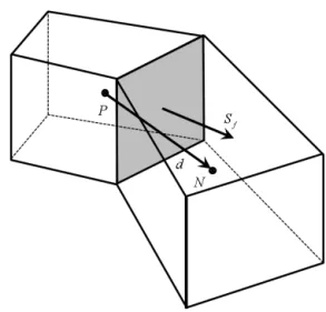
The computational domain is discretized into finite-volume cells. Each cell is considered as the owner of exactly one face that it shares with an adjacent neighbor cell, thus each face has a defined owner cell. A surface normal vec-torSf with magnitude equal to the surface area of the face is defined on the face pointing outward from the owner cell (Fig. A1). The value at facef of any variableχ calculated in the cell centers asχP andχN (Fig. A1) can be derived by interpolation using a mixture of central and upwind schemes:
χf =γ (χP−χN)+χN, (A2)
with a weighting factorγ that can account for the flow di-rection based on the chosen interpolation scheme and flux limiter. In case of a linear interpolation scheme and a flux limiterψ,γ can be defined as
γ =ψf N
d +(1−ψ ) φf |φf|
, (A3)
where d is the distance between the cell centersP andN andf Nis the distance from the face center to the cell center N. The face flux denoted as φf serves as a switch to ac-count for the flow direction since it turns negative when the flow is fromN toP (Berberovi´c et al., 2009). Several lim-iters are implemented (OpenFOAM-Foundation, 2016b); we chose the van Leer scheme and assumed uniform grid spac-ing to simplify the followspac-ing explanations withf N/d=0.5. Variables that are evaluated at the cell faces are sub-scripted by f. Due to stability problems that arise from the pressure–velocity coupling in collocated meshes (Ferziger and Peric, 2002), the pressure is solved for the cell centers, whereas the velocity is interpolated to the cell faces within the PISO loop.
With the switch function
ζ (φf)= φf |φf|
, (A4)
the velocityUf at facef can be written based on Eqs. (A2) and (A3) as
Uf = UP
2 (1+ζ (φf)(1−ψ ))+ UN
2 (1−ζ (φf)(1−ψ )), (A5) and the corresponding face-perpendicular velocity gradient is given by Deshpande et al. (2012) as
∇⊥fU=
UN−UP
|d| . (A6)
At the present time steptn, the phase-averaged density of the next time stepρn+1is known from solving the transport equations. In a first approximation, the corresponding viscos-ity fieldµn+1can be derived accordingly. A simplified for-mulation of the momentum Eq. (A1) without pressure, sur-face tension, and gravity terms discretized for cellP could then be formulated as
(ρn+1eU)−(ρnUn)
1t |P| +
X
f∈∂i
ρnfφnfUef
= X
f∈∂i
µn+1f∇⊥fUe|Sf| + ∇Un· ∇µn+1|P|. (A7)
The tilde stands for the velocity at cellP predicted in the current iterative step, for which Eq. (A7) yields an explicit expression. The sum over the face density fluxes on the left hand side of Eq. (A7) are known from the mass fluxφρ de-rived from Eq. (9).
For that purpose, Eqs. (A5) and (A6) are inserted into Eq. (A7) using the velocity of the prior iteration step,Um, in all neighbor cells (Deshpande et al., 2012). The explicit expression for the estimated velocity is
APUe=H (Um), (A8)
and by including surface tension and gravity this leads to
e
U=H (U m)
AP +
σ κ∇αn1+1 AP −
g·x∇ρ
AP
. (A9)
The detailed composition ofH (Um)andAP formulated with respect to the splitting between neighbor and owner cells can be found in Deshpande et al. (2012); here it is suf-ficient to keep in mind thatH (Um)contains all off-diagonal contributions of the linear system.
f
φf =
H (Um)
AP
f·Sf+
(σ κ)n+1(
∇⊥fα1)n+1 AP
f|Sf|
−(g·x)
n+1(∇⊥fρ)n+1
AP
f|Sf|, (A10)
where the subscriptf indicates that the variable values at the faces are used. The final flux is found by adding the pressure contribution
φm+1f =φff−
∇⊥
fpdm+1 AP
f|Sf|. (A11)
The sum of the flux over the cell faces needs to be zero due to mass conservation for the incompressible flow
X
f∈∂i
φm+1f =0. (A12)
Thus, the pressure is defined by the linear equation system for the updated pressurepdm+1
X
f∈∂i
∇⊥
fpmd+1 AP
f|Sf| =
X
f∈∂i
f
φf, (A13)
and can be solved with the preconditioned conjugate gra-dient (PCG) algorithm, to mention one of several options implemented in OpenFOAM. With the updated pressure pdm+1, the face fluxes φm+1f are derived from Eq. (A11) and the updated velocity fieldUm+1is obtained from the ex-plicit velocity correction
Um+1=Ue+ 1 AP
X
f∈∂i
(Sf⊗Sf) |Sf|
−1
· X f∈∂i
φm+1
f−Uef ·Sf
(AP1 )f
S
f |Sf|
(A14)
which is the end of the PISO loop. After updating the index mtom+1, the iteration restarts by recalculatingHwith the updated velocity from Eq. (A8), repeating the loop until a divergence-free velocity field is found.
Figure A1.Sketch of two adjacent cellsP andN and the shared facef owned by cellP.Sf is the face surface normal vector while
The Supplement related to this article is available online at doi:10.5194/gmd-9-2909-2016-supplement.
Acknowledgements. We thank Shiva Pudasaini, Johannes Hübl,
and Eugenio Oñate for thoughtful critiques and suggestions.
Edited by: J. Neal
Reviewed by: R. M. Iverson and two anonymous referees
References
Ancey, C.: Plasticity and geophysical flows: a review, J. Non-Newton. Fluid, 142, 4–35, 2007.
Ancey, C. and Jorrot, H.: Yield stress for particle suspensions within a clay dispersion, J. Rheol., 45, 297–319, 2001.
Balmforth, N. and Frigaard, I.: Viscoplastic fluids: from theory to application, J. Non-Newton. Fluid, 142, 1–3, 2007.
Berberovi´c, E., van Hinsberg, N. P., Jakirli´c, S., Roisman, I. V., and Tropea, C.: Drop impact onto a liquid layer of finite thickness: Dynamics of the cavity evolution, Phys. Rev. E, 79, 036306, doi:10.1103/PhysRevE.79.036306, 2009.
Berger, C., McArdell, B. W., and Schlunegger, F.: Direct measurement of channel erosion by debris flows, Ill-graben, Switzerland, J. Geophys. Res.-Earth, 116, F01002, doi:10.1029/2010JF001722, 2011.
Bouchut, F., Fernandez-Nieto, E. D., Mangeney, A., and Narbona-Reina, G.: A two-phase shallow debris flow model with energy balance, ESAIM-Math. Model Num., 49, 101–140, 2015. Bozhinskiy, A. N. and Nazarov, A. N.: Two-phase model of debris
flow, in: 2nd International Conference on Debris-Flow Hazards Mitigation, pp. 16–18, Teipei, Taiwan, 2000.
Brackbill, J. U., Kothe, D. B., and Zemach, C.: A continuum method for modeling surface tension, J. Comput. Phys., 100, 335–354, 1992.
Brodani-Minussi, R. and deFreitas Maciel, G.: Numerical Experi-mental Comparison of Dam Break Flows with non-Newtonian Fluids, J. Braz. Soc. Mech. Sci., 34-2, 167–178, 2012.
Bugnion, L., McArdell, B. W., Bartelt, P., and Wendeler, C.: Mea-surements of hillslope debris flow impact pressure on obstacles, Landslides, 9, 179–187, 2012.
Christen, M., Bartelt, P., and Gruber, U.: RAMMS – a Modelling System for Snow Avalanches, Debris Flows and Rockfalls based on IDL, Photogramm. Fernerkun., 4, 289–292, 2007.
Coussot, P., Laigle, D., Aratano, M., Deganuttil, A., and Marchi, L.: Direct determination of rheological characteristics of debris flow, J. Hydraul. Eng.-ASCE, 124, 865–868, 1998.
Deganutti, A., Tecca, P., and Genevois, R.: Characterization of fric-tion angles for stability and deposifric-tion of granular material, in: Italian Journal of Engineering and Environment: 5th Interna-tional Conference on Debris-Flow Hazards: Mitigation, Mechan-ics, Prediction and Assessment, 313–318, Padua, Italy, 2011. Deshpande, S. S., Anumolu, L., and Trujillo, M. F.: Evaluating the
perfomance of the two-phase flow solver interFoam, Computa-tional Science and Discovery, 5, 1–33, 2012.
Domnik, B. and Pudasaini, S.: Full two-dimensional rapid chute flows of simple viscoplastic granular materials with a pressure-dependent dynamic slip-velocity and their numerical simula-tions, J. Non-Newton. Fluid, 173–174, 72–86, 2012.
Domnik, B., Pudasaini, S., Katzenbach, R., and Miller, S.: Coupling of full two-dimensional and depth-averaged models for granular flows, J. Non-Newton. Fluid, 201, 56–68, 2013.
Ferziger, J. H. and Peric, M.: Computational Methods for Fluid Dy-namics, 3rd Edn., Springer, Berlin, Germany, 2002.
Fischer, H. B.: Longitudinal Dispersion in Laboratory and Natural Streams, PhD thesis, California Institute of Technology, 1966. Forterre, Y. and Pouliquen, O.: Flows of dense granular media,
Annu. Rev. Fluid Mech., 40, 1–24, 2008.
Guthrie, R., Mitchell, J., Lanquaye-Opoku, N., and Evans, S.: Extreme weather and landslide initiation in coastal British Columbia, J. Eng. Geol. Hydrogeol., 43, 417–428, 2010. Hänsch, S., Lucas, D., Höhne, T., Krepper, E., and Montoya,
G.: Comparative simulations of free surface flows using VOF-methods and a new approach for multi-scale interfacial struc-tures, in: Proceedings of the ASME 2013 Fluids Engineering Summer Meeting, Incline Village, Nevada, USA, 2013. Hilker, N., Badoux, A., and Hegg, C.: The Swiss flood and landslide
damage database 1972–2007, Nat. Hazards Earth Syst. Sci., 9, 913–925, doi:10.5194/nhess-9-913-2009, 2009.
Hill, D.: The Computer Simulation of Dispersed Two-Phase Flows, PhD thesis, Imperial College, University of London, 1998. Hirt, B. and Nichols, B.: Volume of Fluid (VOF) Method for the
Dynamics of Free Boundaries, J. Comput. Phys., 39, 201–225, 1981.
Hoang, D., van Steijn, V., Kreutzer, M., and Kleijn, C.: Modeling of Low-Capillary Number Segmented Flows in Microchannels Using OpenFOAM, in: Numerical Analysis and Applied Mathe-matics ICNAAM 2012, AIP Conf. Proc., Vol. 1479, 86–89, Kos Island, Greece, 2012.
Hürlimann, M., McArdell, W., and Rickli, C.: Field and lab-oratory analysis of the runout characteristics of hillslope debris flows in Switzerland, Geomorphology, 232, 20–32, doi:10.1016/j.geomorph.2014.11.030, 2015.
Imran, J., Parker, G., Locat, J., and Lee, H.: 1D numerical model of muddy subaqueous and subaerial debris flows, J. Hydraul. Eng.-ASCE, 127, 959–968, 2001.
Ishii, M.: Thermo-Fluid Dynamic Theory of Two-Phase Flow, Ey-rolles, Paris, 1975.
Issa, R.: Solution of the implicitly discretized fluid-flow equations by operator-splitting, J. Comput. Phys., 62, 40–65, 1986. Iverson, R. and Denlinger, P.: Flow of variably fluidized
granu-lar masses across three-dimensional terrain: 1. Coulomb mixture theory, J. Geophys. Res., 106, 537–552, 2001.
Jop, P., Forterre, Y., and Pouliquen, O.: A constitutive law for dense granular flows, Nature, 441, 727–730, 2006.
Leonardi, A., Wittel, F. K., Mendoza, M., Vetter R., and Hermann, H. J.: Particle–Fluid–Structure Interaction for Debris Flow Im-pact on Flexible Barriers, Comput.-Aided Civil Infrastruct. Eng., 31, 323–333, 2016.
OpenFOAM-Foundation: OpenFOAM Standard Schemes, Web-site User Guide of OpenFOAM, available at: http://cfd. direct/openfoam/user-guide/fvSchemes/, last access: 12 Decem-ber 2016b.
Petley, D. N., Hearn, G. J., Hart, A., Rosser, N. J., Dunning, S. A., Oven, K., and Mitchell, W. A.: Trends in landslide occurence in Nepal, Nat. Hazards, 43, 23–44, 2007.
Pitman, E. and Le, L.: A two-fluid model for avalanche and debris flows, Philos. T. R. Soc. A, 363, 1573–1602, 2005.
Pudasaini, S.: A general two-phase debris flow model, J. Geophys. Res., 117, F03010, doi:10.1029/2011JF002186, 2012.
Pudasaini, S. P., Wang, Y., and Hutter, K.: Modelling debris flows down general channels, Nat. Hazards Earth Syst. Sci., 5, 799– 819, doi:10.5194/nhess-5-799-2005, 2005a.
Pudasaini, S., Hsiau, S. S., Wang, Y., and Hutter, K.: Velocity mea-surements in dry granular avalanches using particle image ve-locimetry technique and comparison with theoretical predictions, Phys. Fluids, 17, 093301, doi:10.1063/1.2007487, 2005b. Pudasaini, S., Hutter, K., Hsiau, S. S., Tai, S. C., Wang, Y., and
Katzenbach R.: Rapid flow of dry granular materials down in-clined chutes impinging on rigid walls, Phys. Fluids, 19, 053302, doi:10.1063/1.2726885, 2007.
Remaitre, A., Malet, J., Maquaire, O., Ancey, C., and Locat, J.: Flow behaviour and runout modelling of a complex derbis flow in a clay-shale basin, Earth Surf. Proc. Land., 30, 479–488, 2005. Renardy, M.: Some remarks on the Navier-Stokes Equations with a
pressure-dependent viscosity, Commun. Part. Diff. Eq., 11, 779– 793, 1986.
Schatzmann, M., Fischer, P., and Bezzola, G. R.: Rheological Be-havior of Fine and Large Particle Suspensions, J. Hydraul. Eng.-ASCE, 796, 391–430, 2003.
Scheidl, C., Chiari, M., Kaitna, R., Müllegger, M., Krawtschuk, A., Zimmermann, T., and Proske, D.: Analysing Debris-Flow Im-pact Models, Based on a Small Scale Modelling Approach, Surv. Geophys, 34, 121–140, 2013.
Tang, C., Zhu, J., Ding, J., Cui, X. F., Chen, L., and Zhang, J. S.: Catastrophic debris flows triggered by a 14 August 2010 rainfall at the epicenter of the Wenchuan earthquake, Landslides, 8, 485– 497, doi:10.1007/s10346-011-0269-5, 2011.
von Boetticher, A.: Flexible Hangmurenbarrieren: Eine nu-merische Modellierung des Tragwerks, der Hangmure und der Fluid-Struktur-Interaktion, PhD thesis, Technische Universität München, 2013.
von Boetticher, A., Turowski, J. M., McArdell, B. W., Ricken-mann, D., HürliRicken-mann, M., Scheidl, C., and Kirchner, J. W.: DebrisInterMixing-2.3: a Finite Volume solver for three dimen-sional debris flow simulations based on a single calibration pa-rameter – Part 2: Model validation, Geosci. Model Dev. Discuss., 8, 6379–6415, doi:10.5194/gmdd-8-6379-2015, 2015.