www.geosci-model-dev.net/9/2031/2016/ doi:10.5194/gmd-9-2031-2016
© Author(s) 2016. CC Attribution 3.0 License.
A new subgrid-scale representation of hydrometeor fields using
a multivariate PDF
Brian M. Griffin and Vincent E. Larson
University of Wisconsin – Milwaukee, Department of Mathematical Sciences, Milwaukee, WI, USA Correspondence to:Brian M. Griffin ([email protected])
Received: 23 December 2015 – Published in Geosci. Model Dev. Discuss.: 4 February 2016 Revised: 20 April 2016 – Accepted: 20 April 2016 – Published: 3 June 2016
Abstract. The subgrid-scale representation of hydrometeor fields is important for calculating microphysical process rates. In order to represent subgrid-scale variability, the Cloud Layers Unified By Binormals (CLUBB) parameteri-zation uses a multivariate probability density function (PDF). In addition to vertical velocity, temperature, and moisture fields, the PDF includes hydrometeor fields. Previously, hy-drometeor fields were assumed to follow a multivariate single lognormal distribution. Now, in order to better represent the distribution of hydrometeors, two new multivariate PDFs are formulated and introduced.
The new PDFs represent hydrometeors using either a delta-lognormal or a delta-double-lognormal shape. The two new PDF distributions, plus the previous single lognormal shape, are compared to histograms of data taken from large-eddy simulations (LESs) of a precipitating cumulus case, a drizzling stratocumulus case, and a deep convective case. Fi-nally, the warm microphysical process rates produced by the different hydrometeor PDFs are compared to the same pro-cess rates produced by the LES.
1 Introduction
The atmospheric portion of the hydrological cycle depends on the formation and dissipation of precipitation. In a nu-merical model, precipitation processes are represented by the microphysics process rates. These process rates are highly dependent on the values of hydrometeor fields at any place and time. Hydrometeors (such as rain water mixing ratio) can vary significantly on spatial scales smaller than the size of a numerical model grid box (Boutle et al., 2014; Leb-sock et al., 2013). This means that a good representation of
subgrid-scale variability is important for the parameteriza-tion of microphysical process rates.
Subgrid-scale variability (but not spatial organization) can be accounted for through use of a probability density func-tion (PDF). PDFs have been used in atmospheric modeling to account for subgrid variability in moisture and temperature (e.g., Mellor, 1977; Sommeria and Deardorff, 1977; Tomp-kins, 2002; Naumann et al., 2013) in order to calculate such fields as cloud fraction and mean (liquid) cloud mixing ra-tio, and have been extended to vertical velocity in order to calculate fields such as liquid water flux (Lewellen and Yoh, 1993; Lappen and Randall, 2001; Larson et al., 2002; Bo-genschutz et al., 2010; Firl and Randall, 2015). PDFs have been used in microphysics to account for subgrid variability in cloud water (Zhang et al., 2002; Morrison and Gettelman, 2008) and in warm hydrometeor fields (Larson and Griffin, 2006, 2013; Cheng and Xu, 2009; Kogan and Mechem, 2014, 2016) in order to calculate warm microphysics process rates. They also have been used to represent cloud ice (Kärcher and Burkhardt, 2008).
Regarding the PDF’s functional form, generality is highly desired. For instance, we would like the PDF to be capable of representing interactions among species, such as accretion (collection) of cloud droplets by rain drops. In addition, the PDF should be able to represent a variety of cloud types, such as cumulus and stratocumulus. Generality in the PDF’s func-tional form is important because it facilitates the formulation of unified cloud parameterizations (e.g., Lappen and Randall, 2001; Neggers et al., 2009; Sušelj et al., 2013; Bogenschutz and Krueger, 2013; Guo et al., 2015; Cheng and Xu, 2015; Thayer-Calder et al., 2015).
the subgrid-scale variability of model fields (Golaz et al., 2002a, b; Larson and Golaz, 2005). The original PDF used by CLUBB consisted of only vertical velocity,w, total wa-ter mixing ratio (vapor+liquid cloud),rt, and liquid water potential temperature, θl. The PDF is a weighted mixture, or sum, of two multivariate normal functions. Each one of these multivariate normal functions is known as a PDF com-ponent. Although a normal distribution is unskewed, the two-component shape makes it possible to include skewness in model fields.
Larson and Griffin (2013) extended CLUBB’s PDF to ac-count for subgrid variability in rain water mixing ratio, rr, and rain drop concentration (per unit mass),Nr. Each of these hydrometeor species was assumed to follow a single lognor-mal (SL) distribution on the subgrid domain. This treatment worked well for calculating microphysics process rates in a drizzling stratocumulus case (Griffin and Larson, 2013). Subsequently, CLUBB’s PDF was extended to other hydrom-eteor species involving ice, snow, and graupel.
However, the single lognormal treatment of hydrometeors is less successful when it is applied to a partly cloudy, pre-cipitating case. The problem is that the single lognormal as-sumes that a hydrometeor is found (that is, has a value greater than 0) at every point on the subgrid domain. This is not real-istic in a partly cloudy regime, such as precipitating shallow cumulus, which has non-zero precipitation over only a small fraction of the domain.
Consider an example in which rain covers 10 % of the grid level. Then the in-precipitation mean ofrris 10 times greater than the grid-mean value. This can cause problems when mi-crophysics process rates are calculated using the SL. The accretion rate of rris proportional to the value of rr inside cloud. In this example, the SL, which distributes the lognor-mal around the grid mean, would underpredict accretion rate because it causesrrto be too small in cloud. Likewise, evap-oration rate is proportional to the value ofrroutside cloud. The SL would overpredict evaporation rate because it spreads
rrthroughout the domain, including the clear portion. The solution to this problem is to account for the non-precipitating region of the subgrid domain. This is done by representing the non-precipitating region of the domain with a delta function at a value of the hydrometeor of zero. The in-precipitation portion of the subgrid domain can still be handled by using a single lognormal distribution to represent subgrid variability in the hydrometeor species. The resulting distribution is called a delta-lognormal (DL). In the above example with 10 % rain fraction, the (in-precipitation) log-normal from the DL PDF would be distributed around the in-precipitation mean, as desired, rather than around the grid mean, which is a factor of 10 smaller.
Further improvements in accuracy can be achieved with relatively minor modifications to the PDF. As previously mentioned, CLUBB’s PDF contains two components. Each of these components can be easily subdivided into an in-precipitation sub-component and an outside-in-precipitation
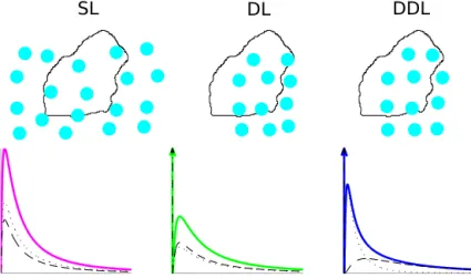
sub-component. The result is a delta-lognormal representa-tion of the hydrometeor fieldin each PDF component. Both delta functions are at zero and represent the region outside of precipitation, but the in-precipitation hydrometeor values are distributed as two lognormals that may have different means and/or variances. When the two lognormals differ in some way, the resulting distribution is called a delta-double-lognormal (DDL). Figure 1 illustrates the SL, DL, and DDL hydrometeor PDF shapes.
The main purpose of this paper is to present the formula-tion of an updated multivariate PDF that extends CLUBB’s traditional PDF to include the DL and DDL hydrometeor PDF shapes. Additionally, a new method is derived to divide the grid-box mean and variance of a hydrometeor species intoPDF componentmeans and standard deviations. A sec-ondary purpose of this paper is to present a preliminary com-parison of the new PDF shapes with PDF output by large-eddy simulations (LESs). The SL, DL, and DDL hydrom-eteor PDF shapes are compared to histograms of hydrome-teor data taken from precipitating LESs. Additionally, micro-physics process rates are calculated using each of the ideal-ized PDF shapes and compared to microphysics process rates taken from the LES.
The remainder of the paper is organized as follows. Sec-tion 2 gives a detailed descripSec-tion of the new PDF. SecSec-tion 3 discusses the PDF parameters and includes the derivation of a new method to divide the grid-box mean and variance into PDF component means and standard deviations for a hy-drometeor species. Section 4 describes the LES setup and the test cases, as well as the driving of CLUBB’s PDF for the tests. Section 5 presents a comparison of hydrometeors be-tween the LES and the SL, DL, and DDL PDF shapes. The comparison includes plots of PDFs, Kolmogorov–Smirnov and Cramer–von Mises scores, and microphysics process rates. Section 6 contains all conclusions.
2 Description of the multivariate PDF
We now describe how the multivariate PDF used by CLUBB is modified to improve the representation of hydrometeors. Perhaps the most important modification is the introduction of precipitation fraction,fp, to the PDF. Precipitation frac-tion is defined as the fracfrac-tion of the subgrid domain that contains any kind of precipitation (where any hydrometeor species has a positive value). In order to account for any precipitation-less region in the subgrid domain, the PDF is modified to add a delta function at a value of zero for all hydrometeor species. Each PDF component contains its own precipitation fraction. Expressed generally for a PDF of n
components, the overall precipitation fraction is related to the component precipitation fractions by
fp=
n X
i=1
DL DDL SL
Figure 1.A schematic of the single lognormal (SL), delta-lognormal (DL), and delta-double-lognormal (DDL) hydrometeor PDF shapes. The SL PDF shape is precipitating over the entire subgrid domain, whereas the DL and DDL shapes are not. In all three plots of the PDFs (where each PDF is a function of a hydrometeor species, such asrr), the weighted PDF from each PDF component is shown (black dashes and black dots). The sum of the two are the SL (solid magenta), the DL (solid green), and the DDL (solid blue). The SL does not contain a delta at 0, and the mean and variance of each PDF component are the same. Each component of the DL has a delta at 0 (upward pointing black arrows on theyaxis). The sum of the two component deltas forms the DL’s delta at 0 (upward pointing green arrow). The mean and variance of each DL PDF component are the same within precipitation. Each component of the DDL also has a delta at 0 (upward pointing black arrows). The sum of the two component deltas forms the DDL’s delta at 0 (upward pointing blue arrow). The mean and/or variance differ between DDL PDF components within precipitation.
where fp(i) denotes precipitation fraction in the ith PDF
component, and where 0≤ fp(i)≤ 1 for allfp(i).
Addition-ally
n X
i=1
ξ(i)=1, (2)
whereξ(i)is the relative weight, or mixture fraction, of the
ith PDF component, and where 0< ξ(i)<1 for all ξ(i). A
PDF with more than one component requires that each PDF component have a mixture fraction.
Before writing the form of the multi-component PDF, we digress to discuss a special case, the cloud droplet concen-tration (per unit mass), Nc. In Larson and Griffin (2013), Ncwas introduced to the PDF and was assumed to follow a single lognormal distribution. This assumption forNcmeans that when any cloud is found at a grid level,Nc>0 at every point on the subgrid domain. This is unphysical in a partly cloudy situation, because cloud droplets would be found at points where cloud water is not found. Additionally, the sin-gle lognormal treatment ofNccan cause problems with the microphysics. The grid-level mean of Nc, denotedNc (for the remainder of this paper, an overbar denotes a grid-level mean and a prime denotes a turbulent value), is handed to the PDF by the model, and this mean value includes clear air in a partly cloudy situation. This results in a value ofNcthat is much smaller than the in-cloud values ofNc. Since the sin-gle lognormal inNcis distributed aroundNc,Ncis much too small in cloud for cases with small cloud fraction, leading to an excessive autoconversion (raindrop formation) rate.
In order to distributeNcwhere (and only where) cloud wa-ter mixing ratio,rc, is found on the subgrid domain, it cannot use the same method as the other hydrometeors. Hydrome-teors such asrrcan be found outside clouds whererc is not found, or alternatively hydrometeors might be absent inside cloud wherercis found. Instead the PDF is modified so that a new variable,Ncn, replacesNc in the PDF. The variable Ncnis a mathematical construct that can be viewed as an ex-tended cloud droplet concentration or even as a simplified, conservative cloud condensation nuclei concentration. It is distributed as a single lognormal over the subgrid domain. At points where cloud water is found,Ncis set equal toNcn. Otherwise,Nc is set to 0 at points where no cloud water is found (see Eq. 4 below). The value ofNcnis approximately the in-cloud mean ofNc, and in special cases, is exactly the in-cloud mean ofNc. Please see Appendix B for a more de-tailed explanation.
The PDF includes all the hydrometeor species found in the chosen microphysics scheme with the exception of rc, which is calculated from other variables in the PDF through a saturation adjustment, andNc, which is described above. In addition torrandNr, a microphysics scheme may include hydrometeor species such as ice mixing ratio,ri, ice crys-tal concentration (per unit mass),Ni, snow mixing ratio,rs, snowflake concentration (per unit mass),Ns, graupel mix-ing ratio,rg, and graupel concentration (per unit mass),Ng. The vector containing all the hydrometeor species included in the PDF will be denotedh. The full PDF can be written as
In order to calculate quantities that depend on saturation, such as rc and cloud fraction, a PDF transformation is re-quired. The PDF transformation is a change of coordinates. The multivariate PDF undergoes translation, stretching, and rotation of the axes (Larson et al., 2005; Mellor, 1977). Within each PDF component, a separate PDF transformation takes place. Theith component PDF,P(i)(w, rt, θl, Ncn,h), is transformed to P(i)(w, χ , η, Ncn,h), where χ is an “ex-tended” liquid water mixing ratio that, when the air is su-persaturated, has a positive value and furthermore is equal to
rc. When the air is subsaturated,χhas a negative value. The variableη is orthogonal toχ. The variablesrc andNc can now be written as
rc=χ H (χ )and (3)
Nc=NcnH (χ ) , (4)
whereH (x)is the Heaviside step function.
The general form of a PDF withncomponents andD vari-ables (whetherDincludes all the variables in the PDF or any subset of those variables in a multivariate marginal PDF) can be written as
P (x1, x2, . . ., xD)= n X
i=1
ξ(i)P(i)(x1, x2, . . ., xD) . (5)
Of theDvariables listed, the firstJ variables are normally distributed in each PDF component (i.e.,w,rt, andθl, orw,χ andη), the nextKvariables are lognormally distributed (i.e.,
Ncn), and the lastvariables are the hydrometeor species, such that D=J+K+. The ith component of the PDF,
P(i)(x1, x2, . . ., xD), accounts for both the precipitating and
precipitation-less regions, and is given by
P(i)(x1, x2, . . ., xD)=
fp(i)P(J,K+)(i)(x1, x2, . . ., xD) (6)
+ 1−fp(i)
P(J,K)(i)(x1, x2, . . ., xJ+K) D Y
ǫ=J+K+1
δ (xǫ) !
.
The subscripts in theith component,P(J,K)(i)orP(J,K+)(i),
denote the number of normal variates,J, and the number of lognormal variates,KorK+, used in Eq. (7).
Each original PDF component is split into precipitat-ing and precipitation-less sub-components. The component means, variances, and correlations for variables x1. . .xJ+K
do not differ between the precipitating and precipitation-less parts of Eq. (6). This greatly simplifies the procedure for parameterizing the component means and variances, given the grid-level means and variances. Additionally, keeping the component means and variances the same between the in-precipitation and outside-in-precipitation parts of Eq. (6) allows the PDF to be reduced back to prior versions. For instance, the multivariate PDF in Eqs. (5) and (6) reduces to the ver-sion given in Larson and Griffin (2013) when all fp(i)=1
and various PDF parameters are chosen appropriately. Fur-thermore, when microphysics is not used in a simulation, hy-drometeors are not found in the PDF. In this scenario, the PDF reduces to the original version found in Golaz et al. (2002a).
The PDF does not contain a fraction for each hydrom-eteor species or type, but rather one precipitation fraction. Each PDF component is split into two sub-components (in-precipitation and outside-(in-precipitation). Including a fraction for each hydrometeor type (rain, snow, etc.) would cause the number of sub-components to grow exponentially with the number of fractions. Usingnfhydrometeor fractions in-creases the number of sub-components to 2nf in each PDF component. This would make setting the PDF parameters as-sociated with each sub-component increasingly difficult.
The multivariate PDF can be adjusted to account for a situation when a variable has a constant value in a PDF (sub-)component. In that situation, the variable can be re-duced to a delta function at the (sub-)component mean value. A good example of this would be settingNcnto a constant value in order to use a constant in-cloud value of cloud droplet concentration. This is also especially useful when dealing with more than one hydrometeor. If one hydrome-teor species is found at a grid level, but another hydromehydrome-teor species is not found at that level, the hydrometeor that is not found can reduce to a delta function at zero in the precipitat-ing sub-component of Eq. (6).
The general form of the m-variate hybrid nor-mal/lognormal distribution in the ith PDF component,
P(j,k)(i)(x1, x2, . . ., xm), which is found in each
sub-component of Eq. (6), consists ofj normal variates and k
lognormal variates, wherem=j+k. The firstj variables are normally distributed and the remainingk variables are lognormally distributed. The multivariate normal/lognormal PDF is given by (Fletcher and Zupanski, 2006)
P(j,k)(i)(x1, x2, . . ., xm)=
1
(2π )m26(i) 1 2
m Y
τ=j+1 1
xτ !
×exp
−1
2 x−µ(i)
T
6−(i)1 x−µ(i)
. (7)
Bothx andµ(i) are m×1 vectors, wherex is a vector of the variables (in normal-space) in the PDF andµ(i)is a vec-tor of the (normal-space) PDF sub-component means. The notation T denotes the transpose of the vector. Them×m
(normal-space) covariance matrix is denoted6(i)and its
de-terminant is denoted6(i)
(Fletcher and Zupanski, 2006). The advantage of asinglemultivariate PDF, as opposed to a collection of individual marginal PDFs, is that the multivari-ate PDF accounts for correlations among the variables in the PDF. This is advantageous when calculating quantities such as rain water accretion rate and rain water evaporation rate.
two variables at the same grid level, the PDF does not contain information about vertical correlations. Vertical correlations can arise in calculations of radiative transfer, diagnosed hy-drometeor sedimentation, or other processes that involve the correlation of a variable with itself at different vertical levels. Such processes are excluded from this study, and hence in-formation about vertical correlations is not needed here. For one possible method to parameterize vertical correlations, see Larson and Schanen (2013).
When variables are integrated out of the full multivariate PDF, the result is a multivariate marginal PDF consisting of fewer variables. When all variables but one are integrated out of the PDF, the result is a univariate marginal or individual marginal PDF. For any hydrometeor species,h, found in the full multivariate PDF in Eq. (5), the univariate marginal dis-tribution is
P (h)=
n X
i=1
ξ(i) fp(i)PL(i)(h)+ 1−fp(i)
δ (h), (8)
where PL(i)(h) is a lognormal distribution in the ith PDF
component, which is given by
PL(i)(h)=
1
(2π )12eσh(i) h exp
(
−lnh−eµh(i) 2
2eσh(i)2 )
. (9)
The in-precipitation mean ofhin theith PDF component isµh(i). This is the mean of theith lognormal ofh. However, e
µh(i), as in Eq. (9), is the normal-space component mean of
h. It is the in-precipitation mean of lnhin theith PDF com-ponent and is given by
e µh(i)=ln
µh(i) 1+
σh(i)2
µ2h(i) !−12
, (10)
whereσh(i)is the in-precipitation standard deviation ofhin
the ith PDF component. The quantity σh(i) is the standard
deviation of theith lognormal ofh. The normal-space com-ponent standard deviation ofh iseσh(i), as found in Eq. (9).
It is the in-precipitation standard deviation of lnhin theith PDF component and is given by
e σh(i)=
v u u
tln 1+σh(i)2
µ2h(i) !
. (11)
The variables that are distributed marginally as binormals use similar notation. For example, µw(i) is the mean ofw
in the ith PDF component, or the mean of theith normal. Likewise,σw(i)is the standard deviation ofwin theith PDF
component, or the standard deviation of theith normal.
3 PDF parameters
This paper will use the phrase “PDF parameters” to refer to the PDFcomponentmeans, standard deviations, and correla-tions involving variables in the PDF, as well as the mixture
fractions and the PDF component precipitation fractions. The PDF parameters are calculated from various grid-mean in-put variables. In this paper, the component means, standard deviations, and correlations involvingw,rt, andθl, and the mixture fractions,ξ(1) andξ(2), are calculated according to
the Analytic Double Gaussian 2 (ADG2) PDF, as described in Sect. (e) of the Appendix of Larson et al. (2002). ADG2 requires the following quantities as input: the overall (grid-box) mean, variance, and third-order central moment of w
(w,w′2, andw′3, respectively), the overall mean and vari-ance ofrt(rtandrt′2, respectively), and the overall mean and variance ofθl(θlandθl′
2
, respectively). ADG2 preserves the values of these input variables, meaning that the PDF param-eters can be used to successfully reconstruct the values of the input variables. Additionally, ADG2 requires and preserves the overall covariance ofwandrt(w′rt′), the overall covari-ance ofwandθl(w′θl′), and the overall covariance ofrtand θl(rt′θl′). All of the aforementioned quantities are prognosed or diagnosed in CLUBB and are not the subject of this paper. The individual marginal distribution forNcnis specified to be a single lognormal over the entire subgrid domain. This requires that both PDF component means equal the over-all (grid-box) mean (µNcn(1)=µNcn(2)=Ncn). Likewise, this requires that both PDF component standard deviations equal the overall standard deviation (σNcn(1)=σNcn(2)=Ncn′ 2
1/2 ). When no hydrometeor species are found at a grid level (h=0),fp=fp(1)=fp(2)=0. Otherwise, if any
hydrome-teor species inhis found at a grid level (has a value greater than 0), fp
tol≤fp≤1, where fp
tolis the minimum value allowed for precipitation fraction when hydrometeors are present. We now describe how CLUBB parameterizesfp(1)
andfp(2), givenfp. First, we note that
fp=ξ(1)fp(1)+ξ(2)fp(2). (12)
A tunable parameter,υ∗(where the∗subscript denotes a tun-able or adjusttun-able parameter), is introduced and is defined as the ratio ofξ(1)fp(1)tofp, where 0≤υ∗≤1. The precipita-tion fracprecipita-tion of PDF component 1 is solved by
fp(1)=min
υ
∗fp ξ(1)
,1
. (13)
The precipitation fraction of PDF component 2 can now be solved by
fp(2)=min
f
p−ξ(1)fp(1)
ξ(2)
,1
. (14)
Whenfp(1)calculated by Eq. (13) is small enough to force
fp(2) calculated by Eq. (14) to be limited at 1, the value of
fp(1)is recalculated (withfp(2)=1) and is increased enough
3.1 Hydrometeor PDF parameters
A mean-and-variance-preserving method is used to calculate the in-precipitation means of the hydrometeor field in the two PDF components, µh(1) andµh(2), and the in-precipitation
standard deviations of the hydrometeor field in the two PDF components,σh(1) andσh(2). The fields that need to be
pro-vided as inputs are the overall (grid-box) mean of the hy-drometeor,h, the overall variance of the hydrometeor,h′2
, the mixture fraction in each PDF component, ξ(1) andξ(2),
the overall precipitation fraction, fp, and the precipitation fraction in each PDF component,fp(1)andfp(2). Given these
inputs, the in-precipitation mean of the hydrometeor, h|ip, can be calculated by
h|ip= h fp
, (15)
and the in-precipitation variance of the hydrometeor, h|′ip2, can be calculated by
h|′ip2=h
′2
+h2−fph|ip 2
fp
. (16)
The grid-level mean value of any function that is written in terms of variables involved in the PDF can be found by integrating over the product of that function and the PDF. For example,
h=
∞
Z
0
h P (h)dh and
h′2 =
∞
Z
0
h−h2P (h)dh. (17)
After integrating, the equation for h expressed in terms of PDF parameters is
h=ξ(1)fp(1)µh(1)+ξ(2)fp(2)µh(2). (18)
Likewise, the equation for h′2
expressed in terms of PDF parameters is
h′2
=ξ(1)fp(1)
µ2h(1)+σh(21)
+ξ(2)fp(2)
µ2h(2)+σh(22)
−h2. (19)
When the hydrometeor is not found at a grid level, h= h′2
=0 and thecomponentmeans and standard deviations of the hydrometeor also have a value of 0. When the hydrom-eteor is found at a grid level, h >0. Precipitation may be found in only PDF component 1, only PDF component 2, or in both PDF components. When precipitation is found in only
PDF component 1,µh(2)=σh(2)=0 andµh(1)andσh(1)can
easily be solved by Eqs. (18) and (19). Likewise, when pre-cipitation is found in only PDF component 2,µh(1)=σh(1)=
0 andµh(2)andσh(2)can easily be solved by the same
equa-tion set.
When there is precipitation found in both PDF compo-nents, further information is required to solve for the two component means and the two component standard devia-tions. The variableRis introduced such that
R≡ σ
2
h(2)
µ2h(2). (20)
In order to allow the ratio ofσh(21) toµ2h(1) to vary, the pa-rameterζ∗is introduced, such that
R (1+ζ∗)= σh(21)
µ2h(1), (21)
whereζ∗>−1. Whenζ∗>0, thenσh(21)/µ2h(1) increases at the expense ofσh(22)/µ2h(2), which decreases in this variance-preserving equation set. When ζ∗=0, then σh(21)/µ2h(1)= σh(22)/µ2h(2). When−1< ζ∗<0, thenσh(22)/µ2h(2) increases at the expense ofσh(21)/µ2h(1), which decreases. Combining Eqs. (19), (20), and (21), the equation forh′2can be rewrit-ten as
h′2
=ξ(1)fp(1)(1+R (1+ζ∗)) µ2h(1)
+ξ(2)fp(2)(1+R) µ2h(2)−h
2
. (22)
Both the variance of each PDF component and the spread between the means of each PDF component contribute to the in-precipitation variance of the hydrometeor (h|′ip2). At one extreme, the standard deviation of each component could be set to 0 and the in-precipitation variance could be accounted for by spreading the PDF component (in-precipitation) means far apart. The value ofRin this scenario would be its minimum possible value, which is 0. At the other extreme, the means of each component could be set equal to each other and the in-precipitation variance could be ac-counted for entirely by the PDF component (in-precipitation) standard deviations. The value ofRin this scenario would be its maximum possible value, which isRmax.
In order to calculate the value ofRmax, setµh(1)=µh(2)=
h|ipandR=Rmax. Eq. (22) becomes h′2
+h2=h|ip2 ξ(1)fp(1)(1+Rmax(1+ζ∗))
+ξ(2)fp(2)(1+Rmax). (23) When Eq. (16) is substituted into Eq. (23),Rmaxis solved for and the equation is
Rmax=
f
p
ξ(1)fp(1)(1+ζ∗)+ξ(2)fp(2) h|′
ip 2
h|ip
In the scenario thatζ∗=0 the equation forRmaxreduces to the ratio of h|′ip2to h|ip
2 .
In order to calculate the value of R, a parameter is used to prescribe the ratio ofRto its maximum value,Rmax. The prescribed parameter is denotedo∗, where
R=o∗Rmax, (25)
and where 0≤o∗≤1. BothR and Rmax are known func-tions of the inputs and tunable parameters. Wheno∗=0, the standard deviation of each PDF component is 0, andµh(1)
is spread far from µh(2). Wheno∗=1, thenµh(1)=µh(2),
and the standard deviations of the PDF components account for all of the in-precipitation variance. At intermediate val-ues ofo∗, the means of each PDF component are somewhat spread apart and each PDF component has some width. The new equation for hydrometeor variance becomes
h′2
=ξ(1)fp(1)(1+o∗Rmax(1+ζ∗)) µ2h(1)
+ξ(2)fp(2)(1+o∗Rmax) µ2h(2)−h
2
. (26)
The two remaining unknowns, µh(1) and µh(2), can be
solved by a set of two equations, Eq. (18) forhand Eq. (26) for h′2. All other quantities in the equation set are known quantities. To find the solution, Eq. (18) is rewritten to iso-lateµh(2)such that
µh(2)=
h−ξ(1)fp(1)µh(1)
ξ(2)fp(2)
. (27)
The above equation is substituted into Eq. (26). The resulting equation is rewritten in the form
Qaµ2h(1)+Qbµh(1)+Qc=0, (28)
so the solution to the quadratic equation forµh(1)is
µh(1)=
−Qb± q
Q2b−4QaQc
2Qa
, (29)
where
Qa=ξ(1)fp(1)(1+o∗Rmax(1+ζ∗)) +
ξ(21)fp2(1)
ξ(2)fp(2)
(1+o∗Rmax) ,
Qb= −2
ξ(1)fp(1)
ξ(2)fp(2)
(1+o∗Rmax) h, and
Qc= −
h′2 +
1−1+o∗Rmax ξ(2)fp(2)
h2
. (30)
The value of Qa is always positive and the value ofQb is
always negative. The value ofQccan be positive, negative,
or zero. Since 1−(1+o∗Rmax) / ξ(2)fp(2)
h2 is always
negative andh′2is always positive, the sign ofQ
cdepends
on which term is greater in magnitude. When h′2 is greater, the sign of Q
c is negative. This
means that−4QaQc is positive, which in turn means that q
Q2b−4QaQcis greater in magnitude than−Qb. If the
sub-traction option of the±were to be chosen, the value ofµh(1)
would be negative in this scenario. At first glance, it might appear natural to always choose the addition option. How-ever, this set of equations was derived with the condition that
µh(1) equalsµh(2)wheno∗=1. Whenζ∗≥0, this happens
when the addition option is chosen, but not when the sub-traction option is chosen. However, whenζ∗<0, this hap-pens when the subtraction option is chosen, but not when the addition option is chosen. So, the equation forµh(1)becomes
µh(1)=
−Qb+ q
Q2b−4QaQc
2Qa
, whenζ∗≥0; and
−Qb− q
Q2b−4QaQc
2Qa
, whenζ∗<0.
(31) The value ofµh(2) can now be found using Eq. (27).
Af-terµh(1) andµh(2)have been solved,σh(1)andσh(2)can be
solved by plugging Eq. (25) back into Eqs. (21) and (20), respectively.
As the value of h|′ip2/ h|ip 2
increases and as the value of
o∗decreases (narrowing the in-precipitation standard devia-tions and increasing the spread between the in-precipitation means), one of the component means may become negative. This happens because there is a limit to the amount of in-precipitation variance that can be represented by this kind of distribution. In order to prevent out-of-bounds values of
µh(1)orµh(2), a lower limit is declared, called µh|min, where µh|minis a small, positive value that is typically set to be 2 orders of magnitude smaller than h|ip. The value ofµh(1)or
µh(2) will be limited from becoming any smaller (or
nega-tive) at this value. From there, the value of the other hydrom-eteor in-precipitation component mean is easy to calculate. Then, both values will be entered into the calculation of hy-drometeor variance in Eq. (22), which will be rewritten to solve forR. Then, both the hydrometeor mean and hydrom-eteor variance will be preserved with a valid distribution.
When the value ofζ∗≥0, the value ofµh(1) tends to be
larger than the value ofµh(2). Likewise when the value of
ζ∗<0, the value of µh(2) tends to be larger than the value
ofµh(1). Since most cloud water and cloud fraction tends to
be found in PDF component 1, it is appropriate and advanta-geous to have the larger in-precipitation component mean of the hydrometeor also found in PDF component 1. The rec-ommended value ofζ∗is a value greater than or equal to 0.
0< o∗<1 or whenζ∗6=0. The DL hydrometeor PDF shape is produced simply by settingo∗=1 andζ∗=0. These set-tings forceµh(1)=µh(2)andσh(1)=σh(2), which result in a
single lognormal within the precipitating portion of the sub-grid domain. Furthermore, if, in addition to setting o∗=1 andζ∗=0, one simply setsfp(1)=fp(2)=1, then
precipita-tion is found everywhere within the subgrid domain, produc-ing the SL hydrometeor PDF shape. Hence, it is very easy to change between DDL, DL, and SL hydrometeor PDF shapes. Additionally, it should be noted that there is only oneo∗and only oneζ∗applied to all the hydrometeor species inh.
In limited testing, the value of the tunable parameterζ∗did not affect the results much for CLUBB’s DDL PDF shape. The value of ζ∗ has been left at 0, effectively eliminating a tunable or adjustable parameter from the scheme. When
ζ∗=0, the DDL shape approaches the DL shape aso∗ ap-proaches 1. Aso∗approaches 0, the DDL shape approaches a double delta in precipitation (in addition to the delta at 0). Additionally, when 0< o∗<1, the in-precipitation skew-ness of the hydrometeor field is influenced byυ∗. Asυ∗ ap-proaches 0, the in-precipitation distribution becomes more highly (positively) skewed. In Gaussian space (see Sect. 5), the in-precipitation distribution is positively skewed. Asυ∗
approaches 1, the in-precipitation distribution is less (posi-tively) skewed. In Gaussian space, the in-precipitation distri-bution is negatively skewed. For the results presented in this paper for the DDL hydrometeor PDF shape, the remaining two tunable parameters have been set to the valueso∗=0.5 andυ∗=0.55.
4 Model setup and testing
There is insufficient data from observations to calculate all the fields that need to be input into CLUBB’s PDF. However, this data can be supplied easily and plentifully by a LES. In this paper, LES output of precipitating cases is simulated by the System for Atmospheric Modeling (SAM) (Khairoutdi-nov and Randall, 2003). SAM uses an anelastic equation set that predicts liquid water static energy, total water mixing ra-tio, vertical velocity, and both the south–north and west–east components of horizontal velocity. Additionally, it predicts hydrometeor fields as directed by the chosen microphysics scheme. A predictive 1.5-order subgrid-scale turbulent ki-netic energy closure is used to compute the subgrid-scale fluxes (Deardorff, 1980). SAM uses a fixed, Cartesian spa-tial grid and a third-order Adams–Bashforth time-stepping scheme to advance the predictive equations of motion. It uses periodic boundary conditions and a rigid lid at the top of the domain. The second-order MPDATA (multidimensional positive definite advection transport algorithm) scheme is used to advect the predictive variables (Smolarkiewicz and Grabowski, 1990).
In order to assess the generality of the different hydrome-teor PDF shapes for different cloud regimes, SAM was used
to run three idealized test cases – a precipitating shallow cu-mulus case, a drizzling stratocucu-mulus case, and a deep con-vective case. The use of cases from differing cloud regimes help avoid overfitting the parameterizations of PDF shape. The setup for the precipitating shallow cumulus test case was based on the Rain in Cumulus over the Ocean (RICO) LES intercomparison (van Zanten et al., 2011). The horizontal res-olution was 100 m, and 256 grid boxes were used in each hor-izontal direction. The vertical resolution was a constant 40 m and 100 grid boxes were used in the vertical. The model top was located at 4000 m in altitude. The model time step was 1 s and the duration of the simulation was 72 h. A vertical profile of level-averaged statistics was output every minute and a three-dimensional snapshot of hydrometeor fields was output every hour.
The RICO simulation was run with SAM’s implementa-tion of the Khairoutdinov and Kogan (2000, hereafter KK) warm microphysics scheme. KK microphysics predicts both
rrandNr. SAM’s implementation of KK microphysics uses a saturation adjustment to diagnoserc, and cloud droplet con-centration is set to a constant value (which is 70 cm−3 for RICO).
The setup for the drizzling stratocumulus test case was taken from the LES intercomparison based on research flight 2 (RF02) of the second Dynamics and Chemistry of Ma-rine Stratocumulus (DYCOMS-II) field experiment (Acker-man et al., 2009). The horizontal resolution was 50 m and 128 grid boxes were used in each horizontal direction. An unevenly spaced vertical grid was used containing 96 grid boxes and covering a domain of depth 1459.3 m. The model time step was 0.5 s and the duration of the simulation was 6 hours. A vertical profile of level-averaged statistics was out-put every minute and a three-dimensional snapshot of hy-drometeor fields was output every 30 min. The DYCOMS-II RF02 simulation was also run with SAM’s implementation of KK microphysics and used a constant cloud droplet con-centration of 55 cm−3.
The setup for the deep convective test case was taken from the LES intercomparison based on the Large-Scale Biosphere–Atmosphere (LBA) experiment (Grabowski et al., 2006). The horizontal resolution was 1000 m, and 128 grid boxes were used in each horizontal direction. An unevenly spaced vertical grid was used, containing 128 grid boxes and covering a domain of depth 27 500 m. The model time step was 6 s and the duration of the simulation was 6 hours. A vertical profile of level-averaged statistics was output ev-ery minute and a three-dimensional snapshot of hydrometeor fields was output every 15 min for the final 3.5 h of the simu-lation.
us-ing a saturation adjustment right before the microphysics is called and then allows microphysics to update the value of
rc, which in turn is used to update the valuert. Cloud droplet concentration was set to a constant value of 100 cm−3.
CLUBB’s hydrometeor PDF shapes will be compared to histograms of hydrometeors produced by SAM LES data. Our goal is to isolate errors in the PDF shape itself. In order to eliminate sources of error outside of the PDF shape and provide an “apples-to-apples” comparison of CLUBB’s PDF shapes to SAM data, we drive CLUBB’s PDF using SAM LES fields, rather than perform interactive CLUBB simula-tions. The following fields are taken from SAM’s statistical profiles and are used as inputs to CLUBB’s PDF:rt,θl,w′2, rt′2,θl′2,w′r′
t,w′θl′,rt′θl′,w′ 3
,fp,rr,rr′2,Nr, andNr′2. For the LBA case, we addri,ri′2,Ni,Ni′2,rs,rs′2,Ns,Ns′2,rg, r′
g2,Ng, andNg′2. Another input to CLUBB’s PDF isw. The value ofwfrom large-scale forcing is set according to case specifications in both SAM and CLUBB. CLUBB’s PDF is generated at every SAM vertical level and at every output time of SAM level-averaged statistical profiles.
Additionally, covariances that involve at least one hydrom-eteor are added to the above list and are used to calculate the PDF component correlations of the same two variables. These covariances arert′r′
r,θl′rr′,rt′Nr′,θl′Nr′, andrr′Nr′. Please see Appendix A for more details on the calculation of PDF component correlations. The values of the component cor-relations do not affect the individual marginal PDFs of the hydrometeors. They are included for the calculation of mi-crophysics process rates (see Sect. 5.2).
Owing to differences between the KK and Morrison mi-crophysics schemes in SAM, fpused by CLUBB’s PDF is computed slightly differently depending on which micro-physics scheme is used by SAM. The differences are due to the number of hydrometeor species involved in the mi-crophysics, the thresholding found internally in the micro-physics codes, and the variables that are output to statistics by SAM. KK microphysics contains only rain, and SAM’s im-plementation of KK microphysics clips any value ofrr(and with itNr) below a threshold value in clear air. Therefore, it is simple to setfpto the fraction of the domain occupied by non-zero values ofrrandNr. Morrison microphysics predicts rain, ice, snow, and graupel. For each of these species, SAM outputs a fraction. To provide an apples-to-apples compari-son with CLUBB,fpis approximated as the greatest of these four fractions at any particular grid level.
Althoughfpis provided by the LES for this study, it can be diagnosed based on the cloud fraction using a method such as that of Morrison and Gettelman (2008). If the cloud fraction, in turn, is diagnosed based on the omnipresent prediction of means, variances, and other moments – as in higher-order moment parameterizations such as CLUBB – then the onset of partial cloudiness is well defined and indeterminacy about the time of cloud initiation is avoided. In contrast,
parame-terizations that diagnose cloud fraction based on, e.g., cloud water mixing ratio, lack crucial information in cloudless grid boxes, as discussed in Tompkins (2002). The well-defined onset of CLUBB’s cloud fraction is inherited by the precipi-tation fraction.
5 Results
We first evaluate the shape of the idealized PDFs directly against SAM LES output data. Histograms of SAM LES data are generated from the three-dimensional snapshots of hy-drometeor fields. One histogram is generated at every verti-cal level for each hydrometeor field. A histogram of a SAM hydrometeor field is compared to the CLUBB marginal PDF of that hydrometeor field at the same vertical level and output time. The comparison is done with each of the SL, DL, and DDL PDF shapes.
Figure 2 compares marginal PDFs involvingrrandNrfor the RICO case at an altitude of 380 m and a time of 4200 min. For the plot of the PDF ofrr in Fig. 2a, the delta function atrr=0 has been omitted. The SAM data are divided into 100 bins, equally sized inrr, that range from the largest value of rr to the smallest positive value of rr. (In what follows, all histograms use 100 equal-size bins, arranged from small-est to largsmall-est value.) The SL hydrometeor PDF shape signif-icantly overpredicts the PDF at small values ofrrand signif-icantly underpredicts it at large values ofrr. These errors are an expected consequence of the single lognormal’s attempt to fit the precipitation-less area. The DL and DDL PDF shapes provide a much closer match qualitatively to the SAM data. A quantitative assessment of the quality of the fit will follow in Sect. 5.1.
Each of the CLUBB hydrometeor PDF shapes has a log-normal distribution within precipitation in each PDF compo-nent. Taking the natural logarithm of every point of a lognor-mal distribution produces a norlognor-mal distribution, and so the plot of the PDF of lnrrin Fig. 2b is a normal distribution in each PDF component for each of the DDL, DL, and SL PDF shapes. The plot of the PDF of lnrr(hereafter referred to as the PDF ofrrin Gaussian space) complements the aforemen-tioned plot of the PDF ofrr(Fig. 2a). The plot of the PDF of rr is log-scaled on they axis, accentuating the small values ofP (rr)that are found at large values ofrr. The plot of the PDF of lnrraccentuates the PDF at small values ofrr.
The plot of the PDF of lnrr is a plot of only the in-precipitation portion of the distribution, omitting all zero-values. The in-precipitation portion of the PDF is divided byfp, which allows the area under the curve to integrate to 1. The PDF shown in Fig. 2b is the Gaussianized form of Eq. (32).
con-0 0.5 1 1.5 2 2.5 x 10⁻³ 10−1
100 101 102 103
r
r [kg kg
−1]
P( r
r
)
RICO: Rain water mixing ratio, r
r
LES DDL DL SL (a)
−18 −16 −14 −12 −10 −8 −6 0
0.05 0.1 0.15 0.2 0.25 0.3
ln rr [ln(kg kg−1)]
P(
ln
r r
)
| ip
RICO: Natural log of rain water mixing ratio, ln rr
LES DDL DL SL (b)
0 2 4 6 8 10
x 104 10−8
10−7 10−6 10−5 10−4
N
r [kg
−1
]
P( N
r
)
RICO: Rain drop concentration, Nr
LES DDL DL SL (c)
0 2 4 6 8 10
0 0.05 0.1 0.15 0.2 0.25 0.3 0.35
ln N
r [ln(kg
−1)]
P(
ln
N r
)
| ip
RICO: Natural log of rain drop concentration, ln Nr
LES DDL DL SL (d)
Figure 2.PDFs of rain in the RICO precipitating shallow cumulus case at an altitude of 380 m and a time of 4200 min. The SAM LES results are in red, the DDL results are blue solid lines, the DL results are green dashed lines, and the SL results are magenta dashed-dotted lines.
(a)The marginal distribution ofrrwith the delta atrr=0 omitted.(b)The marginal distribution of lnrrusing the “in-precipitation PDF”. This is the in-precipitation marginal PDF in Gaussian space.(c)The marginal distribution ofNrwith the delta atNr=0 omitted.(d)The marginal distribution of lnNrusing the “in-precipitation PDF”. Again, this is the in-precipitation marginal PDF in Gaussian space. The DDL provides a better fit to SAM LES than the DL, which in turn provides a better fit than the SL.
tinuous PDF shape that tries to include a delta function at zero. The DL PDF shape is far too peaked in comparison to the SAM LES data, which is spread out broadly in Gaussian space. The DDL PDF shape is able to achieve a spread-out shape because it has two different means within precipita-tion. This allows it to better fit the more platykurtic shape of the SAM LES data in Gaussian space.
The plot of the PDF of RICO Nris found in Fig. 2c and the Gaussian-space plot ofNris found in Fig. 2d. Similar to rr, the SL shape overpredicts the PDF at small values ofNr and underpredicts it at large values ofNr. In Gaussian space, it is easy to see that SL’s peak is located too far to the left. The DDL shape provides a better fit than the DL shape to SAM LES data in Fig. 2c. Again, the DL shape is too peaked in Fig. 2d, whereas the bimodal DDL is able to spread out, which provides a better match to SAM LES data.
Figure 3 contains scatter plots that show the bivariate PDF ofrrandNrfor both SAM LES and CLUBB’s PDF in RICO at the same altitude and time as Fig. 2. The CLUBB PDF scatter points were generated by sampling the DDL PDF using an unweighted Monte Carlo sampling scheme. This
demonstrates the advantages of the multivariate nature of CLUBB’s PDF. The hydrometeor fields are correlated the same way in CLUBB’s PDF as they are in SAM LES.
Figure 4 compares marginal PDFs involvingrrandNrfor the DYCOMS-II RF02 case at an altitude of 400 m and a time of 330 min. All three hydrometeor PDF shapes provide a decent match to the SAM LES data. In Fig. 4a and c, the SL and DL PDF shapes dip a little below the SAM LES line in the middle of the data range forrr andNr, respectively. The DDL PDF shape stays closer to the SAM LES line in this region. Additionally, the SL PDF shape overestimates the SAM LES line close to they axis. In Fig. 4b and d, the Gaussian-space plots show that the two components of the DDL shape superimpose more than they did for the RICO case, owing to the reduced in-precipitation variance in the drizzling stratocumulus case.
Figure 3.Joint PDF ofrrandNrin the RICO precipitating shallow cumulus case at an altitude of 380 m and a time of 4200 min. SAM LES results are the red scatter points. CLUBB PDF scatter points were generated by sampling the DDL PDF using an unweighted Monte Carlo scheme. The SAM LES domain is 256×256 grid points. So to provide for the best comparison of LES points to CLUBB PDF sample points, 65 536 CLUBB PDF sample points were used. The light blue scatter points are from PDF component 1 and the dark blue scatter points are from PDF component 2. Every 10th point was plotted from both SAM LES and CLUBB’s PDF. The joint nature of the PDF allowsrrand Nrto correlate the same way in CLUBB as they do in SAM.
330 min. Compared to SAM’s PDF, the DDL hydrometeor PDF shape is too bimodal, but it still provides the best visual match of the three hydrometeor PDF shapes to SAM data. The fit will be quantified in Sect. 5.1.
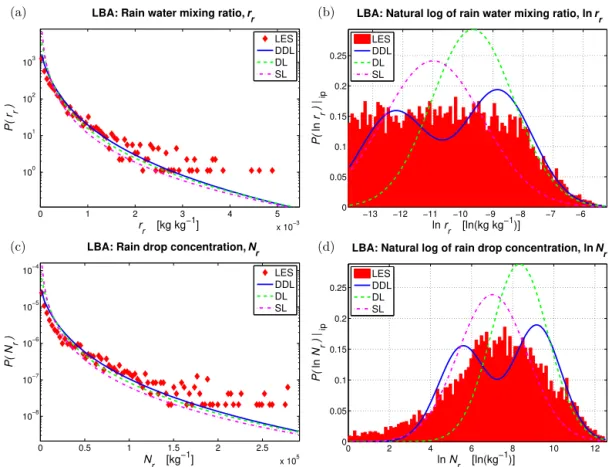
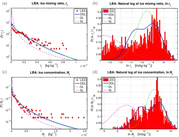
To indicate whether the three PDF shapes work for ice-phase hydrometeors, we compare marginal PDFs involvingri andNifor the LBA case at an altitude of 10 500 m and a time of 360 min (Fig. 6). Similar to therrandNrplots for RICO and LBA, Fig. 6a and c show that the SL PDF shape overpre-dicts the PDF at small values ofriandNiand underpredicts it at large values ofriandNi. The DL shape provides a better fit than the SL, and the DDL has a slightly better fit than the DL. The Gaussian-space plots in Fig. 6b and d show that the SAM LES distribution of lnriand lnNiis again platykurtic. The SL PDF shape has a peak that is shifted to the left. The DDL hydrometeor PDF shape is able to spread out the most to cover the platykurtic shape of the LES in Gaussian space. Why does the DDL PDF shape match LES output better than the DL shape in the aforementioned figures? The PDFs (in Gaussian space) for the LES of RICO and LBA show a broad, flat distribution of hydrometeor values from the LES. The DL shape is too peaked in comparison to the LES data. The DDL PDF is able to spread out the component means and thereby represent the platykurtic shape more accurately.
However, even the DDL PDF fails to capture the far left-hand tail of the LES PDF. In the RICO, DYCOMS-II RF02, and LBA cases, between about 5 and 20 % of the LES PDF is found to the left of the DDL PDF (see Figures 2b, 4b, 5b, and 6b). However, these values of hydrometeor mixing ratios are small. They are roughly a factor of 20 or more smaller than the median value. By combining these factors, we see that the percentage contribution of hydrometeor mixing ra-tios that are omitted on the left-hand tail is only about 1 %.
Why does SAM LES data have a platykurtic shape in Gaussian space in these cases? One possible cause is the partly cloudy (and partly rainy) nature of these cases. In these partly rainy cases, a relatively high percentage of the precipi-tation occurs in “edge regions” near the non-precipitating re-gion. These regions usually correspond to the edge of cloud or outside of cloud. Evaporation (or less accretion) occurs in these regions, increasing the area occupied by smaller amounts of rain. Yet, there is also an area of more intense pre-cipitation near the center of the precipitating region, which produces larger amounts of rain. Collectively, the areas of small and large rain amount produce the large spread in the hydrometeor spectrum.
0 0.2 0.4 0.6 0.8 1 1.2 1.4 1.6 x 10⁻⁴ 101
102 103 104
rr [kg kg−1]
P( r
r
)
RF02: Rain water mixing ratio, rr
LES DDL DL SL
(a)
−18 −16 −14 −12 −10
0 0.05 0.1 0.15 0.2 0.25 0.3 0.35 0.4 0.45
ln r
r [ln(kg kg
−1
)]
P(
ln
rr
)
| ip
RF02: Natural log of rain water mixing ratio, ln rr
LES DDL DL SL
(b)
0 2 4 6 8 10 12
x 104 10−8
10−7 10−6 10−5
N
r [kg
−1
]
P( N
r
)
RF02: Rain drop concentration, Nr
LES DDL DL SL
(c)
0 2 4 6 8 10
0 0.1 0.2 0.3 0.4 0.5
ln Nr [ln(kg−1)]
P(
ln
N r
)
| ip
RF02: Natural log of rain drop concentration, ln Nr
LES DDL DL SL
(d)
Figure 4.PDFs of rain in the DYCOMS-II RF02 drizzling stratocumulus case at an altitude of 400 m and a time of 330 min. The SAM LES results are in red, the DDL results are blue solid lines, the DL results are green dashed lines, and the SL results are magenta dashed-dotted lines.(a)The marginal distribution ofrrwith the delta atrr=0 omitted.(b)The marginal distribution of lnrrusing the “in-precipitation PDF.” This is the in-precipitation marginal PDF in Gaussian space.(c)The marginal distribution ofNrwith the delta atNr=0 omitted. (d)The marginal distribution of lnNrusing the “in-precipitation PDF”, which is the in-precipitation marginal PDF in Gaussian space. Owing to relatively low in-precipitating variance, the three hydrometeor PDF shapes are all a close match to SAM LES.
case is overcast, so there are not as many “edge” regions of precipitation as found in partly rainy cases. There is much less in-precipitation variance in the RF02 case. The simpler PDF shape is easier to fit by all the PDF shapes (SL, DL, and DDL). To further illuminate the physics underlying the PDF shapes produced by LESs, further study would be needed. 5.1 Quality of fit: general scores
While a lot can be learned by looking at plots of the hydrom-eteor PDFs, they are anecdotal and cannot tell us how well the idealized PDF shapes work generally. To obtain an over-all quantification of the quality of the fit, we calculate the Kolmogorov–Smirnov (K–S) and the Cramer–von Mises (C– vM) scores.
Both the K–S and C–vM tests compare the cumulative dis-tribution function (CDF) of the idealized disdis-tribution to the CDF of the empirical data (in this case, SAM LES data). Both tests require that the CDFs be continuous. Therefore, the scores are calculated using only the in-precipitation
por-tion of the hydrometeor PDF in Eq. (8). The DDL, DL, and SAM LES data all have the same precipitation fraction. The in-precipitation portion of the PDF is normalized by divid-ing by precipitation fraction so that it integrates to 1. The equation for the in-precipitation portion of the marginal PDF,
P (h)|ip, is
P (h)|ip=ξ(1)
fp(1)
fp
PL(1)(h)+ξ(2)
fp(2)
fp
PL(2)(h) , (32)
wherePL(i)is given by Eq. (9).
0 1 2 3 4 5 x 10⁻³ 100
101 102 103
r
r [kg kg
−1]
P( r
r
)
LBA: Rain water mixing ratio, r
r
LES DDL DL SL (a)
−13 −12 −11 −10 −9 −8 −7 −6 0
0.05 0.1 0.15 0.2 0.25
ln rr [ln(kg kg−1)]
P(
ln
r r
)
| ip
LBA: Natural log of rain water mixing ratio, ln rr
LES DDL DL SL (b)
0 0.5 1 1.5 2 2.5
x 105 10−8
10−7 10−6 10−5 10−4
N
r [kg
−1
]
P( N
r
)
LBA: Rain drop concentration, Nr
LES DDL DL SL (c)
0 2 4 6 8 10 12
0 0.05 0.1 0.15 0.2 0.25
ln N
r [ln(kg
−1)]
P(
ln
N r
)
| ip
LBA: Natural log of rain drop concentration, ln Nr
LES DDL DL SL (d)
Figure 5.PDFs of rain in the LBA deep convective case at an altitude of 2424 m and a time of 330 min. The SAM LES results are in red, the DDL results are blue solid lines, the DL results are green dashed lines, and the SL results are magenta dashed-dotted lines.(a)The marginal distribution ofrrwith the delta atrr=0 omitted.(b)The marginal distribution of lnrrusing the “in-precipitation PDF.” This is the in-precipitation marginal PDF in Gaussian space.(c)The marginal distribution ofNrwith the delta atNr=0 omitted.(d)The marginal distribution of lnNrusing the “in-precipitation PDF”, which is the in-precipitation marginal PDF in Gaussian space. Again, the DDL provides the best fit to SAM LES.
KS=max
h
Ce(h)|ip−C (h)|ip
=max KS+, KS−,where
KS+= max 1≤κ≤np
κ np−
C (hκ)|ip
and
KS−= max 1≤κ≤np
C (hκ)|ip− κ−1
np
.
(33) The number of data points in SAM LES where the hydrom-eteor is found is denoted np, andhκ is the value of the
hy-drometeor at SAM LES-ordered data pointκ.
Unlike the K–S test, which only considers the greatest dif-ference between the CDFs, the C–vM test is based on an in-tegral that includes the differences between the CDFs over the entire distribution. The integral is (Anderson, 1962)
ω2= Z
Ce(h)|ip−C (h)|ip 2
dC (h)|ip. (34)
The C–vM score is calculated by (Anderson, 1962; Stephens, 1970)
CVM=ω2np= 1 12np+
np
X
κ=1
2κ−1 2np −
C (hκ)|ip 2
0 0.2 0.4 0.6 0.8 1 x 10⁻³ 100
101 102 103 104
r
i [kg kg
−1
]
P( r
i
)
LBA: Ice mixing ratio, ri
LES DDL DL SL (a)
−13 −12 −11 −10 −9 −8 −7 0
0.05 0.1 0.15 0.2 0.25 0.3 0.35 0.4
ln r
i [ln(kg kg
−1
)]
P(
ln
r i
)
| ip
LBA: Natural log of ice mixing ratio, ln ri
LES DDL DL SL (b)
0 0.5 1 1.5 2 2.5
x 107 10−10
10−9 10−8 10−7
N
i [kg
−1
]
P( N
i
)
LBA: Ice concentration, Ni
LES DDL DL SL (c)
6 8 10 12 14 16
0 0.05 0.1 0.15 0.2 0.25 0.3 0.35 0.4
ln N
i [ln(kg
−1
)]
P(
ln
N i
)
| ip
LBA: Natural log of ice concentration, ln Ni
LES DDL DL SL (d)
Figure 6.PDFs of ice in the LBA deep convective case at an altitude of 10 500 m and a time of 360 min. The SAM LES results are in red, the DDL results are blue solid lines, the DL results are green dashed lines, and the SL results are magenta dashed-dotted lines.(a)The marginal distribution ofri with the delta atri=0 omitted.(b)The marginal distribution of lnriusing the “in-precipitation PDF.” This is the in-precipitation marginal PDF in Gaussian space.(c)The marginal distribution ofNiwith the delta atNi=0 omitted.(d)The marginal distribution of lnNiusing the “in-precipitation PDF.” Again, this is the in-precipitation marginal PDF in Gaussian space. The method works for frozen hydrometeor species as well, as the DDL provides a better fit to SAM LES than the DL, which in turn provides a better fit than the SL.
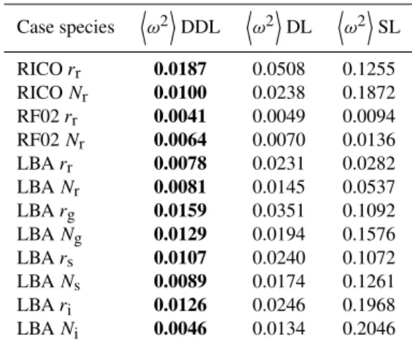
and output times, so the C–vM scores cannot simply be aver-aged. Rather, they are normalized first by dividing CVM by
npto produceω2 at every level and time. Those results are averaged to calculateω2.
After inspecting profiles of SAM LES results for mean mixing ratios in height and time, regions were identified in height and time where the mean mixing ratio of a species was always at least 5.0×10⁻⁶kg kg−1. Averaging of the scores was restricted to these regions in order to eliminate from consideration levels that do not contain the hydrome-teor or contain only small amounts of the hydromehydrome-teor with a small number of samples. RICO test scores for rr andNr were averaged from the surface through 2780 m and from 4200 through 4320 min. DYCOMS-II RF02 test scores forrr andNrwere averaged from 277 through 808 m and from 300 to 360 min.
The LBA case contains both liquid and frozen-phase hy-drometeor species that evolve as the cloud system transi-tions from shallow to deep convection. The various hydrom-eteor species develop and maximize at different altitudes and
times, so different periods and altitude ranges are chosen for averaging test scores for each species. LBA test scores forrr andNrwere averaged from the surface through 6000 m and from 285 through 360 min. The test scores forrgandNgwere averaged from 4132 through 9750 m and from 315 through 360 min. The test scores forrs andNs were averaged from 5026 m through 9000 m and from 345 through 360 min. Fi-nally, the test scores forriandNiwere averaged from 10 250 through 11 750 m at 360 min. For the LBA case, the value of
fpused by CLUBB’s PDF was based on the greatest value of SAM output variables for rain fraction, ice fraction, snow fraction, and graupel fraction. Each of these statistics is the fraction of the SAM domain occupied by values of the rele-vant mixing ratio of at least 1.0×10⁻⁶kg kg−1. In order to keep the comparison of the PDF shapes to SAM data consis-tent, values lower than this threshold were omitted from the calculations of the individual level-and-time scores for K–S and C–vM.
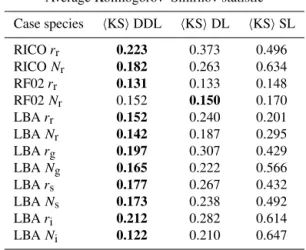
Table 1.Kolmogorov–Smirnov statistic averaged over multiple grid levels and statistical output timesteps comparing each of DDL, DL, and SL hydrometeor PDF shapes to SAM LES results. The best (lowest) average score for each case and hydrometeor species is listed in bold. The DDL has the lowest average score most often, and the DL has the second-lowest average score most often.
Average Kolmogorov–Smirnov statistic
Case species hKSiDDL hKSiDL hKSiSL
RICOrr 0.223 0.373 0.496
RICONr 0.182 0.263 0.634
RF02rr 0.131 0.133 0.148
RF02Nr 0.152 0.150 0.170
LBArr 0.152 0.240 0.201
LBANr 0.142 0.187 0.295
LBArg 0.197 0.307 0.429
LBANg 0.165 0.222 0.566
LBArs 0.177 0.267 0.432
LBANs 0.173 0.238 0.492
LBAri 0.212 0.282 0.614
LBANi 0.122 0.210 0.647
lowest average score for every case and hydrometeor species except for one. The DL PDF shape edges out the DDL in the DYCOMS-II RF02Nr comparison. The SL PDF shape has the highest average score for every case and hydrome-teor species, except for the LBArrcomparison, where it has the second-lowest score and the DL has the highest score. The results ofω2are listed in Table 2. The DDL PDF shape has the lowest average score for every case and hydrometeor species, the DL shape has the second-lowest average score, and the SL shape has the highest average score.
We note the important caveat that, as compared to DL, DDL has more adjustable parameters. A parameterization with more free parameters would be expected to provide a better fit to a training data set. Therefore, although DDL matches the LES output more closely than does DL, we can-not be certain, based on the analysis presented here, that DDL will outperform DL on a different validation data set. For a deeper analysis, one could use a model selection method that penalizes parameterizations with more parameters. We leave such an analysis for future work.
5.2 Microphysical process rates
A primary reason to improve the accuracy of hydrometeor PDFs is to improve the accuracy of the calculation of micro-physical process rates. In this section, we compare the accu-racy of calculations of microphysical process rates based on the SL, DL, and DDL PDF shapes.
In the simulations of RICO and DYCOMS-II RF02, both SAM LES and CLUBB use KK microphysics. The process rates output are the mean evaporation rate of rr, the mean accretion rate ofrr, and the mean autoconversion rate ofrr.
Also recorded is rain drop mean volume radius, which is im-portant for sedimentation velocity of rain. In order to account for subgrid variability in the microphysics, the KK micro-physics process rate equations have been upscaled (to grid-box scale) using analytic integration over the PDF (Larson and Griffin, 2013; Griffin and Larson, 2013). The updates to the multivariate PDF (see Sect. 2) require updates to the upscaled process rate equations. The updated forms of these equations are listed in the Supplement.
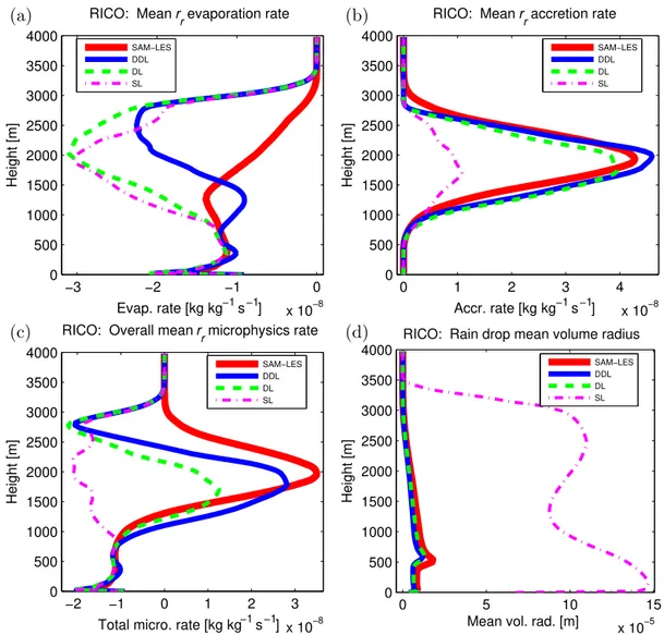
Figure 7 shows profiles of RICO mean microphysics pro-cess rates. The mean evaporation rate profile in Fig. 7a shows that all three shapes over-evaporate at higher altitudes, but that SL and DL over-evaporate more than DDL. It should be noted that the reason for the over-evaporation at higher alti-tudes in the RICO case is the marginal PDF ofχ produced by ADG2. While it provides a good match between CLUBB and SAM LES in the fields of cloud fraction andrc, the value ofσχ (1)is far too large. Whenχandrr(orNr) are distributed jointly, this results in too many large values ofrr(orNr) be-ing placed in air that is far too dry. RICO mean evaporation rate could benefit from an improved ADG2 in order to pro-duce a better marginal distribution ofχ, but that is beyond the scope of this paper.
Figure 7b shows that both the DL and DDL PDF shapes match the LES mean accretion rate profile much better than does the SL shape. The mean autoconversion rate depends onχ andNcnbut not hydrometeor variables, and so the au-toconversion rate is the same for all three PDF shapes (not shown). The overall mean microphysics rate – i.e., the sum of the evaporation, accretion, and autoconversion rates – is fit best by the DDL shape and worst by the SL shape. Both DDL and DL are a much better match to the SAM profile of rain drop mean volume radius than SL (Fig. 7d).
Figure 8 shows that all three hydrometeor PDF shapes pro-vide a good match to SAM LES for DYCOMS-II RF02. In Fig. 8d, the SL PDF shape deviates more strongly from SAM LES than does DL or DDL near the bottom of the profile of rain drop mean volume radius.
In the simulation of LBA, Morrison microphysics was used in both SAM LES and CLUBB. In order to account for subgrid variability in the microphysics, sample points from the PDF are produced at every grid level using the Sub-grid Importance Latin Hypercube Sampler (SILHS) (Raut and Larson, 2016; Larson and Schanen, 2013; Larson et al., 2005). For the LBA case, 128 sample points were drawn. Morrison microphysics is then called using each set of sam-ple points, and the results are averaged to calculate the mean microphysics process rates.
Figure 9 shows the same mean microphysics process rates as in previous figures, but here for LBA. The profile of mean evaporation rate in Fig. 9a shows that DDL is the best match to SAM LES. The profile of mean accretion rate in Fig. 9b shows that DDL is the best match to SAM, followed by DL and then SL. The overall (autoconversion+accretion+
−3 −2 −1 0
x 10−8 0
500 1000 1500 2000 2500 3000 3500 4000
RICO: Mean r
revaporation rate
Evap. rate [kg kg s ]−1 −1
Height [m]
SAM−LES DDL DL SL (a)
0 1 2 3 4
x 10−8 0
500 1000 1500 2000 2500 3000 3500 4000
RICO: Mean r
raccretion rate
Accr. rate [kg kg s ]−1 −1
Height [m]
SAM−LES DDL DL SL (b)
−2 −1 0 1 2 3
x 10−8 0
500 1000 1500 2000 2500 3000 3500 4000
RICO: Overall mean r
rmicrophysics rate
Total micro. rate [kg kg s ]−1 −1
Height [m]
SAM−LES DDL DL SL (c)
0 5 10 15
x 10−5 0
500 1000 1500 2000 2500 3000 3500 4000
RICO: Rain drop mean volume radius
Mean vol. rad. [m]
Height [m]
SAM−LES DDL DL SL (d)
Figure 7.Profiles of mean microphysics process rates in the RICO precipitating shallow cumulus case time-averaged over the last 2 hours of the simulation (minutes 4200 through 4320). The SAM LES results are red solid lines, the DDL results are blue solid lines, the DL results are green dashed lines, and the SL results are magenta dashed-dotted lines.(a)The mean evaporation rate ofrr.(b)The mean accretion rate ofrr.(c)The overall mean microphysics tendency forrr.(d)The mean volume radius of rain drops. Overall, the DDL provides a better fit to SAM LES than the DL, which in turn provides a better fit than the SL.
matched by the DDL hydrometeor PDF shape, followed by the DL shape, which in turn is followed by the SL shape (Fig. 9c).
6 Conclusions
The multivariate PDF used by CLUBB has been updated to improve the subgrid representation of hydrometeor species. The most important update is the introduction of precipita-tion fracprecipita-tion to the PDF. The precipitating fracprecipita-tion contains any non-zero values of any hydrometeor species included in the microphysics scheme. The remainder of the subgrid domain is precipitation-less and is represented by a delta function where every hydrometeor species has a value of zero. When a hydrometeor is found at a grid level, its
rep-resentation in the precipitating portion of the subgrid domain is a lognormal or double-lognormal distribution. The intro-duction of precipitation fraction increases accretion and de-creases evaporation in cumulus cases, allowing more precip-itation to reach the ground.