www.biogeosciences.net/10/1983/2013/ doi:10.5194/bg-10-1983-2013
© Author(s) 2013. CC Attribution 3.0 License.
Biogeosciences
Geoscientiic
Geoscientiic
Geoscientiic
Geoscientiic
Global ocean carbon uptake: magnitude, variability and trends
R. Wanninkhof1, G. -H. Park1,2,*, T. Takahashi3, C. Sweeney4,16, R. Feely5, Y. Nojiri6, N. Gruber7, S. C. Doney8, G. A. McKinley9, A. Lenton10, C. Le Qu´er´e11, C. Heinze12,13,14, J. Schwinger12,13, H. Graven7,15, and S. Khatiwala3
1Ocean Chemistry Division, NOAA/AOML, 4301 Rickenbacker Causeway, Miami, FL 33149, USA 2Cooperative Institute for Marine and Atmospheric Studies, University of Miami, Miami, FL 33149, USA 3Lamont-Doherty Earth Observatory of Columbia University, Route 9W, Palisades, NY 10964, USA
4NOAA/ESRL Carbon Cycle Group Aircraft Project Lead, 325 Broadway GMD/1, Boulder, CO 80304, USA 5Ocean Climate Research Division, NOAA/PMEL, 7600 Sand Point Way NE, Seattle, WA 98115, USA
6Center for Global Environmental Research National Institute for Environmental Studies Onogawa 16-2, Tsukuba, Ibaraki 305-8506, Japan
7Environmental Physics Group, Institute of Biogeochemistry and Pollutant Dynamics, ETH Zurich, 8092 Zurich, Switzerland 8Woods Hole Oceanographic Institution, Woods Hole, MA 02543, USA
9Atmospheric and Oceanic Sciences and Center for Climatic Research, University of Wisconsin – Madison, WI 53706, USA 10CSIRO Marine and Atmospheric Research, P.O. BOX 1538 Hobart Tasmania, Australia
11Tyndall Centre for Climate Change Research, University of East Anglia, Norwich Research Park, Norwich NR4 7TJ, UK 12Geophysical Institute, University of Bergen, Allegaten 70, 5007 Bergen, Norway
13Bjerknes Centre for Climate Research, Bergen, Norway 14Uni Bjerknes Centre, Uni Research, Bergen, Norway
15Scripps Institution of Oceanography, University of California San Diego, 9500 Gilman Dr., La Jolla, CA 92093, USA 16CIRES, University of Colorado, Boulder, CO 80304, USA
*now at: East Sea Research Institute, Korea Institute of Ocean Science & Technology, Uljin, 767–813, Korea
Correspondence to:R. Wanninkhof ([email protected])
Received: 30 June 2012 – Published in Biogeosciences Discuss.: 15 August 2012 Revised: 1 March 2013 – Accepted: 4 March 2013 – Published: 22 March 2013
Abstract.The globally integrated sea–air anthropogenic car-bon dioxide (CO2) flux from 1990 to 2009r is determined from models and data-based approaches as part of the Re-gional Carbon Cycle Assessment and Processes (RECCAP) project. Numerical methods include ocean inverse models, atmospheric inverse models, and ocean general circulation models with parameterized biogeochemistry (OBGCMs). The median value of different approaches shows good agree-ment in average uptake. The best estimate of anthropogenic CO2 uptake for the time period based on a compilation of approaches is−2.0 Pg C yr−1. The interannual variabil-ity in the sea–air flux is largely driven by large-scale cli-mate re-organizations and is esticli-mated at 0.2 Pg C yr−1 for the two decades with some systematic differences between approaches. The largest differences between approaches are seen in the decadal trends. The trends range from −0.13 (Pg C yr−1)decade−1to−0.50 (Pg C yr−1)decade−1for the
two decades under investigation. The OBGCMs and the data-based sea–air CO2flux estimates show appreciably smaller decadal trends than estimates based on changes in carbon in-ventory suggesting that methods capable of resolving shorter timescales are showing a slowing of the rate of ocean CO2 uptake. RECCAP model outputs for five decades show simi-lar differences in trends between approaches.
1 Introduction
comprehensive assessments of carbon flows between the ma-jor labile reservoirs, data contributions and model output are provided on volunteer basis and for a set time period (1990– 2009). Therefor not all major ocean models are represented; most notably some of the more advanced models runs for the Fifth Assessment Report (AR5) of the United Nations Inter-governmental Panel on Climate Change (IPCC) are not in-cluded. However, an appreciable number of different model outputs are used and the range of results for the different model types are representative.
The ocean exchanges CO2with the atmosphere at the sea– air interface. The exchange is driven by complex and varying physical and biogeochemical processes that make accurate assessment of the sea–air CO2flux challenging. Knowledge of the exchange is important for several processes. The mag-nitude and direction of fluxes are indicative of biogeochemi-cal cycling in the ocean. Estimates of the globally integrated sea–air fluxes are relevant for quantifying the ocean uptake of anthropogenic CO2(Sabine and Tanhua, 2010).
The anthropogenic CO2 perturbation of the ocean is caused by increasing atmospheric CO2 levels due to fos-sil fuel burning and land use changes. It is superimposed on the natural CO2 cycle. While these can be separated in models, measurements provide the combined natural and an-thropogenic component. Exchange of natural CO2 across the sea–air interface tends to dominate on regional scales (Gruber et al., 2009) but largely cancels at the global scale. The exception is the outgassing of CO2from the ocean that is driven by the input of carbon by rivers (Sarmiento and Sundquist, 1992). The global contemporary flux of CO2 is the sum of a natural CO2flux, including the river-induced outgassing flux, and the anthropogenic CO2 uptake. Both natural and anthropogenic fluxes vary with time. The anthro-pogenic CO2flux primarily responds to the increase in atmo-spheric CO2, with climate variability having a minor impact (e.g., Lovenduski et al., 2008). In contrast, the natural carbon flux is not impacted by the rise in atmospheric CO2, but can change substantially in response to climate (Le Qu´er´e et al., 2010).
Different approaches are used to estimate the ocean carbon sink. The net sea–air CO2flux across the sea–air interface provides a direct estimate of the contemporary flux. Micro-meteorological techniques such as the eddy-covariance flux method (Fairall et al., 2000) can determine the sea–air CO2 fluxes directly at local scale but with significant uncertainty, preventing a meaningful extrapolation to larger scales. At re-gional to global scale, a bulk flux expression that has a kinetic term and a thermodynamic term is used to determine sea–air CO2fluxes according to
F =k×(Cw−Ca), (1) where the kinetic term,k, is the gas transfer velocity and in-corporates all processes that control the kinetics of the gas transfer across the sea–air interface. The term (Cw–Ca)is the concentration gradient of the gas in the liquid boundary
layer that is on the order of 100 micron thick. For sea–air CO2fluxes, the equation is commonly written in terms of the partial pressure (or fugacity) difference across the interface according to
F =k×K0×(pCO2w−pCO2a)=k×K0×1pCO2 (2) where, by convention, the net flux into the ocean is expressed as negative value.pCO2w is the partial pressure of CO2 of surface water,pCO2ais the partial pressure of CO2in air,K0 is the solubility of CO2, and1pCO2 is the partial pressure gradient (1pCO2=pCO2w–pCO2a). The CO2levels in air are reported as a mixing ratio or mole fraction, XCO2a, which are converted to a partial pressure throughpCO2a=XCO2a (P–pH2O), whereP is the ambient pressure andpH2Ois the
saturation pressure of water vapor.
The principal observational approach to estimate the sea– air flux of CO2 is to make measurements of1pCO2from ships and moorings and to use a parameterization ofkas a function of wind speed. Other approaches used to infer global sea–air CO2fluxes rely on models, total dissolved inorganic carbon (DIC) measurements in the ocean interior and/or at-mospheric data. Of these methods, those relying on simula-tions with Ocean General Circulation Models with parame-terization of biogeochemical processes (OBGCMs) calculate the CO2flux using Eq. (2). In this case,pCO2wis computed from the modeled state variables of the carbonate system; total alkalinity (TAlk) and DIC. The resolution of global bio-geochemical models used in RECCAP are on the order 2 by 2◦ with output provided at monthly timescales. Ocean in-verse models constrain the regional and global fluxes from interior ocean circulation and ocean interior data based on measurements of DIC and other tracers (Mikaloff Fletcher et al., 2006, 2007; Gruber et al., 2009). The ocean inverse models provide both the natural and anthropogenic CO2 flux components on decadal scales. The inverse estimates are independent of the estimates based on1pCO2(Eq. 2). Khatiwala et al. (2009, 2012) provide estimates of changes in anthropogenic CO2 in the ocean interior using a Green function with transient tracers that yields the anthropogenic CO2uptake estimates at regional scales. Atmospheric inver-sions use atmospheric transport models and measured atmo-spheric CO2levels to assess sources and sinks of contempo-rary CO2. The faster atmospheric transport and mixing com-pared to ocean circulation leads to coarser spatial resolution but higher temporal resolution compared to ocean inversions. The atmospheric inverse models used here resolve about a dozen ocean regions (Jacobson et al., 2007). Trends in the at-mospheric ratio of O2/N2along with atmospheric CO2levels can be used to separate terrestrial CO2 uptake from that of oceanic uptake due to reservoir specific fractionation (Man-ning and Keeling, 2006; Bender et al., 2005). Scales of ocean uptake estimates from O2/N2are hemispheric and seasonal.
and air commenced in the early 1960’s but at limited scope (Fig. 1). Global physical forcing fields such as wind speeds are available for the last 5 decades, but the older estimates are not always consistent with current measurements due to large changes in observing and interpolation methods.
Here the focus is on the last 20 yr (1990–2009) with an em-phasis is on an empirical approach that utilizes the1pCO2 climatology and surface ocean temperature to estimatepCO2 variability. The global sea–air CO2 flux derived from this method is compared with models and other approaches. The background section is a summary of reported global sea–air CO2 fluxes and their uncertainties. The results of the 50 yr runs of several of the OBGCMs are used to show the vari-ability and trends in the ocean uptake. The methodology sec-tion provides an overview of how the sea–air fluxes are deter-mined for the different approaches. An empirical approach is detailed to estimate a 20 yr time series of globally inte-grated sea–air fluxes from the globalpCO2climatology, sea surface temperature (SST) and wind anomalies over the past two decades. The section also outlines the different models and other approaches used in the analysis. The discussion is focused on the anthropogenic CO2flux and details the ad-justments applied to the different modeling and observational approaches to get consistent estimates. In the last section the estimates are reconciled to provide a consistent global an-thropogenic CO2uptake. It concludes with a summary of the median anthropogenic CO2 uptake, and the subannual vari-ability (SAV) and interannual varivari-ability (IAV) of the sea–air CO2fluxes determined by the methods.
2 Background
2.1 Atmospheric CO2variability and trends
ThepCO2of air (pCO2a)is well constrained from measure-ment of the mole fraction of CO2, XCO2, in air at about 80 global flask sampling stations worldwide (Conway et al., 1994). Seasonal changes of approximately 10 ppm over the Northern Hemisphere oceans are driven by the photosynthe-sis and respiration cycle of the terrestrial biosphere. Much smaller seasonal changes are observed in the Southern Hemi-sphere due to the lack of land cover. The atmospheric CO2 measurements point towards rapid zonal atmospheric mix-ing (weeks to month) and impedance in the tropics causmix-ing slower interhemispheric exchanges on the order of a year (Denning et al., 2002). Superimposed on the natural cycle is the increase in CO2concentration from burning of fossil fuel and land use changes, the anthropogenic perturbation. The releases occur in the Northern Hemisphere with exchange of the excess CO2 to the Southern Hemisphere on annual timescales, leading to a substantial north-to-south gradient in the annual mean XCO2. Roughly half of the anthropogenic CO2 emissions accumulate in the atmosphere with the re-mainder taken up by the ocean and the terrestrial biosphere.
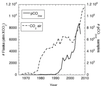
Fig. 1. Tabulation of the number of air CO2 samples (dashed
line, left axis) and surface waterpCO2 samples (solid line, right
axis) taken per year. The tabulations for air samples are from NOAA/ESRL/GMD (courtesy T. Conway, NOAA/Earth System Research Laboratory/Global Monitoring Division) and the num-bers ofpCO2surface water samples are from the SOCAT (Surface
Ocean CO2Atlas) database (Pfeil et al., 2012). Note the
hundred-fold difference in the scales of the left and right axes.
The global average increase in atmospheric CO2 concentra-tion is 1.8 ppm yr−1from 1990 to 2009.
2.2 OceanicpCO2wvariability and trends
In contrast to thepCO2over the ocean, thepCO2in the sur-face ocean (pCO2w)is spatially and temporally more vari-able, and therefore requires several orders of magnitude more data to map variations (Figs. 1 and 2). Seasonal and interan-nual changes in the surface ocean can be 100 µatm or more. The spatial decorrelation length scales are on the order of 100s of km (Li et al., 2005) compared to 1000s of km in the marine atmosphere. The greater variability and challenges in making measurements ofpCO2wmeans that for large parts of the ocean there are insufficient observations to obtain di-rect estimates of1pCO2(Fig. 2). Only select regions such as the equatorial Pacific, and time-series stations in the subtrop-ical North Atlantic (ESTOC (European Time Series in the Canary Islands) and BATS (Bermuda Atlantic Time Series)) and subtropical North Pacific (HOT (Hawaii Ocean Time-series)) have sufficient measurements and robust interpola-tion schemes to discern decadal variability and trends based on observations alone.
Fig. 2. (a)Cruise tracks with surface waterpCO2measurements.
The black lines indicate the tracks with measurements used in Taka-hashi et al. (2002) and the red lines are measurements added to the database in Takahashi et al. (2009).(b)Number of months in each 4◦by 5◦area where at least one surface waterpCO2measurement has been made since the early 1970s. White areas are pixels that have no measurements. Reproduced from Fig. 1 in Takahashi et al. (2009).
vary on multiyear timescales. The climatology is on coarse (4◦latitude×5◦longitude) resolution, and data have been in-terpolated over the annual cycle and in space using the mean surface flow fields from an OBGCM. The second approach is to interpolate the data in time and space using ancillary observations, such as SST, mixed layer depth and other sur-face parameters. No global estimate is yet available based on this approach, but regionally self-organizing maps (Tel-szewski et al., 2009) and multiparameter regressions (Schus-ter et al., 2013; Ishii et al., 2013) have been used to de(Schus-termine regional1pCO2fields and fluxes.
For variability and trends in pCO2w over the past two decades we are limited to numerical models and a scheme that utilizes the monthly pCO2 climatology of T-09 and local-scale empirical relationships of pCO2w against SST. These empirical relationships are then applied to the more comprehensive, time-varying SST record to arrive at monthly estimates (Park et al., 2010a) as detailed below.
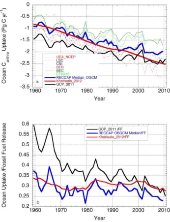
Fig. 3. (a)The 50 yr globally integrated ocean anthropogenic CO2 uptake from OBGCMs used in RECCAP. The thin solid and dashed lines show the increasing annual uptake of the different models and their interannual variability (Tables 2 and 4). The thick solid blue line is the median of the OBGCMs; the thick solid red line is the output of the Green function method (Khatiwala et al., 2012) and the thick black line is the result from the GCP ocean model ensem-ble (http://www.globalcarbonproject.org/carbonbudget/index.htm). (b)The fraction of fossil fuel taken up by the ocean over the last 50 yr. The line colors refer to the model outputs as in(a).
2.3 Factors influencing global ocean CO2uptake estimates
an appreciably greater uptake in 2010. The results from the OBGCMs suggest that while the ocean sink has increased significantly over the past 50 yr, the increase is slower than the increase in fossil fuel CO2emissions. Thus the percent of fossil fuel emissions absorbed by the oceans based on OBGCMs has steadily declined, while the Green function shows a much smaller relative decrease in uptake (Fig. 3b). The synthesis provided by the GCP shows the largest de-crease in fractional uptake. It must be noted that these 50 yr model runs lack of good information on physical forcing for the first half of the time series, which can impact the reliabil-ity of the results.
The 50 yr record of sea–air CO2 fluxes provides an im-portant benchmark but there are several shortcomings in the record, particularly as they pertain to forcing and variability. These issues are outlined below in a context of shorter and better constrained runs. The treatment of the different sea– air CO2 flux components represent a substantial challenge when comparing flux estimates. The focus here is on the an-thropogenic component of the CO2flux, which we compute from estimates of the contemporary CO2flux by subtracting the natural CO2 flux component. The latter is estimated by assuming that ocean circulation and biological activity has remained roughly constant on multidecadal scales over the last 250 yr. In this case, the natural CO2flux, when integrated over the globe, cancels to zero except for the river-carbon in-duced outgassing flux of CO2. Although this assumption pro-vides a good first estimate, the interannual variability, IAV and changes in circulation and biogeochemistry cause tem-poral fluctuations in the natural CO2flux components. More-over, there are no means of conclusively determining if the assumed centennial constancy in circulation and ocean bio-geochemistry is correct. However, the steady levels of atmo-spheric CO2in the millennia prior to the industrial revolution suggest that carbon cycling between ocean, atmosphere and terrestrial biosphere was in steady state. The deviations in natural CO2 fluxes between ocean and atmosphere are be-lieved to occur on interannual timescales and variability in the decadal averages of the natural CO2 flux component in models is less than±0.3 Pg C yr−1(Lovenduski et al., 2008). The contribution of the river-carbon induced outgassing flux to the natural sea–air flux of CO2 amounts to about +0.45 Pg C yr−1 (Jacobson et al., 2007). This needs to be accounted for when comparing model simulation of anthro-pogenic CO2uptake with contemporary flux estimates based on1pCO2measurements. The river efflux is assumed to be relatively constant through time, so that a constant offset of 0.5 Pg C yr−1is applied to the sea–air CO2fluxes based on 1pCO2to obtain the anthropogenic CO2uptake. Additional adjustments are applied to provide a uniform comparison of different estimates that include normalization of surface area of the ocean, sea ice, and coastal carbon input.
The observational benchmark for the net contemporary sea–air CO2 fluxes is the Takahashi et al. (2009) (T-09) 1pCO2 climatology. It is also the basis for our empirical
approach to estimate interannual variability. However, even with over 3 million data points and its coarse resolution, the T-09pCO2w climatology is data limited. For much of the ocean, particularly the Southern Hemisphere, the seasonal cycle cannot be fully resolved from measurements alone. As shown in Fig. 2 only in the Northern Hemisphere are there sufficient monthly observations to create a full climatologi-cal year. A propagation of errors suggests an uncertainty in the global fluxes from the climatology of 50 %. However, the calculated sea–air fluxes are in better than 50 % agreement with independent mass balance and model estimates (e.g., Gruber et al., 2009). The adjustments and breakdown of er-rors are listed in Table 1 along with an updated estimate that is described in the methods section.
The uncertainty estimates in Table 1 are described in sec-tion 6.4 of Takahashi et al. (2009). The breakdown of the uncertainty estimate shows that the smallest uncertainty in global sea–air CO2fluxes is associated with the1pCO2 es-timate. This mirrors the conclusion for a regional estimate by Watson et al. (2009) that the decorrelation length scales on the order of hundreds of kilometers and the large num-ber of measurements in each grid cell increase the certainty in1pCO2appreciably. However, the uncertainty estimate in 1pCO2 does not fully account for the dearth of measure-ments in many parts of the ocean. The uncertainty in the gas transfer velocity, k, is based on the range of common pa-rameterizations presented in the literature. Recent syntheses suggest that globally the uncertainty in gas transfer is in the range of 10 to 20 % (Ho et al., 2011), appreciably smaller than the uncertainty of 30 % in Takahashi et al. (2009). Dif-ferences in global wind products are substantial, but this is partially compensated for by normalizing gas transfer–wind speed relationships such that they match in reconstructing the global ocean bomb-14C inventories (Sweeney et al., 2007; Naegler, 2009).
The largest uncertainty in the global CO2flux climatology of T-09 is attributed to the assumption that the surface seawa-terpCO2increases at the same rate as the atmospheric CO2 levels of≈1.5 ppm yr−1for the past four decades. The uncer-tainty estimate of±0.5 Pg C yr−1is derived from assuming an uncertainty of±0.5 µatm yr−1in the oceanic CO2increase and accounting for the data distribution in time. Therefore, the assumption that the1pCO2remains invariant is critical for the climatology. For regional shorter-term assessments, where data are not normalized to a common time reference, this uncertainty does not come into play.
Table 1.Summary of different components of the globally integrated sea–air CO2flux estimate including the sources and magnitude
of the uncertainty.
Year 2000 from Takahashi et al. (2009) Updated estimatea Pg C yr−1 % Pg C yr−1 Pg C yr−1 Pg C yr−1
Net flux −1.38 −1.18
1pCO2 ±13 % ±0.18 ±0.18
k ±30 % ±0.42 ±0.2
Wind (U) ±20 % ±0.28 ±0.15
<d(pCO2w) dt−1>b ±35 % ±0.5 ±0.5
Total ±53 % ±0.7
Undersamplingc −0.2 −0.2
Riverine carbond 0.4 ±0.2 0.45 ±0.2
Coastal area −0.18
Anthro CO2flux −2.0 ±0.8e −2.0 ±0.6
For a non–El Ni˜no year 2000 (adapted from section 6, T-09).aDetails on the updated estimate are provided in the text.
bd(pCO
2w)dt−1represents the error due to uncertainty in the mean rate ofpCO2wchange of (1.5±0.2 µatm yr−1)used
for correcting observed values measured in different years to the reference year 2000.cThe bias due to spatial
undersampling is determined by using the temperature bias of 0.08◦C between the measured SST used in the T-09 climatology and a comprehensive global SST climatology. For an iso-chemical temperature dependence of 4.2 %◦C−1
forpCO2w, this translates into apCO2wbias of 1.3 µatm that in turn leads to a bias in globally integrated flux of
−0.2 Pg C yr−1. That is, the ocean sink is greater when applying this correction.dThe CO2flux from riverine carbon
input into the ocean is an efflux. To convert from the contemporary CO2flux to the anthropogenic CO2flux this value has
to be subtracted. That is, the ocean anthropogenic CO2uptake is greater than the net flux derived from the T-09
climatology.eListed as±1.0 Pg C yr−1in T-09.
Omar and Olsen, 2006; Metzl et al., 2010) show thatpCO2w has increased faster than atmospheric CO2, thereby decreas-ing the CO2 sink. In other areas such as the NW Atlantic (Park et al., 2012) and NW Pacific (Takahashi et al., 2006) pCO2w is increasing at a slower rate the atmospheric in-creases.
In the Southern Ocean, where the changes are attributed to more upwelling of deep water, the changes are believed to be sustained. Increased upwelling is attributed to increases in zonal wind stress caused by large-scale reorganizations of the Southern Hemisphere climate system in response to global warming and stratospheric ozone loss (Thompson and Solomon, 2002). In other parts of the ocean, where the changes are attributed to more ephemeral causes, no system-atic multidecadal changes in uptake are anticipated, as of yet, other than those caused by increasing atmospheric CO2 lev-els.
Winds have a major impact on sea–air CO2fluxes through their influence onk(Eq. 2). Long-term global wind records suggest an increase with time (Young et al., 2011). The global wind speed records are either based on atmospheric assimilations commonly used in weather forecasts, ship and buoy based observations, remotely sensed winds, or a com-bination thereof. Determining accurate trends is challeng-ing because of changes in procedures and inputs. Assim-ilation models (e.g., NCEP (National Center for Environ-mental Prediction), ECMWF (European Centre for Medium-Range Weather Forecasts)) are reanalyzed, often with as ma-jor objective to eliminate procedural biases. The reanaly-sis products show appreciable global and regional
differ-ences in magnitude and variability (Wallcraft et al., 2009). For the RECCAP analysis the cross-calibrated multiplatform (CCMP) winds are used as they address many of the short-comings of other products for the determination of sea–air CO2fluxes.
3 Methods
Here we provide details on the bulk flux equation (Eq. 2) in-put parameters, which are key for surface ocean data-based methods and OBGCMs that provide fluxes based on1pCO2. The updates to the input parameters used in Eq. (2) compared to T-09 are emphasized. The procedure to determine a 20 yr time record of fluxes from SST anomalies is provided. The OBGCMs, atmospheric and ocean inverse models, and esti-mates based on atmosphere O2/N2are described briefly. The model analyses used here are referred to as Tier 1 method-ologies in the RECCAP protocol (Canadell et al., 2011).
3.1 Gas transfer velocities and wind speeds
The estimate of the gas transfer velocity,k, is improved com-pared to previous assessments.
Fig. 4.Global pattern of the temporal trend of the second moment of surface wind speed< U2>for the 20 yr CCMP wind product (1990–2009). Regions where trends are at less than 90 % confidence level are masked.
observation-based estimate in RECCAP, the cross-calibrated multiplatform (CCMP) winds (Atlas et al., 2011) were cho-sen instead as the default product. The winds are pro-vided at 6 h time intervals and 0.25◦ resolution to deter-mine the mean square wind speeds, or second moments, thereby accounting in a more robust way the actual vari-ability of wind on gas transfer (Wanninkhof et al., 2009). The data are available at http://podaac.jpl.nasa.gov/DATA CATALOG/ccmpinfo.html.
The CCMP product is well documented and consistent for the entire time record. It covers the time period from 1 January 1990 to 31 December 2009, and shows apprecia-ble trends in wind speed over time both regionally and glob-ally. Figure 4 shows the decadal trends of the second moment of the winds,< U2>, used in the analyses (see Eq. 3). At 90 % significance level the trends show decreases in< U2> in the subtropical North Pacific and increases in the South-ern Ocean and equatorial Pacific. The increasing winds have a direct effect on the sea–air CO2flux through an impact on the gas transfer velocity but also an indirect effect on1pCO2 from the wind impact on ocean circulation and mixed layer dynamics.
A procedure similar to Wanninkhof (1992) is used to deter-mine the gas transfer–wind speed relationship. The gas trans-fer velocity is modeled as having a quadratic dependency with wind based on extensive wind tunnel and field studies. The magnitudes of gas transfer velocities determined from the second moments of the CCMP wind product are used in an inverse procedure to solve for the inventory of bomb14C in the ocean (Sweeney et al., 2007). The procedure optimizes for the coefficient of the gas transfer velocity,a:
a=k < U2>−1, (3) wherekis the gas transfer velocity (cm h−1), “< >” denote temporal averages, and< U2>(m s−1)2is the time mean of the second moment of the wind speed at 10 m height. The coefficient,a((cm h−1)(m s−1)−2), is adjusted such that the bomb-14C inventory increase in the ocean corresponds with
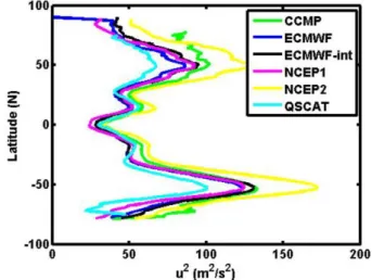
Fig. 5. Comparison of the zonal mean distribution of the second moment of ocean surface winds for the year 2000 for several global wind products. Differences of up to 30 m2s−2(wind speed differ-ence≈4 m s−1) are observed, and the biases are not always con-sistent between high and low latitudes. CCMP=Cross Calibrated Multi-Platform winds (Atlas et al., 2011); ECWMF= European Center for Medium Weather Forecasting; NCEP=National Center for Environmental Prediction; QSCAT=QuikSCAT polar orbiting satellite with an 1800 km wide measurement swath on the earth’s surface equipped with the microwave scatterometer SeaWinds.
the atmospheric 14C history. In Sweeney et al. (2007) the NCEP-II winds were used to optimizeawhile here the opti-mization was rerun for the CCMP winds thereby decreasing the uncertainty and bias in the flux using the CCMP wind product.
The optimal coefficient for the gas transfer velocity parame-terization is 0.251 and:
3.2 The impact of the updated gas transfer velocity parameterization on global fluxes
The CCMP wind product averaged over the 4◦×5◦ grid yields a global average, 20 yr mean, wind speed <U> of 7.6 m s−1 and a second moment, < U2> of 69.1 (m s−1)2. Equation (4) yields a global average gas transfer velocity<k> of 15.95 cm h−1, and a global sea–air CO2 flux of −1.18 Pg C yr−1 when applied to the Takahashi 1pCO2 climatology (downloaded Octo-ber 2010 from: http://www.ldeo.columbia.edu/res/pi/CO2/ carbondioxide/pages/air sea flux 2010.html). For compari-son the net sea–air flux determined by T-09 using NCEP-II winds is−1.38 Pg C yr−1(Table 1). The 15 % difference in-dicates the sensitivity of global sea–air fluxes to wind speed product and wind speed parameterization.
3.3 Method for estimating interannual variability (IAV) and decadal trends in 1pCO2 using a data-based approach
There are limited observational data on global trends and variability in ocean sea–air CO2 fluxes. An empirical ap-proach first presented in Lee et al. (1998) and improved in Park et al. (2010a), henceforth referred to as P-10, pro-vides an assessment of IAV based on seasonal correlations of pCO2w and SST that are used with the measured in-terannual SST variability. This approach is applied to the T-09 climatology as follows: The monthly mean sea–air CO2 flux for each 4◦×5◦ grid cell for an individual year other than the climatological year 2000 is estimated from the global pCO2w climatology, andpCO2w anomalies de-termined from subannualpCO2w–SST relationships. Suban-nual timescales are defined as seasonal to up to a year. The subannualpCO2w–SST relationships are derived from one to four linear fits ofpCO2w and SST for each of the 1759 4◦×5◦ grid cells in the T-09 climatology. The number of subannual segments chosen to delineate the subannual trends is kept to a minimum but sufficient to characterize the rela-tionship betweenpCO2w and SST for each location. Fewer unique segments decrease the uncertainty in the pCO2w– SST relationships. The monthly< U2>is from the CCMP product, and the monthly mean SST is from the NOAA Optimum Interpolation (OI) SST product (Reynolds et al., 2007; http://www.cdc.noaa.gov/data/gridded/data.noaa.oisst. v2.html). Sea level pressures from NCEP-II for each grid cell are used to determine thepCO2afrom the measured XCO2a. Details are provided in Park et al. (2010b).
For the central and eastern equatorial Pacific (6◦N–10◦S and 80◦W–165◦E) empiricalpCO2w–SST equations are de-rived from a large quantity of multiyear observations that were collected from 1979 to 2008 (updated from Feely et al., 2006). Based on the observations over the last several decades it is clear that the drivers of IAV in this region are different from those of seasonal variability (Ishii et al., 2013).
The period of investigation covers seven El Ni˜no and five La Nina periods. UniquepCO2w–SST equations for three dif-ferent time periods (1979–1989, 1990–1998, and mid-1998– 2008) that reflect the modulation of ENSO (El Ni˜no/Southern Oscillation) by the Pacific Decadal Oscillation (PDO) are used. Using these relationships, the IAV based on the annual values for this region is 0.07 Pg C yr−1 (1σ) for the 1990– 2009 time period.
The empirical method of P-10 to assess IAV is tied to the 1pCO2 climatology referenced to year 2000. Changes in biogeochemistry of surface seawater associated with SST changes will be reflected as long as the same mechanisms that relate subannualpCO2wchange to SST control the inter-annualpCO2w–SST relationships. A weak increasing trend inpCO2w, associated with surface ocean warming is esti-mated by the P-10 method over the 20-year period. This leads to a reduction in net global ocean CO2uptake (see below).
The P-10 method implicitly assumes thatpCO2wincreases at the same rate as atmospheric CO2 levels, that is, the 1pCO2 remains constant on multiyear scales. It thus can-not reproduce trends tied to increasing atmospheric CO2 level. To account for varying regional interannual changes in 1pCO2the “CO2-only” run of NCAR CCSM-3 model (Na-tional Center for Atmospheric Research’s Community Cli-mate System Model Version 3; Doney et al., 2009a, b) for the period of 1987–2006 is used. This model output is pro-duced using a repeat annual cycle of physical forcing and rising atmospheric CO2. In each 4◦×5◦grid cell, the trend in modeledpCO2wis computed by a linear regression with deseasonalized monthly values using a harmonic function. Approximately 75 % of the grid cells have statistically signif-icant positive or negative trends in1pCO2(p <0.05) over the past two decades. For the remaining 25 % of the grid cells with no significant trends in1pCO2, thepCO2w increases at the same rate as atmospheric CO2. From these trends the “CO2-only” fluxes are determined for each grid cell and they are added to CO2 fluxes from the empirical model to esti-mate the total contemporary sea–air CO2flux from 1990 to 2009. Global maps of the trends of the CO2-only output, us-ing a different model but with similar results, can be found in Fig. 4b of Le Qu´er´e et al. (2010).
3.4 Ocean global circulation models with biogeochemistry (OBGCMs)
de l’Environnement) and UEA (University of East Anglia) models include the input of riverine carbon but the input does not contribute to subsequent outgassing. Therefore, the flux estimates from all models provide the contemporary sea–air CO2flux. However, since without riverine carbon outgassing the natural CO2flux component is globally nearly balanced (≈0), the contemporary flux in the OBGCMs used equals the sea–air anthropogenic CO2flux.
3.5 Other methods of determining global sea–air CO2fluxes
Several other global estimates that rely on changes in atmo-spheric or oceanic anthropogenic CO2inventories are com-pared. These include results from eleven atmospheric inverse models provided by RECCAP, those relying on the atmo-spheric O2/N2 record, and ocean inventory changes using transient tracers based on a Green function analysis. Atmo-spheric inversions rely on the interpretation of atmoAtmo-spheric CO2gradients, but given the under-constrained nature of this inversion, they need prior information for the sea–air CO2 fluxes. Sea–air CO2 flux climatologies such as that of T-09 are used as priors. As a result, these estimates are contem-porary fluxes and include natural (with river outgassing) and anthropogenic CO2fluxes. As they use the observed sea–air CO2flux as a prior they are not a truly independent estimate of sea–air CO2 fluxes. In contrast, the atmospheric O2/N2 approach provides a strong independent constraint for the anthropogenic CO2 flux component only. Estimates based on O2/N2trends in the atmosphere from 1989–2003 can be found in Manning and Keeling (2006), while results from 2000–2010 are presented in Ishidoya et al. (2012).
The anthropogenic CO2 uptake inferred from chang-ing oceanic inventories is further detailed in Khatiwala et al. (2012). Briefly, the inventory-based estimates include an empirical Green function approach (Khatiwala et al., 2009, 2012) and ocean inversion model-based approaches, which are synthesized in the ocean inversion project (OIP) (Mikaloff Fletcher et al., 2006; Gruber et al., 2009). These approaches are based on the assumption of a steady-state ocean circulation and biogeochemistry and, therefore, only resolve the smoothly evolving changes in the oceanic uptake of anthropogenic CO2driven by the increase in atmospheric CO2. That is, they do not resolve interannual and subannual variability.
4 Discussion
4.1 Global sea–air CO2fluxes
A tabular summary of the decadal mean anthropogenic CO2 uptake centered on the year 2000, based on observations and the median value of different types of models, is provided in Table 3. The IAV, SAV and trends of the contemporary sea– air CO2flux are shown in Table 3 as well. The IAV and SAV
are dominated by the natural CO2flux. The trend from 1990– 2009 is primarily caused by the anthropogenic component with modulation by the natural cycle.
The empirical estimates of sea–air fluxes follow the pro-cedures and assumptions of T-09 and P-10 with the adapta-tions described in Sect. 3. The fluxes are extrapolated to in-clude the coastal regions by scaling to the increased surface area assuming that the fluxes in the coastal regions are the same as for the adjacent region used in the OIP. Fluxes in the coastal area are highly variable but net fluxes on the whole appear similar to that of adjacent ocean areas, with some re-gional exceptions. Eastern upwelling zones show large ef-fluxes near the coast, and riverine dominated shelves show influxes (Borges et al., 2005; Chavez et al., 2007; Liu et al., 2010; Cai, 2011). Incorporating the coastal fluxes based solely on area increases the influx by −0.18 Pg C yr−1. A global synthesis of ocean-margin carbon uptake estimates a flux of−0.29 Pg C yr−1 (Jahnke, 2010), but the shelf area in this estimate is twice that of the areal adjustment applied here.
The differences in assumptions compared to those used in T-09 lead to a 0.19 Pg C yr−1 smaller open ocean contem-porary CO2uptake (Table 1). Several adjustments are made to the contemporary flux to obtain a global anthropogenic flux. These adjustments yield an anthropogenic CO2flux of −2.0 Pg C yr−1 that is the same as the −2.0 Pg C yr−1 es-timate presented in T-09. As shown in Table 1, the lower contemporary uptake in the open ocean is compensated for by including the influx in coastal areas of −0.18 Pg C yr−1 in our flux determination. Our estimate has an uncertainty of 0.6 Pg C yr−1compared to 0.8 Pg C yr−1in T-09. This is largely due the reduced uncertainty in the determination of gas transfer velocities and winds.
Models and atmospheric observing approaches generally report smaller uncertainties than those based on surface CO2 levels and bulk flux approaches. The uncertainties in models are determined in a different fashion and generally expressed in terms of a deviation from multimodel ensemble compar-isons. An important consideration when determining uncer-tainty in this fashion is that model architecture and forcing are often similar, which can lead to an unrealistic good cor-respondence between them. Graphical summaries of the sea– air anthropogenic CO2fluxes for the OBGCMs and ocean in-verse estimates, and the atmospheric inversions from 1990 to 2009 are presented in Figs. 6 and 7, respectively. A summary of the medians of different methods is shown in Fig. 8.
Table 2.Ocean general circulation models with biogeochemistry (OBGCMs)a.
Abbreviation Name Key Reference Years used
BER MICOM-HAMOCCv1 Assmann et al. (2010) 1990 to 2009 CSI CSIRO-BOBGCM Matear and Lenton (2008) 1990 to 2009 BEC CCSM-BEC Doney et al. (2009a, b) 1990 to 2009 ETHbk15 CCSM-ETHk15 Graven et al. (2012) 1990 to 2007
ETHck19 CCSM-ETHk19 – 1990 to 2007
LSC NEMO-PISCES Aumont and Bopp (2006) 1990 to 2009 UEAdNCEP NEMO-PlankTOM5NCEP Buitenhuis et al. (2010) 1990 to 2009
UEAeECMWF NEMO-PlankTOM5ECMWF – 1990 to 2009
UEAfCCMP NEMO-PlankTOM5CCMP – 1990 to 2009
aFurther details on models are provided in the key reference and the RECCAP website:
http://www.globalcarbonproject.org/reccap/products.htm.bETHk15: CCSM-ETH model with a prescribed global average
gas transfer velocity of 15 cm h−1.cETHk19: CCSM-ETH model with a prescribed global average gas transfer velocity
of 19 cm h−1.dUEANCEP: NEMO-PlankTOM5 model with NCEP core forcing.eUEAECMWF: NEMO-PlankTOM5
model with NCEP core forcing but using ECWMF winds.fUEA
CCMP: NEMO-PlankTOM5 model with NCEP core
forcing but using CCMP winds.
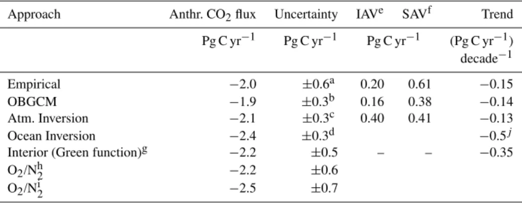
Table 3.Median sea–air anthropogenic CO2fluxes for the different approaches centered on year 2000.
Approach Anthr. CO2flux Uncertainty IAVe SAVf Trend
Pg C yr−1 Pg C yr−1 Pg C yr−1 (Pg C yr−1) decade−1
Empirical −2.0 ±0.6a 0.20 0.61 −0.15 OBGCM −1.9 ±0.3b 0.16 0.38 −0.14 Atm. Inversion −2.1 ±0.3c 0.40 0.41 −0.13 Ocean Inversion −2.4 ±0.3d −0.5j Interior (Green function)g −2.2 ±0.5 – – −0.35
O2/Nh2 −2.2 ±0.6
O2/Ni2 −2.5 ±0.7
aRoot mean square of uncertainty in different components of the flux (see Table 1).bMedian absolute deviation of the six
model outputs used to determine the median (for 6 model outputs: LSC, UEANCEP, CSI, BER, BEC and ETHk15).c
Median absolute deviation of eleven model outputs used to determine the median.dMedian absolute deviation of the ten model outputs used to determine the median.eInterannual variability (IAV) for the median values for the 6 models listed in
b.fSubannual variability (SAV) for the median values (for 5 model outputs: LSC, UEA
NCEP, CSI, BEC and ETHk15).g
Based on interior ocean changes using transient tracers and a Green function (Khatiwala et al., 2009, 2012).hFor 1993–2003 (Manning and Keeling, 2006).iFor 2000–2010 (Ishidoya et al., 2012).jCalculated assuming steady ocean circulation and CO2uptake proportional to atmospheric CO2increases.
in ocean inversions include the partitioning of anthropogenic from natural dissolved inorganic carbon. The largest un-certainty lies in ocean transport and mixing. The average anthropogenic CO2 uptake by the inversions provided in RECCAP is an update of the OIP (Mikaloff Fletcher et al., 2006; Gruber et al., 2009) with results shown in Fig. 6. The reported values for 1994 were scaled by a factor of 1.109 and 1.23 for the years 2000 and 2005, respectively, based on the scaling used in the inversion procedure itself (Mikaloff Fletcher et al., 2006). The globally integrated sea– air anthropogenic CO2 fluxes, nominally, for 1995, 2000 and 2005 are−2.18±0.25,−2.42±0.28, and−2.68±0.31 (1σ )Pg C yr−1, respectively.
Jacobson et al. (2007) present a comprehensive joint ocean–atmosphere inversion scheme applying both
atmo-spheric inverse and oceanic inverse constraints that in-clude sea–air CO2 flux estimates modified from Takahashi et al. (2002). The resulting contemporary sea–air fluxes are heavily weighted towards the (interior) oceanic in-verse due to the large number of interior data points and sluggish ocean circulation/transport compared to the at-mosphere. It yields results of an anthropogenic flux of −2.1 Pg C yr−1for the time period from 1992–1996 with an uncertainty of±0.2 Pg C yr−1, which is similar to the value of−2.18 Pg C yr−1of Gruber et al. (2009). The uncertainty is lower than that of Gruber et al. (2009) primarily because Jacobson et al. (2007) use a smaller number of general circu-lation models in their analyses.
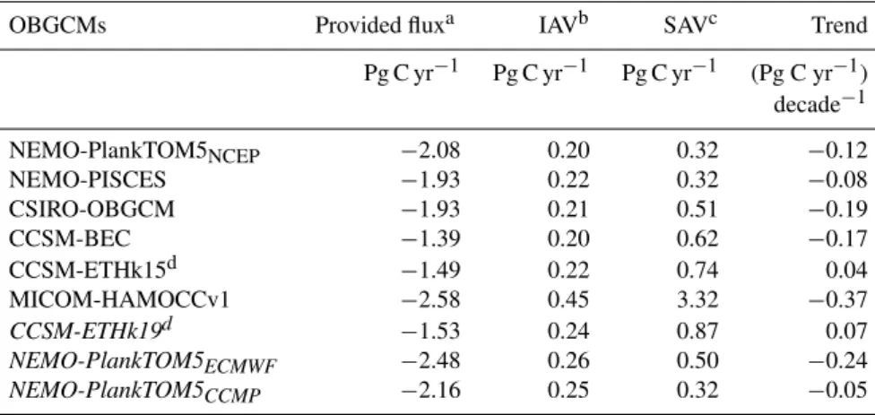
Table 4.Comparison of sea–air anthropogenic CO2flux, interannual and subannual variability of individual OBGCM outputs used.
OBGCMs Provided fluxa IAVb SAVc Trend
Pg C yr−1 Pg C yr−1 Pg C yr−1 (Pg C yr−1) decade−1
NEMO-PlankTOM5NCEP −2.08 0.20 0.32 −0.12
NEMO-PISCES −1.93 0.22 0.32 −0.08 CSIRO-OBGCM −1.93 0.21 0.51 −0.19
CCSM-BEC −1.39 0.20 0.62 −0.17
CCSM-ETHk15d −1.49 0.22 0.74 0.04 MICOM-HAMOCCv1 −2.58 0.45 3.32 −0.37
CCSM-ETHk19d −1.53 0.24 0.87 0.07
NEMO-PlankTOM5ECMWF −2.48 0.26 0.50 −0.24 NEMO-PlankTOM5CCMP −2.16 0.25 0.32 −0.05
aThis analysis is performed without the adjustment to a common ocean surface area (Supplement A).bIAV of median
values: 0.16 (for 6 models: LSC, UEANCEP, CSI, BER, BEC and ETHk15). The italicized models are excluded from
the calculation of IAV and SAV in Table 3.cSAV of median values: 0.38 (for 5 models: LSC, UEANCEP, CSI, BEC
and ETHk15). In addition to the italicized models, the MICOM-HAMOCCv1 is excluded from the summary of
OBGCMs in Table 3 as it shows extremely high SAV due to known model deficiencies.dFor the period of 1990–2007.
Fig. 6. The 20 yr record of annual globally integrated sea–air CO2fluxes from the ocean general circulation models, OBGCMs
(dashed lines), and ocean inversion estimates (circles with uncer-tainty bars). Similar line types for the OBGCMs indicate that the models have the same heritage. The median (solid red line) is the median of UEANCEP, LSC, CSI, BER, BEC and ETHk15 model
outputs.
at higher temporal resolution rely on ocean general circu-lation models with biogeochemistry (OBGCMs). A compre-hensive synthesis of model performance on a previous gener-ation OBGCMs was provided as part of the OCMIP (Ocean Carbon-Cycle Model Intercomparison Project) in the early 2000s (see e.g., Doney et al., 2004; Matsumoto et al., 2004). A more recent subset of models was used to determine the ocean sink for 1959–2008 (Le Qu´er´e et al., 2009; Sarmiento et al., 2010). Initialization, forcing and biological represen-tation for the model output used here differ for the models as summarized in the metadata on the RECCAP website and references in Table 2. The models were run in hindcast mode,
Fig. 7.The 20 yr record of annual globally integrated sea–air CO2
fluxes from atmospheric inverse models. The red line is the median of all the inverse models shown.
i.e., they were driven by atmospheric forcing assimilation products such as NCEP or ECWMF, and with a prescribed atmospheric CO2concentration using an observation based product such as GLOBALVIEW-CO2(2011).
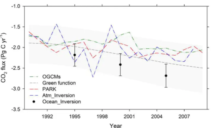
Fig. 8.The 20 yr record of annual globally integrated sea–air CO2 fluxes for the different modeling approaches. For the OBGCMs and atmospheric inverses, the lines are plotted through the annual me-dian values.
in ocean uptake due to reduced outgassing of CO2 in the equatorial Pacific (Feely et al., 2006). The models show greatly varying responses in phasing, magnitude and dura-tion of CO2flux anomalies (Fig. 6). The CCSM models show a peak-to-peak change of 0.2 Pg C yr−1, while the NEMO (Nucleus for European Models of the Ocean) models show peak-to-peak changes of up to 1.0 Pg C yr−1. The MICOM-HAMOCCv1 (Miami Isopycnic Coordinate Ocean Model-Hamburg Ocean Carbon Cycle version 1) model shows no global response to the El Ni˜no, while the CSIRO (Com-monwealth Scientific and Industrial Research Organisation) shows an increase in uptake over several years. The P-10 record shows an anomaly of about 0.3 Pg C yr−1with a re-covery in less than 2 yr (Figs. 8 and 10d).
For the estimate of the median anthropogenic CO2 up-take of the OBGCMs, we excluded model outputs that were largely similar and only differed in their forcing and, there-for, showed very similar results (Fig. 6). That is, only one of the three UEA model outputs (UEANCEP) and one of the two ETH (Swiss Federal Institute of Technology Zurich) (ETHk15)model outputs were used. The solid red line in Fig. 6 is the annual median of LSC, UEANCEP, CSI, BER, BEC and ETHk15 runs. The IAV of the median estimate of 0.16 (1σ )Pg C yr−1is damped compared to the mean IAV of the individual models of 0.25 (1σ )Pg C yr−1, indicating that the variability in the individual models is not coherent. The median trend in anthropogenic CO2uptake of the 6 models is−0.14±0.02 Pg C yr−1decade−1(p <0.01). The median trend agrees with the trends of the individual models, that span the entire time period, indicating that each behaves sim-ilarly to the increase in atmospheric CO2.
Ocean anthropogenic CO2uptake determined from atmo-spheric inverse models has a median value of−2.1 Pg C yr−1 (Table 3). The range and median of the uptake is simi-lar to that of the OBGCMs (Fig. 8). The flux for atmo-spheric inverse models is 0.3 Pg C yr−1less than that of the
ocean inversion model. The IAV is considerably greater at 0.40 Pg C yr−1(1σ ), based on the detrended median values of deseasonalized monthly anomalies (Table 3).
As with the OBGCMs, the response of the fluxes from the atmospheric inversions to the 1998 El Ni˜no varies appre-ciably from no impact to about 1.0 Pg C yr−1. However, the atmospheric inversions that give a response show the max-imum ocean uptake a year earlier (1997). The atmospheric inversions separate the seasonal and interannual CO2flux of the ocean from that of the terrestrial biosphere that shows subannual variability in CO2 exchange that is an order of magnitude greater. Therefore, the uncertainty of the separa-tion between ocean and terrestrial carbon fluxes dictates the variability in the adjacent oceans. The time-averaged glob-ally integrated anthropogenic CO2flux into the oceans from the atmospheric inversions is not independent from data-based estimates since the1pCO2fields used in the CO2flux climatology are used as a prior within the inversion. No es-timate of the decadal trend is provided, as the atmospheric inversion runs from which the median estimate is determined differ in time span and time period.
4.2 Trends and variability in wind,1pCO2and fluxes
The trends and variability in fluxes as determined from the bulk flux equation (Eq. 2) are driven by changes in wind and 1pCO2. They are discussed in the context of the empirical approach in P-10. The impact of changing winds is different than that of OBGCMs as OBGCMs are dynamic in nature and higher winds in models will not only change the rate of gas exchange, but also the1pCO2field. For instance, higher winds in OBGCMs can result in decreased net flux into the ocean through enhanced upwelling of remineralized CO2(Le Qu´er´e et al., 2007; Lovenduski et al., 2008). In contrast, ap-plying higher winds to a static1pCO2field such as the T-09 climatology will result in increased CO2uptake.
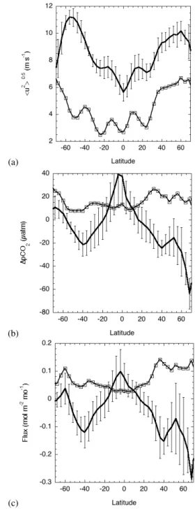
At latitudes greater than 60◦wind speeds decrease slightly. The variance pattern of winds, expressed as the standard de-viation from the 20 yr mean in Figure 9a, differs between the northern and southern hemisphere. There is more variability in winds in the mid- to high-latitudes (>30◦) in the Northern Hemisphere than in the Southern Hemisphere. Variability is at a minimum in the high-pressure regimes in the subtropics, and at the equator.
The annual mean 1pCO2 from the T-09 climatology (Fig. 9b) shows maximum values just south of the equator and a decline to the north and south. The1pCO2equals ap-proximately 0 near 18–20◦and reaches a minimum of−20 to−25 µ atm at 40◦for both hemispheres. At high northern latitudes the average1pCO2continues to drop precipitously while in the Southern Hemisphere it increases and, on clima-tological annual average, becomes slightly positive near the Antarctic ice edge causing a net CO2flux to the atmosphere (Lenton et al., 2013). The variance in1pCO2in the North-ern Hemisphere is appreciably greater than in the SouthNorth-ern Hemisphere, as is the case with the wind speed.
The flux density, computed from a 20 yr wind speed record and the climatologicalpCO2, mirrors the trends in1pCO2 but with amplification at mid-latitudes due to higher winds. The largest sink per unit area is in the Northern Hemi-sphere, but the substantially larger surface area in the South-ern Hemisphere causes a much greater spatially integrated mass exchange (see Table 6 in T-09). Because the variance in wind speed and1pCO2 have the same pattern, the flux density at mid- to high-latitudes in the Northern Hemisphere show twice the SAV compared to the Southern Hemisphere.
The greater SAV in CO2flux in the Northern Hemisphere compared to the Southern Hemisphere is likely because of the significantly greater landmasses in the north. The land– ocean contrast, along with continental input and bathymetry, causes greater variability in weather systems, (micro) nutri-ent input and seasonal temperature variations in the North, all which contribute to higher variability in sea–air CO2flux density.
Supplement B (Fig. B1b) shows a global map of SAV. Re-gions with high variability include the upwelling region in the Arabian Sea caused by the high winds in the summer monsoon. High variability from the annual mean of the sea– air CO2fluxes are also found in the eastern tropical South Pa-cific, attributed to variations in upwelling along the western boundary. In the southwestern Atlantic, near the Malvinas confluence area, SAV in fluxes is caused by variation in cur-rents, shallow bathymetry and associated plankton blooms. Low SAV is seen in the subtropical and subpolar region of the southeast Pacific and eastern tropical and subtropical South Pacific.
The patterns of SAV differ from the interannual variability (IAV) for parts of the oceans as shown in Supplement B (see Figs. B1b and B2b, respectively). There is high SAV and IAV in the North Atlantic. The equatorial Pacific shows relatively small SAV but large IAV caused by the ENSO, which
op-(a)
(b)
(c)
Fig. 9.Latitudinal distribution of zonal means (thick solid line) and standard deviations (spatial and temporal variability; thin solid line with squares) for the:(a)square root of the second moment
< U2>0.5 of the 20 yr monthly mean CCMP wind product;(b)
1pCO2from the monthly Takahashi et al. (2009) climatology; and (c)the specific sea–air CO2flux [mol m2month−1] computed by
applying the 20 yr CCMP wind product to the TakahashipCO2
cli-matology using Eq. (2). The error bars on the zonal means indicate the spatial variability (standard deviation) of means for the 5◦ lon-gitude bins in the particular latitude band.
indicating that variability on seasonal timescales dominates (Fig. B3). In the equatorial and high latitude areas the ra-tio is greater than 0.4 and in places the rara-tio is greater than 1.0, indicating that IAV exceeds subannual changes. The re-gions with high IAV correspond with those strongly affected by climate reorganizations: the North Atlantic Oscillation (NAO) in the North Atlantic; the El Ni˜no/Southern Oscil-lation (ENSO) in the equatorial Pacific and equatorial Indian Ocean; and the Southern Annual Mode (SAM) in the South-ern Ocean.
The time span of this study of two decades is at the lower limit to quantify decadal trends. On first order, pCO2w is expected to track atmospheric pCO2a increases on longer timescales. The surface ocean is closely coupled with the lower atmosphere through rapid sea–air gas exchange and relatively slower exchange between the surface mixed layer and waters below. Longer-term secular trends in1pCO2can arise from changes in circulation and upwelling patterns, and associated changes in biological productivity. The trends are also impacted by the rapid rise in atmospheric CO2, finite uptake capacity of the surface mixed layer, and decreasing buffer capacity. In absolute sense, the amount of fossil fuel derived CO2taken up by the ocean increases (Figs. 3a and 8). In a fractional sense, these factors can lead to a diminished uptake of anthropogenic CO2(Fig. 3b).
The trend in the global annual flux for the empirical ap-proach, not accounting for atmospheric CO2 increase, is 0.07±0.06 (Pg C yr−1)decade−1 over the last two decades (Fig. 10d). This decreasing uptake, in the absence of an at-mospheric CO2increase, suggests a strengthening of ocean CO2 sources or weakening of CO2 sinks, due to changes of 1pCO2 or wind speed. The second moment of the wind speed increases by 0.32±0.04 (m s−1)2 per year, which translates into about a 0.2 m s−1 increase per decade (Fig. 10a). Global SST as determined from the NOAA OI SST product (Reynolds et al., 2007) shows an increas-ing trend of 0.08±0.03 (◦C yr−1)decade−1(Fig. 10b). The trends in SST impact the1pCO2and wind will impact gas transfer in the P-10 approach. An analysis holding either the SST or wind constant in the P-10 approach indicates that the changes in the wind and SST can act synergistically or antag-onistically on the trend in fluxes depending on the region. For example, at high northern latitudes the trends in winds and SST cause an increasing CO2sink over the past two decades; in the equatorial Pacific the impact of winds and SST cause a larger CO2source; while in the Southern Ocean, the change in1pCO2due to changing SST will decrease the sink while the winds work in an opposing fashion.
The global trends in sea–air CO2flux from 1990–2009 are strongly influenced by significant IAV in1pCO2(Fig. 10c). In particular, the large El Ni˜nos in 1992/93 and 1998 de-creased the equatorial 1pCO2 and, thus, have the net ef-fect of increasing the globally integrated CO2 flux into the ocean (Fig. 10d). The changes in flux by these events are large enough to impact the trend over the 2 decades. Thus,
Fig. 10.20 yr global ocean trends in:(a)second moment of wind speed; (b) SST; (c) 1pCO2, assuming no atmospheric CO2
in-crease (gray line) and including atmospheric CO2 forcing (black
line); and(d)globally integrated contemporary sea–air CO2flux
over the past two decades (1990–2009) without atmospheric CO2
forcing (gray line) and including atmospheric CO2forcing (black
line). The change in1pCO2is determined according to the pro-cedures of Park et al. (2010a). The slopes for the linear regres-sions (solid line) for area-weighted< U2>, SST,1pCO2and flux are 0.32±0.04 (m s−1)2yr−1; 0.08±0.03 (◦C yr−1)decade−1;
−0.3±0.3 (µatm yr−1)decade−1including atmospheric CO2
forc-ing; and−0.15±0.06 (Pg C yr−1)decade−1including atmospheric CO2forcing, respectively.
climate reorganizations on multiannual timescales have an appreciable impact on the trends over the 2 decades.
4.3 Summary of global sea–air anthropogenic CO2 fluxes and trends in models
caused by more mundane issues that have been corrected for, such as estimates of global ocean surface area and conver-sion of areal representations, and different representations of sea ice. This is shown in Supplement A, where the outputs of the OBGCMs are normalized for area by determining the average flux in each of the 23 surface regions of the ocean inversion and then integrating over the area of each of the re-gions as provided in RECCAP; leading to adjustments up to 0.3 Pg C and better agreement between model runs.
Most models show trends of increasing anthropogenic CO2 uptake from 1990 to 2009 (or 2007). The median for the empirical approach, OBGCMs, and atmospheric inver-sions all show a consistent change in the anthropogenic CO2 uptake of −0.13 to −0.15 (Pg C yr−1)decade−1 over the time period, which is the same as that inferred from the approach in P-10 when including the atmospheric CO2 in-creases. Khatiwala et al. (2009; 2012) estimate an increase of inventory change of−0.35 (Pg C yr−1)decade−1based on inventory changes in anthropogenic CO2using a Green func-tion formulated from transient tracers. By construcfunc-tion, the Green function approach uptake is smooth, monotonic over time, and proportional to the atmospheric CO2increase.
5 Conclusions
An update of the sea–air CO2flux based on the1pCO2 cli-matology of Takahashi et al. (2009) (T-09), and the average 20 yr CCMP wind product, yields an anthropogenic CO2flux of -2.0 Pg C yr−1 with an uncertainty of 0.6 Pg C yr−1. This estimate includes adjustments for undersampling, coastal ar-eas and riverine inputs. Using an empirical approach relating 1pCO2to SST changes according to Park et al. (2010a) (P-10) together with model output including the effect of in-creasing atmospheric CO2 levels suggests a decadal trend of −0.15 (Pg C yr−1)decade−1. The trend indicates that the ocean sink was increasing over the past two decades. The results of this empirical approach are in good agree-ment with median anthropogenic CO2 uptake for 2000 and decadal trends for 6 OBGCMs of−1.9 Pg C yr−1and−0.14 (Pg C yr−1) decade−1, and the median 12 atmospheric in-versions of−2.1 Pg C yr−1and−0.13 (Pg C yr−1)decade−1. The anthropogenic CO2 uptake based on interior measure-ments shows a greater anthropogenic CO2uptake, but within the uncertainty of other measurements. However, trends based on ocean interior carbon changes or tracer methods are significantly greater. The transient tracer based Green function approach of Khatiwala et al. (2009, 2012) yields an anthropogenic CO2uptake of−2.2 Pg C yr−1and a decadal trend of−0.35 (Pg C yr−1)decade−1. Ocean inversions show an uptake for 2000 of−2.4 Pg C yr−1and a prescribed trend of −0.5 (Pg C yr−1)decade−1. As the ocean interior esti-mates reflect changes over longer timescales, the difference in trends for the different methods could be caused by the decreasing efficiency in ocean uptake with time. However,
the trends for the P-10 method and OBGCMs over the two decades are influenced by IAV in sources and sinks, which do not show up in the ocean interior estimates.
Supplementary material related to this article is available online at: http://www.biogeosciences.net/10/ 1983/2013/bg-10-1983-2013-supplement.pdf.
Acknowledgements. We wish to thank Joaquin Tri˜nanes for processing the CCMP wind data. RW, G-HP., RAF were sup-ported in part through the Global Carbon Data Management and Synthesis Project of the NOAA Climate Program Office. NG and HG were supported by funds from ETH Zurich and through the FP7 projects CarboChange (Project reference 264879) and GeoCarbon. CS was supported by grants, NSF/OPP 0944761 and NOAA NA12OAR4310058. SCD acknowledges support through the NOAA Climate Process Team activity, NOAA grant NA07OAR4310098. CH and JS were supported through EU FP7 project COMBINE (grant agreement no. 226520), the Research Council of Norway funded project CarboSeason (185105/S30), the Norwegian Metacenter for Computational Science and Storage Infrastructure (NOTUR and Norstore, “Biogeochemical Earth system modeling” projects nn2980k and ns2980k) and the core project BIOFEEDBACK of the Centre for Climate Dynamics (SKD) within the Bjerknes Centre for Climate Research.
Edited by: C. Sabine
References
Andres, R. J., Boden, T. A., Br´eon, F.-M., Ciais, P., Davis, S., Erick-son, D., Gregg, J. S., JacobErick-son, A., Marland, G., Miller, J., Oda, T., Olivier, J. G. J., Raupach, M. R., Rayner, P., and Treanton, K.: A synthesis of carbon dioxide emissions from fossil-fuel com-bustion, Biogeosciences, 9, 1845–1871, doi:10.5194/bg-9-1845-2012, 2012.
Assmann, K. M., Bentsen, M., Segschneider, J., and Heinze, C.: An isopycnic ocean carbon cycle model, Geosci. Mod. Develop., 3, 143–167, 2010.
Atlas, R., Hoffman, R. N., Ardizzone, J., Leidner, S. M., Jusem, J. C., Smith, D. K., and Gombos, D.: A cross-calibrated multiplat-form ocean surface wind velocity product for meteorological and oceanographic applications, Bull. Amer. Meteor. Soc., 92, 157– 174, doi:10.1175/2010BAMS2946.1, 2011.
Aumont, O. and Bopp, L.: Globalizing results from ocean in situ iron fertilization studies, Global Biogeochem. Cy., 20, GB2017, doi:2010.1029/2005GB002591, 2006.
Bender, M. L., Ho, D. T., Hendricks, M. B., Mika, R., Battle, M. O., Tans, P. P., Conway, T. J., Sturtevant, B., and Cassar, N.: At-mospheric O2/N2changes, 1993–2002: Implications for the
par-titioning of fossil fuel CO2sequestration, Global Biogeochem.
Cy., 19, GB4017, doi:10.1029/2004GB002410, 2005.
Borges, A. V., Delille, B., and Frankignoulle, M.: Budget-ing sinks and sources of CO2 in the coastal ocean:
Buitenhuis, E. T., Rivkin, R. B., Sailley, S., and Le Qu´er´e, C.: Biogeochemical fluxes through microzooplankton, Glob. Bio-geochem. Cy., 24, GB4015, doi:10.1029/2009GB003601, 2010. Cai, W.-J.: Estuarine and coastal ocean carbon paradox: CO2sinks
or sites of terrestrial carbon incineration, Ann. Rev. Mar. Sci., 3, 123–145, doi:10.1146/annurev-marine-120709-142723, 2011. Canadell, J. G., Ciais, P., Gurney, K., Le Qu´er´e, C., Piao, S.,
Rau-pack, M. R., and Sabine, C. L.: An international effort to quantify regional carbon fluxes, EOS Trans., 92, 81–88, 2011.
Chavez, F., Takahashi, T., Cai, W.-J., Friederich, G. E., Hales, B. E., Wanninkhof, R., and Feely, R. A.: Chapter 15. The Coastal Ocean in: The First State of the Carbon Cycle Report (SOCCR): The North American Carbon Budget and Implications for the Global Carbon Cycle, Report by the US Climate Change Science Program and the Subcommittee on Global Change Research, edited by: King, A. W., Dilling, L., Zimmerman, G. P., Fair-man, D. M., Houghton, R. A., Marland, G., Rose, A. Z., and Wilbanks, T. J., National Oceanic and Atmospheric Administra-tion, National Climatic Data Center, Asheville, NC, USA, 157– 166, 2007.
Conway, T. J., Tans, P. P., Waterman, L. S., Thoning, K. W., Kitzis, D. R., Masarie, K. A., and Zhang, N.: Evidence for interannual variability of the carbon cycle from the NOAA/CMDL global air sampling network, J. Geophys. Res., 99, 22831–22855, 1994. Denning, A. S. and Fung, I. Y.: Latitudinal gradient of atmospheric
CO2due to seasonal exchange with land biota, Nature, 376, 240– 243, doi:10.1038/376240a0, 2002.
Doney, S., Lindsay, K., Caldeira, K., Campin, J.-M., Drange, H., Dutay, J.-C., Follows, M., Gao, Y., Gnanadesikan, A., Gruber, N., Ishida, A., Joos, F., Madec, G., Maier-Reimer, E., Mar-shall, J. C., Matear, R. J., Monfray, P., Mouchet, A., Naj-jar, R., Orr, J. C., Plattner, G.-K., Sarmiento, J., Schlitzer, R., Slater, R., Totterdell, I. J., Weirig, M.-F., Yamanaka, Y., and Yool, A.: Evaluating global ocean carbon models: the impor-tance of realistic physics, Glob. Biogeochem. Cy., 18, GB3017, doi:10.1029/2003GB002150, 2004.
Doney, S. C., Lima, I., Feely, R. A., Glover, D. M., Lindsay, K., Ma-howal, N., Moore, J. K., and Wanninkhof, R.: Mechanisms gov-erning interannual variability in the upper ocean inorganic carbon system and air-sea CO2fluxes, Deep-Sea Res. II, 56, 640–655,
2009a.
Doney, S. C., Lima, I., Moore, J. K., Lindsay, K., Behrenfeld, M. J., Westberry, T.K., Mahowald, N., Glover, D. M., and Takahashi, T.: Skill metrics for confronting global upper ocean ecosystem-biogeochemistry models against field and remote sensing data, J. Mar. Systems, 76, 95–112, doi:10.1016/j.jmarsys.2008.05.015, 2009b.
Fairall, C. W., Hare, J. E., Edson, J. B., and McGillis, W.: Param-eterization and micrometeorological measurement of air-sea gas transfer, Bound.-Lay. Meteorol., 96, 63–105, 2000.
Feely, R. A., Takahashi, T., Wanninkhof, R., McPhaden, M. J., Cosca, C. E., and Sutherland, S. C.: Decadal variability of the air-sea CO2 fluxes in the equatorial pacific ocean, J Geophys.
Res., 111, CO8S90 doi:10.1029/2005JC003129, 2006.
GLOBALVIEW-CO2: Cooperative Atmospheric Data Integration
Project – Carbon Dioxide, CD-ROM, NOAA ESRL, Boulder, Colorado [Also available on Internet via anonymous FTP to ftp.cmdl.noaa.gov, Path:ccg/co2/GLOBALVIEW], 2011.
Graven, H. D., Gruber, N., Key, R., Khatiwala, S., and Giraud, X.: Changing controls on oceanic radiocarbon: New insights on shallow-to-deep ocean exchange and anthropogenic CO2uptake, J. Geophys. Res., 117, C10005, doi:10.1029/2012JC008074, 2012.
Gruber, N., Gloor, M., Fletcher, S. E. M., Doney, S. C., Dutkiewicz, S., Follows, M. J., Gerber, M., Jacobson, A. R., Joos, F., Lind-say, K., Menemenlis, D., Mouchet, A., Muller, S. A., Sarmiento, J. L., and Takahashi, T.: Oceanic sources, sinks, and trans-port of atmospheric CO2, Glob. Biogeochem. Cy., 23, GB1005, doi:10.1029/2008GB003349, 2009.
Ho, D. T., Law, C. S., Smith, M. J., Schlosser, P., Harvey, M., and Hill, P.: Measurements of air-sea gas exchange at high wind speeds in the Southern Ocean: Implications for global parameterizations Geophys. Res. Let., 33, L16611, doi:10.1029/2006GL026817, 2006.
Ho, D. T., Wanninkhof, R., Schlosser, P., Ullman, D. S., Hebert, D., and Sullivan, K. F.: Towards a universal relationship between wind speed and gas exchange: Gas transfer ve-locities measured with 3He/SF6 during the Southern Ocean
Gas Exchange Experiment, J Geophys. Res., 116, C00F04, doi:10.1029/2010JC006854, 2011.
Ishidoya, S., Aoki, S., Goto, D., Nakazawa, T., Taguchi, S., and Patra, P. K.: Time and Space variations of O2/N2
ra-tio in the troposphere over Japan and estimara-tion of the global CO2 budget for the period 2000–2010, Tellus B, 64, 18964,doi:10.3402/tellusb.v64i0.18964, 2012.
Ishii, M.: Sea-air CO2flux in the Pacific Ocean for the period 1990–
2009, Biogeosciences Discuss., in preparation, 2013.
Jackson, D. L., Wick, G. A., and Hare, J. E.: A comparison of satellite-derived carbon dioxide transfer velocities from a phys-ically based model with GasEx cruise observations, J. Geophys. Res., 117, COOF13, doi:10.1029/2011jc007329, 2012. Jacobson, A. R., Mikaloff-Fletcher, S. E., Gruber, N., Sarmiento,
J. S., and Gloor, M.: A joint atmosphere-ocean inver-sion for surface fluxes of carbon dioxide: 1. Methods and global-scale fluxes, Glob. Biogeochem. Cy., 21, GB1019, doi:10.1029/2005GB002556, 2007.
Jahnke, R. A.: Chapter 16. Global Synthesis, in: Carbon and nutrient fluxes in continental margins, edited by: Liu, K.-K., Atkinson, L., Quinones, R., and Talaue-McManus, L., Springer, Heidelberg, 597–615, 2010.
Khatiwala, S., Primeau, F., and Hall, T.: Reconstruction of the his-tory of anthropogenic CO2concentrations in the ocean, Nature, 462, 346–349 doi:10.1038/nature08526, 2009.
Khatiwala, S., Tanhua, T., Mikaloff Fletcher, S., Gerber, M., Doney, S. C., Graven, H. D., Gruber, N., McKinley, G. A., Murata, A., R´ıos, A. F., Sabine, C. L., and Sarmiento, J. L.: Global ocean storage of anthropogenic carbon, Biogeosciences Discuss., 9, 8931–8988, doi:10.5194/bgd-9-8931-2012, 2012.
Le Qu´er´e, C., R¨odenbeck, C., Buitenhuis, E. T., Conway, T. J., Langenfelds, R., Gomez, A., Labuschagne, C., Ramonet, M., Nakazawa, T., Metzl, N., and Gillett, N.: Saturation of the South-ern ocean CO2sink due to recent climate change, Science, 316,
1735–1738, doi:10.1126/science.1136188, 2007.