Adaptive algorithm for mobile user positioning based on environment estimation

(1)

Vol. 11, No. 3, October 2014, 465-476

Adaptive Algorithm for Mobile User Positioning

Based on Environment Estimation

Darko Grujović

1

_{, Mirjana Simić}

1

Abstract: This paper analyzes the challenges to realize an infrastructure-independent and a low-cost positioning method in cellular networks based on RSS (Received Signal Strength) parameter, auxiliary timing parameter and environment estimation. The proposed algorithm has been evaluated using field measurements collected from GSM (Global System for Mobile Commu-nications) network, but it is technology independent and can be applied in UMTS (Universal Mobile Telecommunication Systems) and LTE (Long-Term Evolution) networks, also.

Keywords: Positioning, GSM, Received signal strength, Timing advance, Environ-ment estimation.

1 Introduction

The problem of user positioning in wireless networks has been a topic in the world of telecommunications for a long time. The idea of user positioning in wireless networks at first appeared in cellular networks for safety purposes. Emergency call services (such as 911, 112, etc.) are the best example, since the users are not always able to provide precise information of their location to emergency dispatchers (natural disasters, traffic accidents, terrorist attacks, etc.). Later, the information about mobile user location opened new commercial possibilities for mobile network operators. LBS (Location Based Services) provide users with personalized services at their current location. Such services are very important in the era of fierce competition among telecommunications companies, because they enable new opportunities and sources of income for operators and service providers. The fact that there is a constant increase in the number of mobile phone users and that they increasingly access the Internet via mobile phones, makes such services more accessible. Therefore, the positioning of mobile users has attracted a lot of attention lately in research and industry in order to provide services based on the user location, such as [1]: location based charging, tracking services (traffic monitoring, fleet and asset management services), emergency services, enhanced call routing, location based information

1_{School of Electrical Engineering, University of Belgrade, Bulevar Kralja Aleksandra 73, 11120 Belgrade,}

(2)

services (navigation, location dependent content broadcast, mobile yellow pages, location sensitive Internet), etc. In addition, the positioning can be used for planning and optimization of cellular networks [2]. This clearly shows that the issue will not vanish from focus in near future.

Nowadays, satellite GPS (Global Positioning System) is the best known and the most effective positioning technology. However, it has limitations, such as poor performance in built-up, urban and indoor environments, and high battery energy consumption. These shortcomings led to the development of many techniques in pure cellular positioning systems.

In this paper, we propose a low-cost and an infrastructure-independent method for locating users in cellular radio networks, based on the RSS parameter. Location estimation using RSS in different environments is very difficult, which is caused by different propagation properties. Therefore, in the positioning process auxiliary timing parameter, TA (Timing Advance), is involved. The TA (or RTT in UMTS) parameter value is related to the wave propagation round trip time, which is proportional to the distance from the serving base station to the mobile terminal, and thus the location of the mobile terminal can be constrained to a ring centred on the base station. Propagation environment can be estimated from the relation between the TA and the RSS parameter, and the distances from mobile terminal to base stations are calculated using corresponding propagation model [3]. Finally, the mobile terminal location is obtained applying deterministic approach (circular lateration), since the locations of the base stations (reference points) are known. The estimated location is compared to actual location of the user, obtained using GPS. The difference between these two values gives the error of positioning, as a measure of the algorithm effectiveness. Experimental verifications of the algorithm were performed in real GSM network for several different scenarios which differ in some details: TA is read for all base stations within the range or only for the serving one, antenna height and power of transmitted signal from base stations are assumed to take the mean (constant and the most common) values or real values from the operator database, and so on.

The environment is classified into three groups: an open environment is a large, rural area with very few buildings and obstacles, away from a big city; a suburban environment is located in a small town or on the outskirts of a large city, with medium density and size of buildings and obstacles; an urban environment has densely distributed big buildings and obstacles, and it is usually the central area of a large city. Experimentally obtained values of the required parameters were measured for all three types of environments.

(3)

and the final results obtained by the algorithm. Finally, the conclusion is given in Section 4.

2 Positioning Algorithm Based on Environment Estimation

The choice of propagation model in positioning algorithm is a complex issue and can be considered as a separate topic. It is certainly one of the most important factors that influence the final result of the positioning algorithm, especially in a deterministic mathematical approach. Since the topic is extensive and complex, we will reach for conventional and most widely used solution, mentioned in [4]. This is Hata propagation model, which is sometimes called Okumura - Hata model. Hata model is an empirical formulation that includes graphical display of information from Okumura model. As shown in [5], there are three formulas for propagation loss: urban, suburban and open environment.

Urban:

[dB] 69.55 26.16log 13.82log ( ) (44.9 6.55log ) log ,

u c b m b

L   f  h a h   h d (1)

where:

c

f – frequency in MHz; 150 MHz f_c 1500 MHz,

b

h – base station effective antenna height in m; 30h_b200 m (if the base station effective antenna height is less then 30 m, correction factor must be used),

m

h – mobile station effective antenna height in m; 1h_m10 m,

d – distance in km; 1 d 20 km,

 

m

a h – correction factor for mobile station antenna height: – medium – small city:

( _m) (1.1log _c 0.7) _m (1.56 log _c 0.8)

a h  f  h  f  ; (2)

– large city:









2

8.29 log(1.54 ) 1.1; 200 MHz;

( )

3.2 log(11.75 ) 4.97; 400 MHz;

m c m m c h f a h h f  _ _     

 (3)

Suburban:





2

[dB] 2 log( / 28) 5.4

s u c

L L  f  ; (4)

Open:

2

[dB] 4.78(log ) 18.33log 40.94

o u c c

(4)

After selection of the propagation model, for each value of TA parameters we define the RSS value boundaries by which we classify environment. Information about the coordinates of the base station and the value of the TA parameter localize the mobile terminal within an annulus centred at the base station defined by:

TAR_q d (TA 1) R_q, (6)

where d is the distance from the base station to the mobile terminal, and 550 m

q

R  is the TA parameter distance resolution quantum.

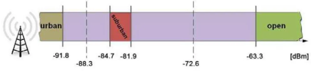
The minimum and the maximum propagation loss for each type of environment and for each TA are determined using equations (1), (4) and (5). The boundaries between different types of environments expressed through the level of the received signal for any value of TA parameter are obtained as

, . ,min/ max(TA) . ,max/ min(TA)

r env type t env type

n  n L , (7)

where L_{env type}_. _{, max/ min}(TA) is the maximum/minimum propagation loss for particular type of environment (urban, suburban or open) and particular TA parameter in dB, n_t is the base station transmitted power in dBm (precisely, this is the effective isotropic radiated power, PG_t _t where P_t is the transmitted power and G_t is the transmitter antenna gain) and n_{r env type}_, _. _{, min/ max}(TA) is minimum/maximum power of the received signal for particular type of environment and particular TA parameter, in dBm.

An illustration of the boundaries between different types of environments for TA5, n_t 50dB m, and h_t 30 m, which are some of the most common values, is shown in Fig. 1.

Fig. 1 –RSS value boundaries example for TA = 5.

(5)

finally determined, it follows estimation of the distance between a base station and a mobile station. The power of transmitted signal from the base station and received signal power are known, and we can easily reach propagation loss value L

r t

n  n L. (8)

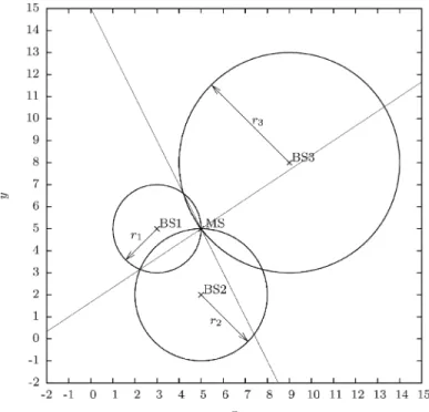
Once the value of L is determined, the propagation distance can be easily found applying some of the formulas (1), (4) or (5), depending on the type of environment. Parameter d is the only unknown in these terms. Having distances between the user (mobile terminal) and three or more base stations using a circular lateration we estimate location of the mobile station.

The circular lateration algorithm is illustrated in Fig. 2.

Fig. 2 –Circular lateration algorithm.

System of nonlinear equations derived from the circular lateration problem is:



 

2



2 2

MS BSk MS BSk k

x x  y y r . (9)

(6)

The system of original equations (9) is inconvenient to solve directly, it is nonlinear and likely inconsistent. The problem is greatly simplified by an algebraic transformation which results in linearization, finding the common intersecting point of circles (9) is reduced to finding the intersecting point of lines (Fig. 2), and location of the mobile station is determined as a solution of the system of linear equations [6]. The system of equations could be expressed in a matrix form

2 2 2 2 2 2

1 2 1 2 2 1 1 2 1 2

2 2 2 2 2 2

1 1 1 1 1

1 2

BS BS BS BS BS BS BS BS

MS

BS BSn BS BSn n BS BSn BS BSn

x x y y r r x x y y

x

y

x x y y r r x x y y

 

      

 

   

  _

   

 _{  }

 

        

   

   (10)

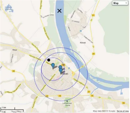
In practice, ideal consistency for all of the data is never the case (Fig. 3 and Fig. 4 show more common situation in practice [7]). For n3, this results in an inconsistent system of equations, i.e. all the lines specified by the equations do not share a common intersecting point. The situation is resolved solving (10) in the least squares sense. This introduces a heuristic, and such solution for the linear system is believed to be the best estimate of the mobile station location,



x_MS,y_MS



.

(7)

Fig. 4 –An example in suburban environment (balloons-base stations; circles-estimated distances; black '×'-estimated position; black dot-real position).

3 Different Scenarios and Experimental Results

In order to verify proposed algorithm, several simulation scenarios are performed. All of them use the same principle, but differ in some details: TA is read from all base stations in the region or only for the serving one; the antenna height and the base station transmitted power are set to the mean values or actual values are read from the operator database. A brief overview of various scenarios and their characteristics is given in Table 1. Each row represents a specific type of algorithm (scenario) and each column some of the required information.

(8)

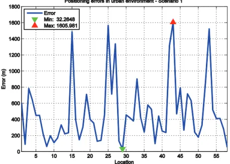
positioning error, we should pay attention to error fluctuation. It can be noticed that in some cases there is one or more locations with much larger positioning errors than the average. Scenario 4 in suburban environments and Scenario 1 in urban environment may serve as an illustration. They have very similar average error, but significantly different error values from location to location, as shown in Fig. 5 and Fig. 6.

Table 1

Overview of the scenarios.

BS

coordinates nr TA ht& nt

Using TA for calculating

distance

Scenario 1 Yes Yes All BS Average No

Scenario 2 Yes Yes Serving BS Average No

Scenario 2.1 Yes Yes Serving BS Average Yes

Scenario 3 Yes Yes All BS Real No

Scenario 4 Yes Yes Serving BS Real No

Scenario 4.1 Yes Yes Serving BS Real Yes

TA scenario Yes No All BS / Yes

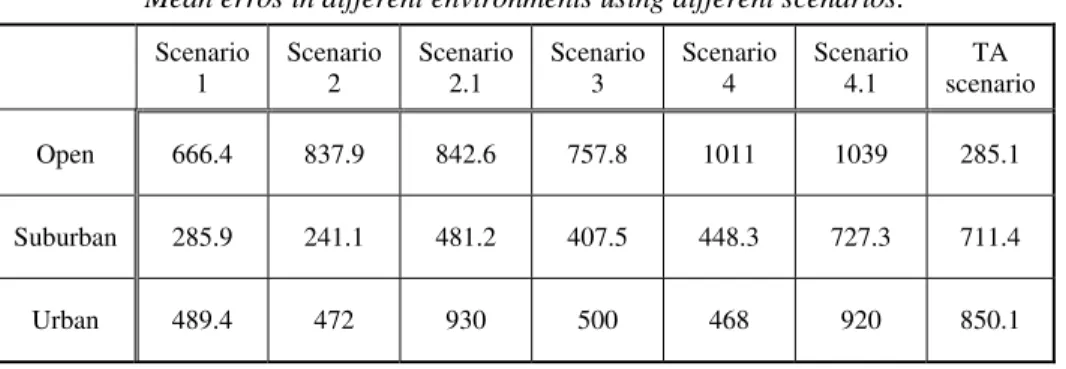
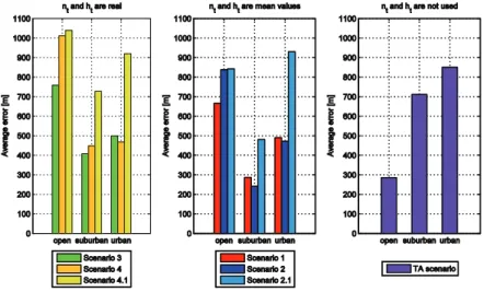
Table 2 presents the results, average positioning error (in meters) in different environments applying different scenarios (mentioned in Table 1).

Table 2

Mean erros in different environments using different scenarios.

Scenario 1

Scenario 2

Scenario 2.1

Scenario 3

Scenario 4

Scenario 4.1

TA scenario

Open 666.4 837.9 842.6 757.8 1011 1039 285.1

Suburban 285.9 241.1 481.2 407.5 448.3 727.3 711.4

(9)

Fig. 5 –Positioning error fluctuations in Scenario 4 for suburban environment.

(10)

base station transmission power and the base station antenna height (Scenarios 1, 2 and 2.1) and there are scenarios that read these data from the operator database (Scenario 3, 4 and 4.1). TA scenario does not use these data at all. This raises the question of availability such data and operators willingness to provide this information, regularly updated. In addition, from Table 2 it can be noticed that the first group of algorithms generally perform more precise positioning. Fig. 7 gives the chart that compares the results in this manner.

Fig. 7 – Comparison of the results I.

(11)

The second classification is based on available information about the TA parameter. There are two cases: TA parameters are known for all base stations within range, and TA parameter is known only for the serving base station. In order to obtain TA parameter for each BS, mobile station has to connect to each BS within the range (forced handover algorithm). This process requires a lot of time and resources, so Scenario 1 and Scenario 3 are time and power consuming, which is a very important fact. However, algorithms that fall into the second group (Scenario 2, 2.1, 4, 4.1) are usually less accurate than those in the first group. In Fig. 8, we can see the comparison of the results for these two groups of scenarios.

4 Conclusion

This paper presents a combined method of positioning in cellular systems by estimating the type of environment in which radio signals propagate. The developed algorithm was experimentally tested on the field in all three types of environments: urban, suburban and open. Different variants of the algorithm, called scenarios, are developed and we analyzed their results. From the results, we can observe that the algorithm performs very precise positioning in suburban environment, stable and reliable results in open environment, and unstable and diverse results in urban environment. When analyzing the efficiency of the algorithm, we need to pay attention to several important things. First, this algorithm does not require changes to the GSM network hardware or user handset, which means that it can be implemented quickly and inexpensively. Second, most of the scenarios have no major impact on a cellular network. Third, the algorithm provides the best results in suburban environments, which means in all cities except the largest ones.

There are many possibilities for future work. This algorithm represents only the initial idea and it gives results that are good enough to encourage further work. New propagation model can be improved or developed in order to achieve better results. Different classification types of environments certainly would have an effect on the final results. It would be interesting to analyze the relation between spatial distribution of the base stations and the positioning accuracy. That could lead to network being designed to be “positioning friendly” during cell planning. However, there are many ways in which this idea can be developed, in order to achieve more accurate positioning.

5 References

[1] 3GPP TS 22.071, release 8 (v8.0.0), Location Services (LCS) Service description; Stage 1, 2007, http://www.3gpp.org/ftp/Specs/archive/22_series/22.071.

(12)

[3] O. Bayrak, C. Temizyurek, M. Barut, O. Turkyilmaz, G. Gür: A Novel Mobile Positioning Algorithm Basedon Environment Estimation, 12th IEEE Workshop on Positioning, Navigation and Communication, WPNC’07, Hannover, Germany, 2007, pp. 211215. [4] J. S. Seybold: Introduction to RF Propagation, John Wiley & Sons, Inc., New Jersey, USA,

2005, pp. 134161.

[5] M. Hata: Empirical Formula for Propagation Loss in Land Mobile Radio Services, IEEE Transactions on Vehicular Technology, Vol. 29, No. 3, August 1980, pp. 317325.

[6] M. Simic, P. Pejovic: Positioning in Cellular Networks in Cellular Networks - Positioning, Performance Analysis, Reliability, A. Melikov (Ed.), In Tech, 2011, pp. 5176.