Multi-temporal airborne LIDAR-DEMs for glacier and permafrost mapping and monitoring

(1)

TCD

3, 383–414, 2009

Multi-temporal airborne LIDAR-DEMs

J. Abermann et al.

Title Page

Abstract Introduction

Conclusions References

Tables Figures

◭ ◮

Back Close

Full Screen / Esc

Printer-friendly Version

Interactive Discussion The Cryosphere Discuss., 3, 383–414, 2009

www.the-cryosphere-discuss.net/3/383/2009/ © Author(s) 2009. This work is distributed under the Creative Commons Attribution 3.0 License.

The Cryosphere Discussions

The Cryosphere Discussionsis the access reviewed discussion forum ofThe Cryosphere

Multi-temporal airborne LIDAR-DEMs for

glacier and permafrost mapping and

monitoring

J. Abermann1, A. Fischer2, A. Lambrecht2, and T. Geist3 1

Austrian Academy of Sciences, Commission for Geophysical Research, Vienna, Austria

2

Institute of Meteorology and Geophysics, University of Innsbruck, Innsbruck, Austria

3

FFG – Austrian Research Promotion Agency / ALR – Aeronautics and Space Agency, Vienna, Austria

Received: 9 June 2009 – Accepted: 22 June 2009 – Published: 1 July 2009

Correspondence to: J. Abermann (jakob.abermann@uibk.ac.at)

(2)

TCD

3, 383–414, 2009

J. Abermann et al.

Title Page

Tables Figures

◭ ◮

Back Close

Full Screen / Esc

Interactive Discussion

Abstract

The proposed method presents a simple and robust way to derive glacier extent by using multi-temporal high-resolution DEMs (digital elevation models) as a main data source. For glaciers that are not debris covered, we perform the glacier boundary delineation by analysing roughness differences between ice and its surroundings. A 5

promising way to distinguish dead ice, debris-covered ice or permafrost from its rocky surroundings is shown by taking elevation changes from DEMs of different dates into consideration. In case data has a high spatial and temporal resolution a good repre-sentation of the extent of debris cover and thus the overall ice covered area can be given. We use examples to show how potentially ambiguous areas can be treated 10

decisively by the additional qualitative analysis of aerial photographs. Problems and limitations are discussed in comparison with selected other remote sensing techniques and accuracies are quantified. For glaciers larger than 1 km2 an accuracy of±1% of the glacier area could be assessed. The errors of smaller glaciers do not exceed±5% of the glacier area.

15

1 Introduction

An overall glacier area and mass loss has been observed in the past decades through-out the world (e.g. Lemke et al., 2007; Dyurgerov and Meier, 2000; Haeberli, 1999; Oerlemans, 2005) as a result of climate change (e.g. Lemke et al., 2007; Trenberth et al., 2007). Many studies deal with mass-balance as well as run-o_ff modelling to 20

develop future scenarios of glacier extent and volume. These future states have large implications on the economy (water resources, tourism) of alpine regions. To quantify the recent changes and its current state in terms of area and volume, an actual dataset of glacier extent is thus mandatory. Additionally, a sound knowledge of the distribution of active rock glaciers is of interest for studies dealing with permafrost in a changing 25

(3)

TCD

3, 383–414, 2009

J. Abermann et al.

Title Page

Tables Figures

◭ ◮

Back Close

Full Screen / Esc

Interactive Discussion Mapping glacier extent and volume changes with remote sensing techniques is a

widely used and powerful method. Various studies show the potential and limitations of using satellite data (e.g. Andreassen et al., 2008; DeBeer and Sharp, 2007; Paul et al., 2007), airborne techniques as photogrammetry (e.g. Patzelt, 1980; W ¨url ¨ander et al., 2004) or LIDAR (light detetction and ranging, e.g. Baltsavias et al., 2001; Favey et al., 5

2002; Geist et al., 2003; Geist and St ötter, 2007; Geist and St ötter, 2009). Automatic or semi-automatic classification algorithms (Kodde et al., 2007; Paul et al., 2002; H öfle et al., 2007) are used to classify glacier areas.

For both, automatic and manual methods, the mapping of debris covered glacier areas is a general problem (e.g. Knoll and Kerschner, 2009; Paul et al., 2002). Fur-10

thermore, the automatic mapping of small glaciers is difficult (e.g. Paul et al., 2002). Lambrecht and Kuhn (2007) showed that 79% of all Austrian glaciers are smaller than 0.5 km2and 43% smaller than 0.1 km2.

These facts raised the need to develop a methodology for mapping and monitoring of all sizes of glaciers with and without debris cover and for the detection of rock glaciers. 15

In this paper, the use of high resolution DEMs for the monitoring of glacier and per-mafrost extent and volume changes is developed: The technique is applied to several test sites in the Austrian Alps, and compared to other mapping procedures.

2 Test sites and data

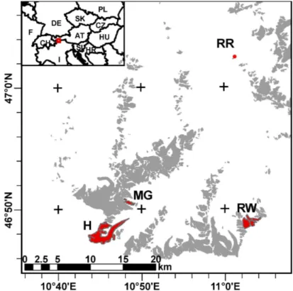
Three glaciers and one rock glacier in the ¨Otztal Alps were chosen as test sites. Hin-20

tereisferner in ¨Otztal Alps has been subject of extensive glaciological investigations for many years which results in a large number of DEMs, remote sensing data and field truth. Therefore, Hintereisferner was chosen as a test site for our method and com-pared with other remote sensing data. Since its tongue is partly debris covered we could evaluate the performance of the method on debris covered tongues. The nearby 25

(4)

TCD

3, 383–414, 2009

J. Abermann et al.

Title Page

Tables Figures

◭ ◮

Back Close

Full Screen / Esc

Interactive Discussion an example of Rotmoosferner. Reichenkar Rock glacier completes the test data set

with a well investigated rock glacier (Krainer et.al, 2002; Krainer and Mostler, 2000). Figure 1 shows the study area with glaciers in the ¨Otztal and Stubai Alps (grey) and the exemplarily discussed glaciers (red).

For all test sites, DEMs with 10 m cell size acquired in 1997 and high resolution 5

LIDAR-DEMs acquired in 2006 are available. The DEMs of 1997 were acquired during the compilation of the second Austrian glacier inventory by the means of digital pho-togrammetry (Lambrecht and Kuhn, 2007; W ¨url ¨ander and Eder, 1998). The LIDAR-DEMs of 2006 have been acquired by the regional government of Tyrol. The technical specifications of this LIDAR acquisition campaign are summarized in Table 1.

10

Another source of LIDAR-DEMs used covers a study area around Hintereisferner for which 14 DEMs have been produced between 2001 and 2007. Relative horizontal ac-curacies are better than 1 m and relative vertical acac-curacies better than 0.3 m according to Geist and St ¨otter (2007) where more technical specifications of this acquisition cam-paign are described. For the application of our method the survey flights 1 (10/2001), 15

11 (10/2004) and 12 (10/2005) have been chosen since they have been acquired in a similar time of the year (October) close to the minimum snow extent.

For the test site Hintereisferner, a direct comparison with other remote sensing data has been performed. Table 2 shows details on the acquisition dates of the data used and its accuracies as well as the spatial resolution.

20

3 Methodology

Ice thickness changes calculated from DEMs acquired at different timest₁andt₂can be used to gain important additional information for glacier extent mapping especially near the glacier tongue. Figure 2 shows the different temporal evolution of surface elevation schematically for a glacier without (a and c) and with debris cover (b and d). 25

(5)

TCD

3, 383–414, 2009

J. Abermann et al.

Title Page

Tables Figures

◭ ◮

Back Close

Full Screen / Esc

Interactive Discussion thickness loss is reached near the glacier margin at the time when the newer DEM was

acquired (t₂, indicator 2).

A glacier with debris cover, as indicated schematically in Fig. 2b and d, evolves differently due to the fact that debris cover reduces ablation compared to bare ice (e.g. Kirkbride and Warren, 1999). For this reason, elevation differences between t₁ 5

andt₂ are significantly smaller at the debris covered parts (between indicators 3 and 4) and instantly increase where debris cover meets bare ice (from 4 upwards).

We used these differences to gain information on the occurrence and, depending on the time between the acquired DEMs, the extent of debris-cover.

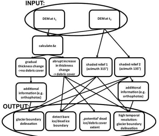
The work-flow of the applied methodology is highlighted schematically in Fig. 3. In 10

a first step we calculated elevation differences between the two available DEMs of the respective region. In addition to that, we calculated two hillshades with different azimuth-angles for illumination (315◦ and 135◦) through the ESRI-Software ArcMap to optimally visualize contrasts in different aspects. Taking advantage of the already ex-isting glacier inventory of a former date (Lambrecht and Kuhn, 2007) we then analysed 15

qualitatively in which way ice thickness has evolved from the former glacier terminus position upwards according to Fig. 2. The existence of former glacier boundaries is not mandatory but saves time since it shows where to expect glacier covered areas. Nevertheless, even if a former dataset of glacier boundaries exists, testing it with the difference raster is advisable. This is to avoid that a glacier that had not been captured 20

in a previous study is not captured in a new study either.

In the case a gradual increase in ice thickness loss is observed from the former glacier tongue upwards, we set the glacier boundary directly by digitising the strongest roughness change in the hillshades.

If an abrupt increase in ice thickness loss can be detected, we use the hillshades to 25

(6)

TCD

3, 383–414, 2009

J. Abermann et al.

Title Page

Tables Figures

◭ ◮

Back Close

Full Screen / Esc

Interactive Discussion thickness change has occurred.

In accumulation zones of glaciers, surface elevation changes are much smaller. We therefore could only partly take advantage of the difference raster and thus used the roughness changes in the hillshades as well as orthophotos to map the glacier extent in these areas.

5

4 Results

We now highlight the results of the applied method with exemplarily chosen reference glaciers of di_fferent characteristics.

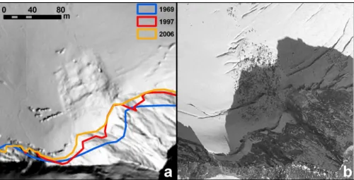
4.1 Debris-free glacier tongues – e.g. Mittlerer Guslarferner

The small (0.5 km2), debris-free Mittlerer Guslarferner shows a gradual ice thickness 10

loss from the former glacier margin upwards (Fig. 4a); An optimal delineation of the glacier extent is performed by following the pronounced roughness changes in the hillshades as visualized in Fig. 4b.

4.2 Accumulation zone – e.g. Rotmoosferner

In large parts of the accumulation area we achieved good results by analysing rough-15

ness changes of the hillshades and could thus set the glacier boundary well. As sug-gested in UNESCO (1970) we included adjacent snow-covered areas to the glacier surface area. The acquisition date of the LIDAR-DEMs (October and late August, see Table 2) is optimal since it is close to the minimum snow cover in the Alps. In some cases also in the lower parts of the accumulation zone the analysis of surface eleva-20

(7)

TCD

3, 383–414, 2009

J. Abermann et al.

Title Page

Tables Figures

◭ ◮

Back Close

Full Screen / Esc

Interactive Discussion simply analysing the hillshade of the DEM. Also the analysis of the surface elevation

changes did not result in a distinct answer since surface elevation changes were very small in this region. In this case a qualitative comparison with an aerial photograph of 2003 taken by the regional government of Tyrol (Tirismaps, 2009) gives a good hint be-cause crevasse patterns can be seen in this debris- or rock-covered part of the glacier 5

(Fig. 5b).

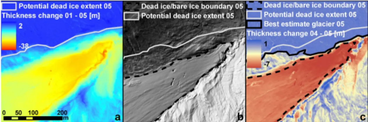
4.3 Debris-covered glacier tongues – e.g. Hintereisferner

In case we identified an abrupt increase in elevation loss around the former glacier boundary we followed a di_fferent work-flow as indicated in Fig. 3. An example of this is given in Fig. 6 for Hintereisferner’s tongue. Figure 6a shows the calculated diff er-10

ences between 2001 and 2005 and allows thus to define a potential dead ice extent by including all areas with a significant change. However, as UNESCO (1970) suggests, adjacent debris covered areas and dead ice bodies have to be included in glacier inven-tories. Therefore we included the areas where a significant elevation change occurred to a so-called “potential” glacier area. The significance of the potential glacier area de-15

pends on the temporal resolution of the multi-temporal DEMs. In case the two DEMs used have been acquired a long time apart from each other (e.g. decades) and during this period a significant ice volume loss has occurred, it can well be that ice that was stored beneath the debris cover has partly melted out by the time of the second acqui-sition date. In this case the additional use of multi-temporal DEMs should be seen as 20

(8)

TCD

3, 383–414, 2009

J. Abermann et al.

Title Page

Tables Figures

◭ ◮

Back Close

Full Screen / Esc

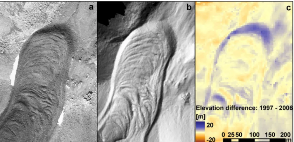
4.4 Rock glaciers – e.g. Reichenkar Rock glacier

Remote sensing techniques are not only applicable for the mapping and monitoring of glaciers and their changes but also of permafrost (e.g. K ¨a ¨ab, 2008a).

Figure 7 shows an example of Reichenkar rock glacier. We use it as an example to show that orthophotos (7a, 1997) as well as hillshades of high-resolution LIDAR-DEMs 5

(7b, 2006) are appropriate datasets to derive rock-glacier’s extents when they have a distinct snout. Both datasets result in a similar accuracy for the mapping of rock glacier extents. The calculation of volume changes from two successive DEMs is shown in Fig. 7c. The snout has advanced by ca. 25 m which can be seen in the elevation differences. In case two successive LIDAR-DEMs existed from this area, accurate 10

mapping also of the upper areas of rock glaciers could be done as demonstrated with the debris-covered areas on Hintereisferner (Fig. 6). So far, subsequent LIDAR-DEMs are only available for a test region around Hintereisferner. Since elevation changes on rock glaciers are usually small apart from changes at the snout (e.g. Schneider and Schneider, 2001) a sequence of very accurate DEMs would be necessary to investigate 15

volume changes over the entire rock glacier area. However, the difference raster can be taken as a method to distinguish active from fossile rock glaciers.

4.5 Accuracy

Assessing the accuracy of the proposed method quantitatively we point out that inter-pretation uncertainty is higher than horizontal errors of the DEMs (Table 2), therefore 20

we neglected the latter. To estimate errors introduced by interpretation we first com-pared the results of two different persons for some glaciers. The deviance was less than 1% of the total area. Moreover, we evaluated some glaciers randomly out of dif-ferent size classes and produced one maximum and one minimum extent by including all ambiguous areas and excluding them, respectively. The resulting glacier areas have 25

(9)

TCD

3, 383–414, 2009

J. Abermann et al.

Title Page

Tables Figures

◭ ◮

Back Close

Full Screen / Esc

Interactive Discussion the best estimate for the accuracy of the methodology.

5 Discussion

5.1 Hillshades and differences: cell-size

The influence of the cell-size of the DEM on the quality of the glacier boundary delin-eation with high-resolution DEMs as a main data source is highlighted in Figs. 8 and 5

9. We calculated three hillshades out of differently resampled DEMs (Fig. 8 a–c) of the same extent as in Fig. 4. The derivation of glacier boundaries by using the rough-ness changes out of hillshades as a main criterion is only applicable for DEMs that exist at a resolution better than 5 m. 1 m-DEMs are optimal and allow to omit the use of orthophotos or any other additional information for glaciers without debris-cover. A 10

cell-size of 20 m or higher does not resolve roughness changes adequately (8 b and c). Figure 9 shows analogously the calculated ice thickness changes out of differently resampled DEMs on Hintereisferner’s tongue (same extent as Fig. 6). The di_fferences between the rocky surroundings, the covered part of the tongue and the debris-free ice is visible up to the 50 m resolution but since differences between the surface 15

characteristics are small (compare noise in rocky surroundings with debris-covered part in 9b and c no significant conclusions can be drawn for cell-sizes larger than 5 m.

5.2 Exemplary comparison to other remote sensing techniques

Figure 10 shows an overview of the pixel size and the vertical accuracy of the discussed remote sensing data as well as orders of magnitudes of overall mean annual thickness 20

(10)

TCD

3, 383–414, 2009

J. Abermann et al.

Title Page

Tables Figures

◭ ◮

Back Close

Full Screen / Esc

Interactive Discussion box (e.g. orthophotos and Landsat data) do not include topographic information. The

applicability of ice thickness changes for the detection of glacier boundaries depends on the magnitude of elevation change (time difference, climate signal) compared to the sum of the vertical accuracies of the used DEMs. The use of LIDAR-DEMs together with the DEM 1997 is thus a comparably accurate option both in terms of the achieved 5

pixel size as well as vertical accuracies. In the next parts, we will use the example of Hintereisferner’s debris-covered tongue to qualitatively compare glacier boundary de-lineation with very high resolution DEMs (e.g. LIDAR) with other remote sensing data often used for this purpose.

5.2.1 Aerial photogrammetry

10

Many studies in the past use photogrammetrically derived orthophotos of varying pixel-sizes (e.g. 1 m: Lambrecht and Kuhn, 2007) as the main data source to obtain the glacier extent. This is a good method for debris-free glaciers and still provides the best results for glacier mapping in the accumulation zone where surface elevation changes are small. Photogrammetry also includes the opportunity to produce high-quality DEMs 15

although their accuracy may be reduced in the accumulation zone due to oversaturation of the acquired images. Geist et al. (2003) and W ¨url ¨ander et al. (2004) pointed this out as a main advantage of LIDAR for glaciers.

Figure 11 shows an orthophoto of 2003 of Hintereisferner’s tongue. In the debris-covered area it is not possible to detect the glacier boundary decisively simply by 20

(11)

TCD

3, 383–414, 2009

J. Abermann et al.

Title Page

Tables Figures

◭ ◮

Back Close

Full Screen / Esc

5.2.2 Multispectral remote sensing

The use of Landsat scenes as a main data source is widespread in literature and allows a mainly automatic glacier boundary detection (e.g. Andreassen et al., 2008; Paul et al., 2002). The pixel-size is 30 m for the relevant channels. Figure 12 shows the example of a Landsat-scene around Hintereisferner (NASA, 2004). With the combination of 5

channels 4, 5 and 6 glacier ice can be distinguished from its rocky surroundings (Rott and Markl, 1989). The close-up rectangle in the upper left corner of Fig. 12 shows the discussed area of Fig. 6. Details as indicated in Fig. 6 (dead ice, detailed glacier boundary) are not possible to be detected with this data.

If Landsat-scenes are in use for glacier monitoring, additional remote sensing data 10

have to be taken into account for the computation of DEMs in case volume changes are of interest.

SPOT

SPOT-Scenes reach a pixel-size of 2.5–20 m in various wavelengths (CNES, 2009). Figure 13 shows an example of the same study area again with a close-up rectangle in 15

the upper left corner. Glacier boundary can be delineated well for debris-free glaciers although additional information as (a sequence of) high-resolution DEMs is eligible to enhance accuracies in ambiguous areas (e.g. debris-cover).

IKONOS

The IKONOS-satellite provides images of different bands in the visible range with 20

comparable horizontal resolutions as the orthophotos used in this study (1 m). Sharov and Etzold (2007) evaluated IKONOS-data of Hintereisferner and derived horizontal accuracies of 17 m. Figure 14 shows a panchromatic IKONOS-scene of Hintereis-ferner’s tongue of August 2003 (Sharov and Etzold, 2007). The potential to delineate the debris-cover extent is limited, comparable to the example of the orthophoto shown 25

(12)

TCD

3, 383–414, 2009

J. Abermann et al.

Title Page

Tables Figures

◭ ◮

Back Close

Full Screen / Esc

Interactive Discussion ASTER

The ASTER-satellite provides images of cell-sizes between 15 and 90 m for wavelengths between 0.52 and 11.65µm. The accuracies of the DEMs calculated from ASTER data (K ¨a ¨ab, 2008b) lack the accuracy to monitor short-term changes (e.g. years) of glaciers or permafrost. Concerning glacier boundary delineation similar 5

success as well as limitations as shown for Landsat before occur due to its comparably large cell-size (K ¨a ¨ab et al., 2002).

6 Conclusions

The comparison of multi-temporal DEMs with a relative vertical accuracy significantly better than the ice thickness change over the investigated period enhance the accu-10

racy of mapping glacier boundaries. The method is well-suited for study areas with a manageable extent where an accurate knowledge of glacier area and volume change is needed since it requires considerable manual digitisation effort. A great advantage compared to other remote sensing techniques is high accuracy for the delineation of small glaciers (e.g. <0.5 km2). The combination of additional information (e.g. multi-15

temporal DEMs and orthophotos) or other remote sensing data further improves the result.

The better the vertical accuracy and the horizontal resolution of the DEMs is, the shorter the time period between the acquisition of the DEMs can be chosen.

In a climate closer to a steady state of glaciers than today’s climate, the application 20

of this mapping procedure would be less successful since surface elevation changes would be smaller.

The accuracy of the glacier boundary delineation is higher in areas with large eleva-tion changes, i.e. low elevaeleva-tions and bare ice.

There is also a high potential in using multi-temporal DEMs to map and monitor 25

(13)

TCD

3, 383–414, 2009

J. Abermann et al.

Title Page

Tables Figures

◭ ◮

Back Close

Full Screen / Esc

Interactive Discussion into account. Long-term elevation changes allow also the distinction of active and

fossile rock glaciers.

Compared to other remote sensing techniques, the use of multi-temporal LIDAR-DEMs implies the advantage of giving the possibility to derive glacier boundaries as well as volume change both in a high resolution without data gaps caused by the imag-5

ing geometry.

The application of multi-temporal DEMs for the detection of debris-covered glaciers in case large stone or debris mass turnovers which could have balanced or dominated possible vertical ablation depends on the horizontal and vertical resolution of the DEMs. The use of multi-temporal DEMs will gain importance in future glaciological applica-10

tions since the number of high-resolution DEMs is increasing and airborne as well as satellite data reaches higher accuracies. The prospected future climate change (Tren-berth et al., 2007) will result in a continuing glacier volume and area loss and thus this method may be extended further.

Acknowledgements. This study was funded by the Commission for Geophysical Research, 15

Austrian Academy of Science. The LIDAR-DEM 2006 was acquired by the Regional Govern-ment of Tyrol. The authors would like to thank M. Kuhn and C. Knoll for their comGovern-ments, L. Raso for proof-reading the paper, M. Juen for his help with Fig. 2 and M. Attwenger for providing in-formation on the LIDAR-DEM.

References

20

Abermann, J., Lambrecht, A., Fischer, A., and Kuhn, M.: Quantifying changes and trends in glacier area and volume in the Austrian ¨Otztal Alps (1969–1997–2006), The Cryosphere Discuss., 3, 415–441, 2009,

http://www.the-cryosphere.net/3/415/2009/.

Andreassen, L. M., Paul, F., K ¨a ¨ab, A., and Hausberg, J. E.: Landsat-derived glacier inventory 25

for Jotunheimen, Norway, and deduced glacier changes since the 1930s, The Cryosphere, 2, 131–145, 2008,

(14)

TCD

3, 383–414, 2009

J. Abermann et al.

Title Page Abstract Introduction Conclusions References Tables Figures ◭ ◮ ◭ ◮ Back Close

Full Screen / Esc

Interactive Discussion Baltsavias, E. P., Favey, E., Bauder, A., B ¨osch, H., and Pateraki, M.: Digital Surface

Mod-elling by Airborne Laser Scanning and Digital Photogrammetry for Glacier Monitoring, Pho-togramm. Rec., 17(98), 243–273, 2001.

CNES: http://www.cnes.fr/web/CNES-en/1415-spot.php, last access: 29 May 2009.

DeBeer, C. M. and Sharp, M. J.: Recent changes in glacier area and volume within the southern 5

Canadian Cordillera, Ann. Glaciol., 46, 215–221, 2007.

Dyurgerov, M. B. and Meier, M. F.: Twenthieth century climate change: Evidence from small glaciers, PNAS, 97(4), 1406–1411, 2000.

Favey, E., Wehr, A., Geiger, A., and Kahle, H.-G.: Some examples of European activities in airborne laser techniques and an application in glaciology, J. Geodyn., 34, 347–355, 2002. 10

Fischer, A., Markl, G., and Dreiseitl, E.: Reanalysis and interpretation of 50 years of direct mass balance of Hintereisferner, Austria, submitted, Global Planet. Change, 2009.

Geist, T., Lutz, E., and St ¨otter, J.: Airborne laser scanning technology and its potential for applications in glaciology, International Archives of Photogrammetry, Remote Sensing and Spatial Information Science, Vol. XXXIV/3/W13, 101–106, 2003.

15

Geist, T., Elvehoy, H., Jackson, M. and St ¨otter, J.: Investigations on intra-annual elevation changes using multi-temporal airborne laser scanning data – case study Engabreen, Norway, Ann. Glaciol., 42, 195–201, 2005.

Geist, T. and St ¨otter, J.: Documentation of glacier surface elevation change with multi-temporal airborne laser scanner data – case study: Hintereisferner and Kesselwandferner, Tyrol, Aus-20

tria, Zeitschrift f ¨ur Gletscherkunde und Glazialgeologie, 41, 77–106, 2007.

Geist, T. and St ¨otter, J.: Laser scanning in glacier studies, in: Remote Sensing of Glaciers, edited by: Pellika, P. and Rees, W. G., Taylor and Francis Ltd., London, 2009.

Haeberli, W., Frauenfelder, R., Hoelzle, M., and Maisch, M.: On rates and acceleration trends of global glacier mass changes, Geogr. Ann., 81(A(4)), 585–591, 1999.

25

H ¨ofle, B., Geist, T., Rutzinger, M., and Pfeifer, N.: Glacier surface segmentation using airborne laser scanning point cloud and intensity data, International Archives of Photogrammetry, Remote Sensing and Spatial Information Sciences, Vol. XXXVI/3, 195–200, 2007.

K ¨a ¨ab, A.: Remote Sensing of Permafrost – related Problems and Hazards, Permafrost Periglac., 19, 107–136, 2008a.

30

(15)

TCD

3, 383–414, 2009

J. Abermann et al.

Title Page Abstract Introduction Conclusions References Tables Figures ◭ ◮ ◭ ◮ Back Close

Full Screen / Esc

Interactive Discussion K ä äb, A., Paul, F., Maisch, M., and H äberli, W.: The new remote-sensing-derived Swiss Glacier

Inventory: II, First results, Ann. Glaciol., 34, 362–366, 2002.

Kirkbride, M. P. and Warren, C. R.: Tasman Glacier, New Zealand: 20th-century thinning and predicted calving retreat, Global Planet. Change, 22, 11–28, 1999.

Knoll, C. and Kerschner, H.: A glacier inventory for South Tyrol, Italy, based on airborne laser 5

scanner data, Ann. Glaciol., 50(53), accepted, 2009.

Kodde, M., Pfeiffer, N., Gorte, B., Geist, T., and H ¨ofle, B.: Automatic Glacier Surface Analysis from Airborne Laser Scanning, ISPRS Workshop Laser Scanning 2007, XXXVI Part 3/W52, 221–226, 2007.

Krainer, K. and Mostler, W.: Reichenkar Rock Glacier, a glacial derived debris-ice system in 10

the Western Stubai Alps, Austria, Permafrost Periglac., 11, 267–275, 2000.

Krainer, K. , Mostler, W., and Span, N.: A glacier derived, ice-cored rock glacier in the western Stubai Alps (Austria): Evidence from exposures and ground penetrating radar investigation, Zeitschrift f ¨ur Gletscherkunde und Glazialgeologie, 38(1), 21–34, 2002.

Lambrecht, A. and Kuhn, M.: Glacier changes in the Austrian Alps during the last three 15

decades, derived from the new Austrian glacier inventory, Ann. Glaciol., 46, 177–184, 2007. Lemke, P., Ren, J., Alley, R. J. et al.: Observations: Changes in Snow, Ice and Frozen Ground,

in: Climate Change 2007: The Physical Science Basis, edited by: Solomon, S., Qin, D., Manning, M. et al., Contribution of Working Group I to the Fourth Assessment Report of the Intergovernmental Panel on Climate Change, Cambridge University Press, Cambridge, UK 20

and New York, NY, USA, 2007.

NASA Landsat Program, Landsat ETM+scene LE71930272004254ASN01, L1T, USGS, Aus-tria/Italy, 10.09.2004, 2004.

Oerlemans, J.: Extracting a climate signal from 169 glacier records, Science, 308, 675–677, 2005.

25

Patzelt, G.: The Austrian glacier inventory: status and first results. Riederalp Workshop 1978 – World Glacier Inventory, IAHS, 1980.

Paul, F., K ä äb, A., Maisch, M., Kellenberger, T. W., and H äberli, W.: The new remote-sensing-derived Swiss Glacier Inventory: I. methods, Ann. Glaciol., 34, 355–361, 2002.

Paul, F., K ¨a ¨ab, A., and Haeberli, W.: Recent glacier changes in the Alps observed from satellite: 30

Consequences for future monitoring strategies, Global Planet. Change, 56(1/2), 111–122, 2007.

(16)

TCD

3, 383–414, 2009

J. Abermann et al.

Title Page

Tables Figures

◭ ◮

Back Close

Full Screen / Esc

Interactive Discussion Proceedings of a workshop on Landsat Thematic Mapper applications, ESA, SP–1102, 3–

12, 1999.

Schneider, B. and Schneider, H.: Zur 60j ährigen Messreihe der kurzfristigen Geschwindigkeitsschwankungen am Blockgletscher im Äußeren Hochebenkar, Ötztaler Alpen, Tirol, Zeitschrift f ür Gletscherkunde und Glazialgeologie, 37(1), 1–33, 2001.

5

Sharov, A. and Etzold, S.: Stereophotogrammetric mapping and cartometric analysis of glacier changes using IKONOS imagery, Zeitschrift f ¨ur Gletscherkunde und Glazialgeologie, 41, 107–130, 2007.

Spot Image: http://www.spotimage.fr/web/en/811-spot-dem.php, last access: 29 May 2009. Trenberth, K. E., Jones, P. D., Ambenje, P. et al.: Observations: Surface and Atmospheric 10

Climate Change, in: Climate Change 2007: The Physical Science Basis, edited by: Solomon, S., Qin, D., Manning, M. et al., Contribution of Working Group I to the Fourth Assessment Report of the Intergovernmental Panel on Climate Change, Cambridge University Press, Cambridge, UK and New York, NY, USA, 2007.

Tirismaps: https://portal.tirol.gv.at, last access: 29 May 2009. 15

UNESCO: Perennial ice and snow masses: a guide for compilation and assemblage of data for a world inventory, Technical Paper Hydrology 1. UNESCO/IASH, 1970.

W ürl änder, R. and Eder, K.: Leistungsf ähigkeit aktueller photogrammetrischer Auswertemeth-oden zum Aufbau eines digitalen Gletscherkatasters, Zeitschrift f ür Gletscherkunde und Glazialgeologie, 35, 167–185, 1998.

20

(17)

TCD

3, 383–414, 2009

J. Abermann et al.

Title Page

Tables Figures

◭ ◮

Back Close

Full Screen / Esc

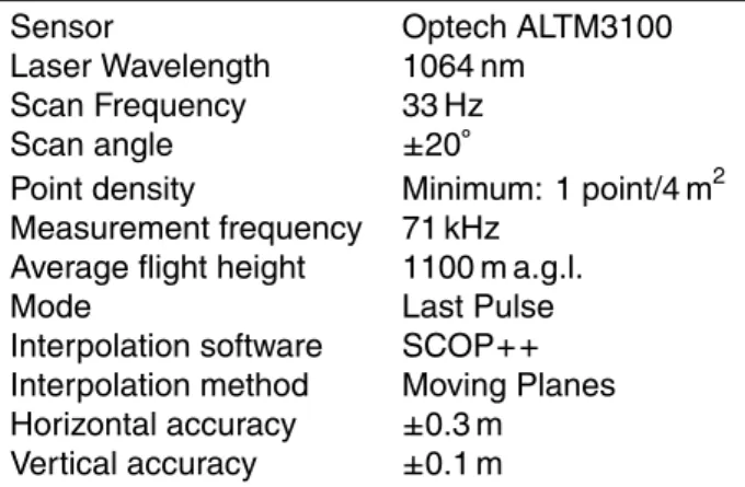
Table 1.Summary of technical specifications of the LIDAR acquisition campaign of the regional governement of Tyrol, 2006.

Sensor Optech ALTM3100

Laser Wavelength 1064 nm Scan Frequency 33 Hz

Scan angle _±20◦

Point density Minimum: 1 point/4 m2 Measurement frequency 71 kHz

Average flight height 1100 m a.g.l.

Mode Last Pulse

Interpolation software SCOP++ Interpolation method Moving Planes Horizontal accuracy ±0.3 m

(18)

TCD

3, 383–414, 2009

J. Abermann et al.

Title Page

Tables Figures

◭ ◮

Back Close

Full Screen / Esc

Table 2. Summary of the acquisition dates as well as resolutions and accuracies of the data used in this study. For references concerning the accuracies of LIDAR and Photogrammetry see above, Landsat, SPOT and IKONOS see Sect. 5.2.2.

Source data Date Band Horizontal Horizontal Vertical resolution [m] accuracy accuracy

[m] [m]

Aerial 11/9/1997 10 1 1.9

photography

LIDAR 11/10/2001 1 <1 <0.3

LIDAR 5/10/2004 1 <1 <0.3

LIDAR 12/10/2005 1 <1 <0.3

LIDAR 23/08/2006 1 0.3 0.1

Landsat 10/09/2004 4,5,6 H 30 ca. 30 –

SPOT 17/07/1999 panchromatic 10 15 10

(19)

TCD

3, 383–414, 2009

J. Abermann et al.

Title Page

Tables Figures

◭ ◮

Back Close

Full Screen / Esc

(20)

TCD

3, 383–414, 2009

J. Abermann et al.

Title Page

Tables Figures

◭ ◮

Back Close

Full Screen / Esc

Interactive Discussion Figure 2: Schematic model of surface evolution of a debris-free (a) versus a debris covered

(21)

TCD

3, 383–414, 2009

J. Abermann et al.

Title Page

Tables Figures

◭ ◮

Back Close

Full Screen / Esc

DEM at t1

high temporal resoluon: glacier boundary

delineaon abrupt increase

in thickness change -> debris cover gradual

thickness change ->no debris cover

shaded relief 1 (azimuth 315°) calculate Δz

DEM at t2

shaded relief 2 (azimuth 135°)

glacier boundary delineaon

‚potenal‘ dead ice/debris cover

extent detect bare

ice/dead ice boundary addional

informaon (e.g. orthophotos)

addional informaon (e.g.

orthophotos)

INPUT:

OUTPUT:

(22)

TCD

3, 383–414, 2009

J. Abermann et al.

Title Page

Tables Figures

◭ ◮

Back Close

Full Screen / Esc

Fig. 4. Elevation change 1997–2006 with the glacier boundary of 1997 (dotted) on Mittlerer Guslarferner. To calculate elevation changes we resampled the DEM 2006 to 5 m cell-size(a).

(23)

TCD

3, 383–414, 2009

J. Abermann et al.

Title Page

Tables Figures

◭ ◮

Back Close

Full Screen / Esc

Fig. 5.Ambiguous glacier boundary at Rotmoosferner’s firn area displayed as a hillshade of the 2006 DEM (azimuth angle: 315◦_{) with glacier margins of 1996 (black, dashed), 1997 (orange,}

(24)

TCD

3, 383–414, 2009

J. Abermann et al.

Title Page

Tables Figures

◭ ◮

Back Close

Full Screen / Esc

Fig. 6.In(a)the ice thickness changes between 2001 and 2005 are shown in a colour scheme. A potential dead ice extent can be delineated by considering changed surface elevations. The calculated hillshade from the 2005 DEM is shown in(b). With this information it is only possible to detect the boundaries between dead ice and bare ice. The use of DEMs with a short time interval (e.g. 1 year) allows the detection of dead ice and thus the general ice-covered area well

(25)

TCD

3, 383–414, 2009

J. Abermann et al.

Title Page

Tables Figures

◭ ◮

Back Close

Full Screen / Esc

(26)

TCD

3, 383–414, 2009

J. Abermann et al.

Title Page

Tables Figures

◭ ◮

Back Close

Full Screen / Esc

(27)

TCD

3, 383–414, 2009

J. Abermann et al.

Title Page

Tables Figures

◭ ◮

Back Close

Full Screen / Esc

Fig. 9. Calculated ice thickness changes out of differently resampled DEMs with 5 m(a), 20 m

(28)

TCD

3, 383–414, 2009

J. Abermann et al.

Title Page

Tables Figures

◭ ◮

Back Close

Full Screen / Esc

(29)

TCD

3, 383–414, 2009

J. Abermann et al.

Title Page

Tables Figures

◭ ◮

Back Close

Full Screen / Esc

(30)

TCD

3, 383–414, 2009

J. Abermann et al.

Title Page

Tables Figures

◭ ◮

Back Close

Full Screen / Esc

(31)

TCD

3, 383–414, 2009

J. Abermann et al.

Title Page

Tables Figures

◭ ◮

Back Close

Full Screen / Esc

(32)

TCD

3, 383–414, 2009

J. Abermann et al.

Title Page

Tables Figures

◭ ◮

Back Close

Full Screen / Esc