Spatial patterns in glacier area and elevation changes from 1962 to 2006 in the monsoon-influenced eastern Himalaya

(1)

TCD

8, 3949–3998, 2014

Spatial patterns in glacier area and elevation changes

from 1962 to 2006

A. Racoviteanu et al.

Title Page

Abstract Introduction

Conclusions References

Tables Figures

◭ ◮

Back Close

Full Screen / Esc

Printer-friendly Version

Interactive Discussion

Discussion

P

a

per

|

Discus

sion

P

a

per

|

Discussion

P

a

per

|

Discussion

P

a

per

The Cryosphere Discuss., 8, 3949–3998, 2014 www.the-cryosphere-discuss.net/8/3949/2014/ doi:10.5194/tcd-8-3949-2014

This discussion paper is/has been under review for the journal The Cryosphere (TC). Please refer to the corresponding final paper in TC if available.

Spatial patterns in glacier area and

elevation changes from 1962 to 2006 in

the monsoon-influenced eastern Himalaya

A. Racoviteanu1, Y. Arnaud1,2, M. Williams3, and W. F. Manley4

1

Laboratoire de Glaciologie et Géophysique de l’Environnement, 54, rue Molière, Domaine Universitaire, BP 96 38402, Saint Martin d’Hères cedex, France

2

Laboratoire d’étude des Transferts en Hydrologie et Environnement, BP 53 38401, Saint Martin d’Hères cedex, France

3

Department of Geography and Institute of Arctic and Alpine Research, University of Colorado, Boulder, CO 80309, USA

4

Institute of Arctic and Alpine Research, University of Colorado, Boulder, CO, 80309, USA

Received: 2 April 2014 – Accepted: 15 April 2014 – Published: 18 July 2014

Correspondence to: A. Racoviteanu (racovite@gmail.com)

(2)

TCD

8, 3949–3998, 2014

from 1962 to 2006

Title Page

Tables Figures

◭ ◮

Back Close

Full Screen / Esc

Discussion

P

a

per

|

Discus

sion

P

a

per

|

Discussion

P

a

per

|

Discussion

P

a

per

|

Abstract

This study presents spatial patterns in glacier area and elevation changes in the monsoon-influenced part of the Himalaya (eastern Nepal and Sikkim) at multiple spatial scales. We combined Corona KH4 and topographic data with more recent remote-sensing data from Landsat 7 Enhanced Thematic Mapper Plus (ETM+_{), the}

5

Advanced Spaceborne Thermal Emission Radiometer (ASTER), QuickBird (QB) and WorldView-2 (WV2) sensors. We present: (1) spatial patterns of glacier parame-ters based on a new “reference” geospatial Landsat/ASTER glacier inventory from

∼2000; (2) changes in glacier area (1962–2006) and their dependence on

topo-graphic variables (elevation, slope, aspect, percent debris cover) as well as climate

10

variables (solar radiation and precipitation), extracted on a glacier-by-glacier basis and (3) changes in glacier elevations for debris-covered tongues and their relation-ship to surface temperature extracted from ASTER data. Glacier mapping from 2000 Landsat/ASTER yielded 1463 km2±88 km2 total glacierized area in Nepal (Tamor

basin) and Sikkim (Zemu basin), parts of Bhutan and China, of which we estimated

15

569 km2±34 km2to be located in Sikkim. Supraglacial debris covered 11 % of the total

glacierized area, and supraglacial lakes covered about 5.8 % of the debris-covered area. Based on analysis of high-resolution imagery, we estimated an area loss of

−0.24 %±0.08 % yr−1 from the 1960’s to the 2010’s, with a higher rate of retreat in

the last decade (−0.43 % yr−1±0.9 % from 2000 to 2006) compared to the previous

20

decades (−0.20 % yr−1±0.16 % from 1962 to 2000). Retreat rates of clean glaciers

were −0.7 % yr−1, almost double than those of debris-covered glaciers (−0.3 % yr−1).

Debris-covered tongues experienced an average lowering of −30.8 m±39 m from

1960’s to 2000’s (−0.8 m±0.9 m yr−1), with enhanced thinning rates in the upper part

of the debris covered area, and overall thickening at the glacier termini.

(3)

TCD

8, 3949–3998, 2014

from 1962 to 2006

Title Page

Tables Figures

◭ ◮

Back Close

Full Screen / Esc

Discussion

P

a

per

|

Discus

sion

P

a

per

|

Discussion

P

a

per

|

Discussion

P

a

per

1 Introduction

Himalayan glaciers have aroused a lot of concern in the last few years, particularly with respect to glacier area and elevation changes and their consequences for the regional water cycle (Immerzeel et al., 2010, 2012; Kaser et al., 2010; Racoviteanu et al., 2013). Remote sensing techniques helped improve estimates of glacier area changes

(Ba-5

jracharya et al., 2007; Bolch, 2007; Bolch et al., 2008a; Bhambri et al., 2010; Kamp et al., 2011), glacier lake changes (Wessels et al., 2002; Bajracharya et al., 2007; Bolch et al., 2008b; Gardelle et al., 2011) and region-wide glacier mass balance (Berthier et al., 2007; Bolch et al., 2011; Kääb et al., 2012; Gardelle et al., 2013), but signifi-cant gaps do remain. The new global Randolph inventory (Pfeﬀ_{er et al., 2014) provides}

10

a global dataset of glacier outlines intended for large-scale studies; in some regions the quality varies and the outlines may not be suitable for detailed regional analysis of glacier parameters. Among recent glacier inventories, we cite those in the western part of the Himalaya (Bhambri et al., 2011; Kamp et al., 2011; Frey et al., 2012), and a few in the eastern Himalaya (Bahuguna, 2001; Krishna, 2005; Bajracharya and Shrestha,

15

2011; Basnett et al., 2013). Parts of the monsoon-influenced eastern Himalaya (the eastern extremity of Nepal, Sikkim and Bhutan) still lack comprehensive, multi-temporal glacier data needed for accurate change detection. The use of remote sensing for glacier mapping in this area is limited by frequent cloud cover and sensor saturation due to unsuitable gain settings and the persistence of seasonal snow, which hampers

20

satellite image acquisition. Furthermore, this area has very limited baseline topographic data needed for comparison with recent satellite-based data, as discussed in detail in Bhambri and Bolch (2009a). The earliest Indian glacier maps date from topographic surveys conducted by expeditions in the mid-nineteenth century (Mason, 1954), but these are limited to a few glaciers. The Geologic Survey of India (GSI) inventory based

25

(4)

de-TCD

8, 3949–3998, 2014

from 1962 to 2006

Title Page

Tables Figures

◭ ◮

Back Close

Full Screen / Esc

Discussion

P

a

per

|

Discus

sion

P

a

per

|

Discussion

P

a

per

|

Discussion

P

a

per

|

classified Corona imagery from the 1960’s and 1970’s has increasingly been used to develop baseline glacier datasets, such as in the Tien Shan (Narama et al., 2007), Nepal Himalaya (Bolch et al., 2008a) and parts of Sikkim Himalaya (Raj et al., 2013).

While some theoretical understanding of the climate–glacier relationship at a mountain-range scale is starting to emerge (Scherler et al., 2011; Bolch et al., 2012;

5

Gardelle et al., 2013), updated, accurate glacier inventories are continuously needed to advance our understanding of the climatic, topographic and glaciological parameters that govern glacier fluctuations across the Himalaya. In this study, we evaluate spa-tial patterns in glacier area and elevation changes using multi-temporal satellite data from Corona KH4, Landsat 7 Enhanced Thematic Mapper Plus (ETM+_{), the Advanced}

10

Spaceborne Thermal Emission Radiometer (ASTER), QuickBird (QB) and WorldView-2 (WVWorldView-2) sensors. We constructed a new “reference” geospatial glacier inventory based on 2000 Landsat ETM+_{coupled with ASTER imagery, and extracted glacier}

parame-ters on a glacier-by-glacier basis. We evaluated spatial trends in glacier area and eleva-tion changes over almost five decades based on high-resolueleva-tion datasets (1962 Corona

15

KH4 and 2006 QB/WV data), and investigated them using statistical analysis. A particu-lar emphasis was placed on the behavior of clean glaciers vs. debris-covered glaciers. For a subset of the debris-covered tongues, we computed glacier elevation changes (1960s to 2000) on the basis of topographic maps and recent DEMs and related them to ASTER-derived surface temperature and debris cover characteristics on a

pixel-by-20

pixel basis. In previous studies, Sakai et al. (1998, 2002) and Fujita and Sakai (2014) illustrated the importance of supraglacial surface temperature as well as surface fea-tures (ice walls, ablation cones, supraglacial lakes) for inducing diﬀ_{erential ablation on}

the surface of the debris-covered tongues. Here we complement these studies with remote sensing techniques to investigate the spatial variability of supraglacial debris,

25

(5)

TCD

8, 3949–3998, 2014

from 1962 to 2006

Title Page

Tables Figures

◭ ◮

Back Close

Full Screen / Esc

Discussion

P

a

per

|

Discus

sion

P

a

per

|

Discussion

P

a

per

|

Discussion

P

a

per

2 Study area

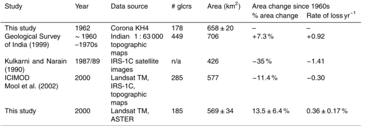
The study area encompasses glaciers in the eastern Himalaya (27◦04′52′′N to 28◦08′26′′N latitude and 88◦00′57′′E to 88◦55′50′′E longitude), located on either side of the border between Nepal and India in the Ganges and Brahmaputra basins (Fig. 1). Relief in this area ranges from 300 m to 8598 m (Mt. Kanchenjunga). Long valley

5

glaciers cover about 68 % of the glacierized area, mountain glaciers cover 28 %, and the remaining are cirque glaciers and aprons (Mool et al., 2002). The glacier ablation area is typically covered by heavy debris-cover originating from rockfall on the steep slopes (Mool et al., 2002), reaching up to a thickness of several meters at the glacier termini (Kayastha et al., 2000). The eastern part of this area constitutes the Sikkim

10

province of India, mapped in 1970 by Survey of India (Shanker, 2001; Sangewar and Shukla, 2009). The western part is located in eastern Nepal, and encompasses the Ta-mor and Arun basins. Climatically, this area of the Himalaya is dominated by the South Asian summer monsoon circulation system (Bhatt and Nakamura, 2005) caused by the inflow of moist air from the Bay of Bengal to the Indian subcontinent during the summer

15

(Yanai et al., 1992; Benn and Owen, 1998). The Himalaya and Tibetan plateau (HTP) acts as a barrier to the monsoon winds, bringing about 77 % of precipitation on the south slopes of the Himalaya during the summer months (May to September) (Fig. 2). This climatic particularity causes a “summer-accumulation” glacier regime type, with accumulation and ablation occurring simultaneously in the summer (Ageta and Higuchi,

20

1984). In Sikkim, rainfall amounts range from 500 to 5000 mm per year, with annual av-erages of 3580 mm recorded at Gangtok station (1812 m) (1951 to 1980) (IMD, 1980), and 164 rainy days per year (Nandy et al., 2006). Mean minimum and maximum daily temperatures at this station were reported as 11.3◦C and 19.8◦C, with an average of 15.5◦C based on the same observation record (IMD, 1980).

(6)

TCD

8, 3949–3998, 2014

from 1962 to 2006

Title Page

Tables Figures

◭ ◮

Back Close

Full Screen / Esc

Discussion

P

a

per

|

Discus

sion

P

a

per

|

Discussion

P

a

per

|

Discussion

P

a

per

|

3 Methodology

3.1 Data sources

3.1.1 Satellite imagery

Remote sensing datasets used in this study are summarized in Table 1, and included: (1) baseline remote sensing data for the 1960’s decade from Corona declassified

im-5

agery (year 1962); (2) “reference” datasets for 2000 decade from Landsat ETM+_and

ASTER and (3) 2006/09 high-resolution imagery from QB and WV, all described below. (1) Corona KH4 scenes (year 1962) were obtained from the US Geological Survey EROS Data Center (USGS-EROS 1996). The Corona KH4 system was equipped with two panoramic cameras (forward-looking and rear-looking with 30◦ separation angle),

10

and acquired imagery from February 1962 to December 1963 (Dashora et al., 2007). We chose images from the end of the ablation season (October/November in this part of the Himalaya), suitable for glaciologic purposes. Six Corona stripes were scanned at 7 microns by USGS from the original film strips. The nominal ground resolution re-ported for the KH4 mission is 7.62 m (Dashora et al., 2007); however, we calculated an

15

actual pixel size of approximately 2 m using the scale of the photos and the scan res-olution. Raw, unprocessed Corona images obtained from USGS are known to contain significant geometric distortions due cross-path panoramic scanning. Furthermore, the Frame Ephemeris Camera and Orbital Data (FECOD) camera/spacecraft parameters (roll, pitch, yaw, speed, altitude, azimuth, sun angle and film scanning rate) for Corona

20

missions, needed to construct a camera model and to correct these distortions are not available. Orthorectification of Corona scenes is notoriously diﬃ_{cult due to the heavy}

distortions, so here we describe in detail the methodology used.

We defined a non-metric camera model in ERDAS Leica Photogrammetric Suite (LPS), with parameters (focal length, air photo scale, flight altitude) extracted from the

25

(7)

TCD

8, 3949–3998, 2014

from 1962 to 2006

Title Page

Tables Figures

◭ ◮

Back Close

Full Screen / Esc

Discussion

P

a

per

|

Discus

sion

P

a

per

|

Discussion

P

a

per

|

Discussion

P

a

per

stripes simultaneously, and model parameters were calculated on the basis of 117 ground control points (GCPs) extracted from the panchromatic band of the 2000 Land-sat ETM+_{image (15 m spatial resolution). GCPs and were identified on the Landsat}

image on non-glacierized terrain including moraines, river crossings, and outwash ar-eas. Tie points (TPs) were digitized from one Corona strip to another as well as on the

5

Landsat image. Elevations were extracted from the Shuttle Radar Topography Mission (SRTM) DEM v.4 (CGIAR-CSI 2004) and were used to correct eﬀ_{ects of topographic}

terrain displacements. The Corona stripes were mosaicked in ERDAS LPS to produce the final orthorectified image. The horizontal accuracy (RMSEx,y) of the bundle block adjustment process was 10.5 m. An independent analysis of location accuracy using 30

10

check points chosen independently of the initial GCPs yielded an actual “ground” RM-SEx,y of the Corona images of∼60 m. This is consistent with accuracies obtained on

Corona images in Mexico, using a fitting software and the FECOD parameters (H. Sny-der, personal communication, 2011).

(2) The orthorectified Landsat ETM+_{scene from December 2000, obtained from the}

15

USGS Eros Data Center was used as “reference” dataset. The Landsat ETM+_scene

has seven spectral channels at 30 m spatial resolution, a thermal channel at 60 m and a panchromatic channel at 15 m, a revisit time of 16 days and a large swath width (185 km). In addition, six orthorectified ASTER scenes from 2000 to 2005 were ob-tained at no cost through the Global Land Ice Monitoring from Space (GLIMS) project

20

(Raup et al., 2007). The ASTER scenes have 3 channels in the visible wavelengths (15 m spatial resolution), 3 channels in the short-wave infrared at 30 m, and four ther-mal channels at 90 m, a swath width of 60 km and a revisit time of 16 days. Images were selected at the end of the ablation season for minimal snow, and had little or no clouds. The ASTER scenes were used to complement the Landsat-based glacier delineation

25

(8)

TCD

8, 3949–3998, 2014

from 1962 to 2006

Title Page

Tables Figures

◭ ◮

Back Close

Full Screen / Esc

Discussion

P

a

per

|

Discus

sion

P

a

per

|

Discussion

P

a

per

|

Discussion

P

a

per

|

Williams, 2012) and another ASTER scene from October 2002 was used to investigate surface temperature trends over debris covered tongues.

(3) Two QB scenes from January 2006 were obtained from Digital Globe as ortho-ready standard imagery (radiometrically calibrated and corrected for sensor and plat-form distortions) (Digital_Globe, 2007). These scenes cover an area of 1107 km2, and

5

were well-contrasted and mostly snow-free outside glaciers. We orthorectified these scenes in ERDAS Imagine Leica Photogrammetry Suite (LPS) using Rational Polyno-mial Coeﬃ_{cients (RPCs) provided by Digital Globe, using an SRTM DEM, and}

mo-saicked them in ERDAS Imagine. The scenes were resampled to 3 m-pixel size during the orthorectification process using the cubic convolution method to reduce disk space

10

and processing time. One WorldView-2 (WV2) panchromatic, ortho-ready scene at 50 cm spatial resolution from 2 December 2010 was also obtained to cover the terminus of Zemu glacier, which was missing from the QB extent. All datasets were registered to UTM projection zone 45N, with elevations referenced to WGS84 datum.

3.1.2 Elevation datasets

15

Two elevation datasets were used in this study: (1) the hydrologically-sound CGIAR SRTM DEM (90 m spatial resolution) (CGIAR-CSI 2004) was used to extract glacier parameters for the 2000 decade. The SRTM accuracy and biases have been quantified in several studies (Berthier et al., 2006; Fujita et al., 2008; Gardelle et al., 2012). Its vertical accuracy in our study area, calculated as root mean square (RMSEz) with

20

respect to 25 field-based GCPs was 31 m±10 m. The GCPs were obtained in the field

on non-glacierized terrain including roads and bare land outside the glaciers using a Trimble Geoexplorer XE series. (2) The Swiss topographic map (1 : 150 000 scale), compiled from Survey of India maps from the 1960s to 1970s, published by the Swiss Foundation for Alpine Research was used to extract 1960’s glacier elevation contours.

25

(9)

TCD

8, 3949–3998, 2014

from 1962 to 2006

Title Page

Tables Figures

◭ ◮

Back Close

Full Screen / Esc

Discussion

P

a

per

|

Discus

sion

P

a

per

|

Discussion

P

a

per

|

Discussion

P

a

per

3.2 Analysis extents

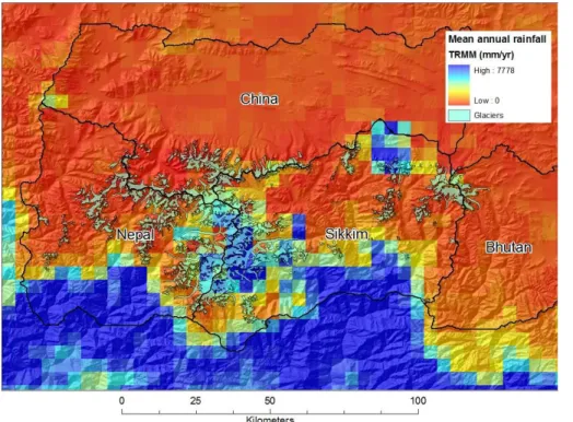
We defined two spatial domains for our study area (Fig. 1).Spatial domain 1includes the Sikkim province of India, eastern Nepal (Tamor and Arun basins), as well as parts of Bhutan and China (Table 2).

This spatial domain was split into four sub-regions on the basis of east-west and

5

north-south climate/topographic/political barriers, as shown in Fig. 3. Rainfall aver-ages from the Tropical Rainfall Measuring Mission (TRMM) data 2B31 product (Bhatt and Nakamura, 2005; Bookhagen and Burbank, 2006) are used to characterize the sub-regions climatically. The dataset contains rainfall estimates calibrated with ground-control stations derived from local and global gauge stations (Bookhagen and

Bur-10

bank, 2006) with a spatial resolution of 0.4◦, or ∼5 km. Given the well-known biases

in the TRMM data (Bookhagen and Burbank, 2006; Andermann et al., 2011; Palazzi et al., 2013), here we are not concerned with the absolute values of gridded precipita-tion, but only with characterizing the sub-regions in our study area using relative rainfall values. TRMM data integrated over 10 years (1998 to 2007) show diﬀ_{erences in}

pre-15

cipitation patterns among the four regions, and justifies our choice of spatial domains (Table 3). The eastern side of the study area (Sikkim) receives higher precipitation amounts than the western side (Nepal) (977 mm yr−1 versus 805 mm yr−1). There is a more pronounced north-south gradient in precipitation, with the lowest amount of precipitation on the China side (146 mm yr−1) (Table 3).

20

Spatial domain 2 is a subset of spatial domain 1, and comprises 50 glaciers from Nepal (Tamor basin) and Sikkim (Zemu basin), clean as well as and debris-covered. These glaciers were used for a more thorough analysis of glacier area and elevation changes and their dependence on climatic and topographic variables using correlations and multiple regression analysis for two time steps: the 1960’s decade (represented by

25

(10)

TCD

8, 3949–3998, 2014

from 1962 to 2006

Title Page

Tables Figures

◭ ◮

Back Close

Full Screen / Esc

Discussion

P

a

per

|

Discus

sion

P

a

per

|

Discussion

P

a

per

|

Discussion

P

a

per

|

3.3 Glacier delineation and analysis

For the 1960’s decade, glacier outlines were extracted from the panchromatic Corona imagery by thresholding the digital numbers (DN>200=_{snow/ice) based on visual}

interpretation. A 5×5 median filter was used to partially remove remaining noise, as

shown in other studies (Paul, 2007; Racoviteanu et al., 2008a). Manual corrections

5

were applied subsequently on the basis of the Swiss topographic map using on-screen digitizing in areas of poor contrast or transient snow/clouds, which obstructed the view of glaciers.

For the 2000’s Landsat/ASTER inventory, glaciers were delineated using the Nor-malized Diﬀ_{erence Snow Index (NDSI) (Hall et al., 1995), with a threshold of 0.7}

10

(NDSI>0.7=_{snow/ice). The NDSI algorithm relies on the high reflectivity of snow}

and ice in the visible to near infrared (VNIR) wavelengths (0.4–1.2 µm), compared to their low reflectivity in the shortwave infrared (SWIR, 1.4–2.5 µm) (Dozier, 1989; Rees, 2003). Compared to other band ratios (Landsat 3/4 and 3/5), the NDSI glacier map was cleaner and less noisy and was therefore preferred (Racoviteanu et al., 2008b).

15

A 5×5 median filter was used here as well to remove remaining noise, and a few

ar-eas were adjusted manually on the basis of the ASTER images, notably frozen lakes misclassified as snow/ice, and some glaciers underneath low clouds in the southern part of the image. Some transient snow persisting in the deep shadowed valleys was manually removed from the glacier outlines on the basis of the 1960’s topographic map.

20

Debris-covered glacier tongues were delineated using multispectral data (band ratios, surface kinetic temperature and texture) from the 27 November 2001 ASTER scene combined with and topographic variables in a decision tree, described in Racoviteanu and Williams (2012).

For the 2006/09 QB/WV2 images, ice masses were delineated using band ratios

25

3/4, then isodata clustering with a threshold of 1.07 (snow/ice>1.07), and a majority filter of 7×7 to remove noise. Debris-covered tongues for this dataset were delineated

(11)

TCD

8, 3949–3998, 2014

from 1962 to 2006

Title Page

Tables Figures

◭ ◮

Back Close

Full Screen / Esc

Discussion

P

a

per

|

Discus

sion

P

a

per

|

Discussion

P

a

per

|

Discussion

P

a

per

resolution images. We also mapped supraglacial lakes based on band ratios validated with texture analysis.

For all inventories in spatial domain 1, ice masses were separated into glaciers on the basis of the SRTM DEM, using hydrologic functions in an algorithm developed by Manley (2008), described in Racoviteanu et al. (2009). Glacier area, terminus elevation,

5

maximum elevation, median elevation, average slope angle and average aspect were extracted on a glacier-by-glacier basis using zonal functions. Average glacier thick-ness were calculated from mass turnover principles and ice flow mechanics Huss and Farinotti (2011), based on the approach of Farinotti (2009). Their method uses glacier outlines and the SRTM DEM to derive thickness estimates iteratively based on Glenn’s

10

flow law and a shape factor (Paterson, 1994). For simplicity and consistency for change analysis, we assumed no shift in the ice divides over the period of analysis, and ex-cluded all nunataks and snow-free steep rock walls from the glacier area calculations. Bodies of ice above the bergschrund were considered part of the glacier (Raup and Khalsa, 2007; Racoviteanu et al., 2009).

15

Glacier area changes (1962 to 2000) and their dependency on topographic and cli-matic variables were calculated on a glacier-by-glacier basis for the 50 glaciers in spa-tial domain 2. Elevation changes (1960 to 2000) were calculated for 21 debris-covered glacier tongues from 1960 to 2000 on the basis of the topographic map and the SRTM DEM. Elevation contours were digitized from the topographic map and were

interpo-20

lated using the TopoGrid algorithm in ArcGIS, using a 90 m pixel size. We then com-puted elevation diﬀ_{erences (1960–2000) over the debris covered tongues on a}

pixel-by-pixel basis and examined their spatial patterns. ASTER-based surface temperatures from the 2002 ASTER image were extracted for each debris-cover tongue, and the re-lationship between elevation diﬀ_{erences and surface temperature was evaluated along}

25

longitudinal transects on a pixel-by-pixel basis for the selected glaciers.

Uncertainties of glacier outlines derived using the semi-automated methods for Corona, Landsat/ASTER and Quickbird were ±3 %, ±6 and ±3 %, respectively.

(12)

TCD

8, 3949–3998, 2014

from 1962 to 2006

Title Page

Tables Figures

◭ ◮

Back Close

Full Screen / Esc

Discussion

P

a

per

|

Discus

sion

P

a

per

|

Discussion

P

a

per

|

Discussion

P

a

per

|

root mean square error (RMSE_z), using the accuracies of the SRTM DEM (±31 m) and

the error in the digitization of the topographic map (±25 m). Sources of uncertainty are

discussed in detail in Sect. 5.4.

4 Results

4.1 The Landsat/ASTER 2000 glacier patterns (Spatial domain 1)

5

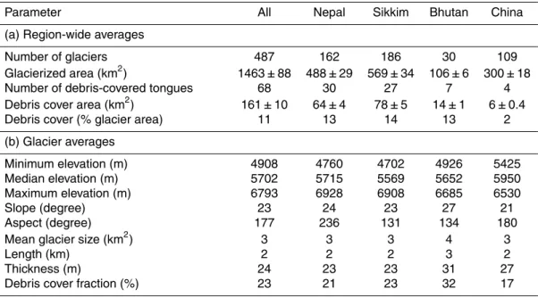
The 2000 glacier inventory based on Landsat and ASTER yielded 487 glaciers (of which 162 were situated in Nepal, 186 in Sikkim, 30 in Bhutan and 109 in China), covering an area of 1463 km2±88 km2(Table 4a). Of the total glacierized area in spatial

domain 1, a total of 160 km2±10 km2was covered by supraglacial debris (11 % of the

glacierized area). Of the 487 glaciers in this spatial domain, 68 glaciers (13 %) had

10

some percent of debris cover on their tongues. The debris cover distribution among the four regions in spatial domain 1 displays diﬀ_{erences in the north and south directions.}

In Sikkim, supraglacial debris covered an area of 78 km2±5 km2in 2000 (14 % of the

glacierized area), in contrast with the northern side of the Himalaya (China, 2 % of the glacierized area). The prevalence of debris cover on the south side of the Himalaya

15

can be explained in part by the geology and topographic patterns in the two regions. The northern side of the divide is part of the Tibetan plateau, situated in a monsoon shadow, with gentler slope and lower rates of erosion because of the dry climate. The southern slopes of the Himalaya are steep, comprise of soft sedimentary rocks and Precambrian crystalline rocks (Mool et al., 2002). These slopes are prone to erosion

20

and rock fall due to large amounts of moisture brought by the monsoon, which may explain the high amount of debris on the glacier surface on the south side of the divide. The behavior of debris covered vs. clean glaciers in relation to topographic/climatic patterns is explored in more detail in Sect. 4.3 below.

In 2000, glacier size ranged from 0.05–105 km2, with an average size of 3 km2 and

25

(13)

TCD

8, 3949–3998, 2014

from 1962 to 2006

Title Page

Tables Figures

◭ ◮

Back Close

Full Screen / Esc

Discussion

P

a

per

|

Discus

sion

P

a

per

|

Discussion

P

a

per

|

Discussion

P

a

per

about three times larger than tropical glaciers for example, where the average glacier size was∼1 km2(Racoviteanu et al., 2008a). The frequency histogram of glacier area

(Fig. 4a) is skewed to the right (skewness =_{8.4), showing that glaciers with area} _<

10 km2 are predominant, and glacier size decreases non-linearly. The long right-tail extremes represent only a few glaciers with an area >100 km2. The prevalence of

5

small glaciers is a pattern faily common in inventories which include small glaciers, as we noted in the Cordillera Blanca of Peru in a previous study (Racoviteanu et al., 2008a).

Glacier termini elevations in spatial domain 1 ranged from 3990 m to 5777 m, with an average of 4908 m; median glacier elevation ranged from 4515 m to 6388 m, with

10

a mean of 5702 m (Table 4b). Considering glacier median elevation as a coarse ap-proximation of glacier equilibrium line altitude (ELA), our results are in agreement with Benn and Owen (2005), who documented higher ELA’s on the northern slopes of the Himalaya (6000–6200 m) compared to ELA’s the southern slopes (4600–5600 m), due to drier climate in the former. In our study area, we note a slight east-west gradient in

15

glacier elevations, with higher glacier minimum and median elevations on the western side (Nepal) (+_{50 m) compared to the eastern side (Sikkim). This may be explained}

by the location of glaciers on the western side of the topographic divide, away from the monsoon. The north–south gradient in glacier elevations is stronger than the east– west, with glacier termini and median elevations much higher on northern side of the

20

divide (China) compared to the southern side (Nepal/Sikkim) (+_{700 m and} +_{400 m}

respectively). These diﬀ_{erences seem to be consistent with general air circulation}

pat-terns in the area, where the Asian summer monsoon brings large amounts of precipita-tion on the southern slopes of the Himalaya, favoring glacier growth at lower elevaprecipita-tions. In contrast, the upper reaches of the valleys and the Tibetan plateau have a drier

cli-25

mate due to the monsoon being blocked by the topographic barrier (Clift and Plumb, 2008), causing glaciers to be found at higher elevations.

(14)

TCD

8, 3949–3998, 2014

from 1962 to 2006

Title Page

Tables Figures

◭ ◮

Back Close

Full Screen / Esc

Discussion

P

a

per

|

Discus

sion

P

a

per

|

Discussion

P

a

per

|

Discussion

P

a

per

|

(p >0.05) (Table 4b). Glacier length ranged from 0.08 km to 23 km (Zemu glacier), with

an average of 2 km (Fig. 4c). Mool (2002) reported a length of 26 km for Zemu glacier in 1970’s, and the Geologic Survey of India (Sangewar and Shukla, 2009) reported 28 km for the same glacier based on 1970 topographic maps. This suggests a de-crease in length of ∼5 km in 30 years for this glacier. Glacier thickness ranged from

5

3 m to 144 m, with the highest frequency for thickness less than 30 m (Fig. 4d). The fre-quency distribution of both length and thickness were positively skewed with long tails, indicating the prevalence of short, shallow valley-type glaciers, respectively. Glacier aspect shows two predominant orientations of the glacier tongues: west-northwest (W-NW) and east-northeast (E-NE) (Fig. 5). Glaciers in Nepal had an average aspect of

10

237◦_{(SW), whereas glaciers of Sikkim for example had an average orientation of 131}◦

(SE). In a previous inventory, Mool et al. (2002) attributed the predominant orientation of glaciers (south, southwest, southeast and east) to the higher temperatures on the western slopes, which prevent glacier growth compared to the colder eastern slopes.

4.2 Glacier area changes 1962–2006 (spatial domain 2)

15

Out of the 487 glaciers in spatial domain 1, a sample of 50 glaciers from Tamor basin in Nepal and Zemu basin in Sikkim (spatial domain 2) were used for deriving area changes from 1962 (Corona imagery) to 2000 (Landsat/ASTER) and 2006 (Quickbird). To minimize uncertainties due to diﬀ_{erences in rock outcrops specific to each dataset,}

we used the same rock outcrops for each dataset. We obtained an area change of

20

−10.3 % (−0.24 % yr−1±0.08 % yr−1) from 1962 to 2006 for the 50 glaciers (Table 5),

with double the rates from 2000 to 2006 (−0.43 % yr−1±0.9 % yr−1) compared to the

previous period 1962 to 2000 (−0.20±0.16 % yr−1). Our rates of change are within the

range of those reported in other studies, if we consider the uncertainties in the change estimates. For example, for Sikkim, our study yielded an area loss of−88.9±5 km2, or

25

−13.5 % of the glacierized area (−0.36 % yr−1±0.17 %) for the last 38 years. In a recent

study, Basnett et al. (2013) reported a glacier area change of 0.16 % yr−1_{from 1989/90}

(15)

TCD

8, 3949–3998, 2014

from 1962 to 2006

Title Page

Tables Figures

◭ ◮

Back Close

Full Screen / Esc

Discussion

P

a

per

|

Discus

sion

P

a

per

|

Discussion

P

a

per

|

Discussion

P

a

per

lower than our estimate. The Basnett et al. rates are also lower than the ones reported elsewhere in the eastern Himalaya by Bolch et al. (2008a) (−0.25 % yr−1in the Khumbu

region of Nepal from 1962 to 2001), using similar methodology and data sources.

5 Discussion

5.1 Topographic factors controlling glacier area change

5

The area change results presented above (−0.36 % yr−1±0.17 % in the last four

de-caades) point to rates of retreat that are half the ones reported in other parts of the Himalaya. For example, an area change of −0.7 % yr−1 was reported by

Kulka-rni et al. (2007) for the western Himalaya and in other glacierized mountain ranges such as Alps (Kääb et al., 2002), the Tien Shan (Bolch, 2007) and the Peruvian Andes

10

(Racoviteanu et al., 2008a). We speculate that eastern Himalaya glaciers may be less sensitive to climatic changes given their location in a monsoon-influenced area, which may provide enough precipitation to high altitudes to maintain accumulation. Basnett et al. (2013) examined annual climate records from the Gangtok station (1812 m), and found that mean annual temperatures increased at a rate of 0.04◦C yr−1in the last four

15

decades, with most warming observed during the winter, and a slight, non-significant decreasing trend in precipitation. However, given the location of the station well below the glacier termini, these data are not conclusive.

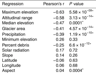
Correlations between topographic/climatic parameters and area change for the 50 glaciers in spatial domain 2 indicate that glacier maximum elevation, altitudinal range,

20

median elevation, glacier area, percent debris cover, aspect and precipitation were correlated with the percent area change from 1962 to 2006 (correlation statistically significant at the 90 % confidence interval,p <0.1) (Table 6). The strongest (negative) correlation with area change was found for maximum elevation and altitudinal range, indicating larger area changes for glaciers situated on lower summits, and with a small

25

(16)

ra-TCD

8, 3949–3998, 2014

from 1962 to 2006

Title Page

Tables Figures

◭ ◮

Back Close

Full Screen / Esc

Discussion

P

a

per

|

Discus

sion

P

a

per

|

Discussion

P

a

per

|

Discussion

P

a

per

|

diation and minimum elevations were not statistically significant, and they were only weakly correlated to area change (Table 6). On a glacier-by-glacier basis, glaciers lost

−0.7 % to−64 % of their area, with a mean of 25 % (−0.56 % yr−1) from 1962 to 2006

(Fig. 6). Spatial patterns of these area changes (Fig. 6) show largest area changes (>50 % area loss) for several glaciers in the northern and southern parts of the study

5

area. A closer look at these glaciers showed that they are small (<1 km2), steep (aver-age slope of 25◦), have little debris cover (<6 % of glacier area on average), and have termini elevations of 4423 to 5500 m.

Correlation analysis suggests a greater glacier area loss for south-facing slope aspects. Furthermore, smaller glaciers situated at lower maximum elevations, with

10

a smaller altitudinal range exhibited larger rates of area change. These results are con-sistent with observations from a diﬀ_{erent climatic area, the Cordillera Blanca of Peru}

(Racoviteanu et al., 2008a), indicating consistent patterns in glacier behavior. The rela-tionship between the debris cover percent of glacier area and area loss was statistically significant at 95 % confidence interval (p <0.05), i.e. glaciers with larger parts of their

15

area covered by debris experienced less area loss. This is to be expected given the potential insulating eﬀ_{ect of debris cover on glaciers above a certain “critical” debris}

thickness (Mihalcea et al., 2008; Zhang et al., 2011). There were diﬀ_{erences in area}

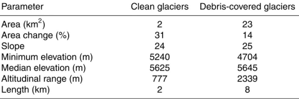
changes between clean and debris covered glaciers. Figure 7a and b shows a larger spread and a higher percentage of area loss of clean glaciers compared to

debris-20

covered glaciers. Between 1962 and 2006, clean glaciers lost 3.4 to 64 % of their area with a mean of 32.6 %, while debris-covered glaciers lost only 0.7 % to 61 % of their area, with a mean of 14.3 % on a glacier-by-glacier basis. The diﬀ_{erence in mean rates}

of area change between clean and debris covered glaciers was statistically significant based on two-sampleF test (pvalue<0.05).

25

Topographic parameters of debris-covered vs. clean glaciers may explain some of these diﬀ_{erences in area changes. Statistical analysis (two sample}_F _{test for variances)}

showed significant diﬀ_{erences between the debris-covered and clean glaciers}

(17)

TCD

8, 3949–3998, 2014

from 1962 to 2006

Title Page

Tables Figures

◭ ◮

Back Close

Full Screen / Esc

Discussion

P

a

per

|

Discus

sion

P

a

per

|

Discussion

P

a

per

|

Discussion

P

a

per

length (p <0.05) (Table 7). Clean glaciers in this area are∼10 times smaller (2 km2

on average) than debris-covered glaciers (23 km2), they have higher termini elevations (+_{535 m), and an elevation range about 3 times smaller than debris-covered glaciers}

(Table 7), which may all contribute to their higher rates of retreat.

In Figs. 8 and 9 we illustrate a few of these changes in more detail, using high

5

resolution Corona and QB imagery. Figure 8 a and b shows the rapid growth of the supra-glacier lake on S. Lonak glacier in Sikkim, also noted in Basnett et al. (2013). Glaciers on the upper northern part of the image are most likely rock glaciers, where some of the ice underneath has collapsed, but the area changes are less visible, and more uncertain, as pointed above. A closer look at a subset area (Fig. 9) shows two

10

adjacent glaciers (N. Lonak and S. Lonak) which underwent mass wasting. Their ter-minus retreated∼650 m to 1.3 km respectively from 1962 to 2006, with visible growth

of a supraglacial lake. Another branch of N. Lonak glacier has wasted significantly (∼1.5 km from 1962 to 2006), and a glacier outlet is now clearly visible. The terminus

of the glacier in 2006 is uncertain, since some part of the glacier terminus may be

in-15

active. In contrast, other debris-covered glaciers such as the near-by Jongsang glacier in the upper right part of the image does not show significant rates of terminus retreat (∼100 m in 44 years), in spite of increase in the area of supraglacial lakes.

5.2 Glacier elevation changes for debris-covered tongues 1960–2000

Given that some of the glaciers investigated here show little area change, the

ques-20

tion remains whether some of these glaciers are experiencing elevation changes (thin-ning/thickening), and what may govern these changes (for example, debris cover or supra glacial lakes). In this area, supraglacial lakes covered only 5.8 % of the area of the debris-covered tongues in 2006/09, as delineated from QB/WV2 imagery. Some of the glaciers, for example Zemu, the largest glacier in this area, had 27 % of its area

25

(18)

TCD

8, 3949–3998, 2014

from 1962 to 2006

Title Page

Tables Figures

◭ ◮

Back Close

Full Screen / Esc

Discussion

P

a

per

|

Discus

sion

P

a

per

|

Discussion

P

a

per

|

Discussion

P

a

per

|

glacierized area on a glacier by glacier basis). We chose these 21 glacier tongues to evaluate elevation diﬀ_{erences from 1960 to 2000 on a pixel-by-pixel basis (Fig. 10).}

We found that debris-covered tongues experienced an average lowering of−30.8±

39 m from 1960’s to 2000 (−0.8 m±0.9 m yr−1), which are similar to annual rates

re-ported in Gardelle et al. (2013) in the same climatic zone (Bhutan, −0.5±0.13 yr−1

5

and Hengdun Shan, −0.81±0.13 yr−1) for the period 2000–2011. Our rates are

lower than surface lowering in the ablation zones of glacier further west (Karakoram,

−0.33±0.16 yr−1) (Gardelle et al., 2013). We obtained higher thinning rates for glaciers

in contact with a growing pro-glacial lake, such as S. Lonak glacier discussed above (“A” in Fig. 10). Other glaciers such as Zemu (“B” on Fig. 10) display heterogeneity in

10

the elevation changes, with less distinct spatial patterns. In Fig. 10 we note larger eleva-tion diﬀ_{erences in the mid-upper zone of the ablation area of debris-covered tongues,}

and generally thickening towards the terminus, for example Yalung glacier (“C”) and Kanchenjunga glacier (“D”). The latter shows an interesting pattern of “bulging” of de-bris in the mid-lower part of the dede-bris-covered area, which we speculate might be due

15

to a thickening wave that is reaching the glacier terminus. Due to the lack of velocity or mass balance measurements in this area, we cannot assert this. Here we consider that high rates of thinning of >150 m, which are observed towards the rock walls in the upper, steep parts of the debris-covered area, are most likely due to errors in the topographic map in these areas.

20

5.3 Supraglacial surface temperature patterns

To explain some of these diﬀ_{erence in thinning/thickening patterns, we extracted}

sur-face temperature along longitudinal transect for a few glaciers, as shown in Fig. 10. Here we are presenting one of the glaciers, Zemu glacier (“B” in Fig. 10). Surface temperature patterns derived from 2002 ASTER imagery for Zemu glacier (Fig. 11)

25

display a large variability, particularly for the 10 km towards the glacier terminus. As a general trends, we note higher surface temperatures from the terminus to∼12 km

(19)

temper-TCD

8, 3949–3998, 2014

from 1962 to 2006

Title Page

Tables Figures

◭ ◮

Back Close

Full Screen / Esc

Discussion

P

a

per

|

Discus

sion

P

a

per

|

Discussion

P

a

per

|

Discussion

P

a

per

atures start decreasing from about 12 km from the glacier terminus to the limit with clean ice (middle of the ablation zone), indicating a thinner debris cover. Elevation dif-ferences display a high variability, with spikes of large changes in areas around supra-glacial lakes and ice cliﬀ_{s, which in general accelerate ablation (Sakai, 2002; Fujita and}

Sakai, 2014). In a diﬀ_{erent paper (Racoviteanu and Williams, 2012), we found similar}

5

patterns of surface temperature increasing towards the glacier terminus, indicating the presence of thicker supraglacial debris. On Fig. 11, the relationship between eleva-tion changes and surface temperature is more clear in the middle-upper debris area mentioned above, where we also note larger elevation diﬀ_{erences (thinning). There is}

less variability of surface temperature than the lower part, probably associated with

10

thin supra-glacial debris in this area. Regression analysis using surface temperature as explanatory variable for Zemu showed a non-significant dependency of elevation changes on surface temperature (p >0.05). An ordinary least-squared regression us-ing all 21 debris-covered tongues showed a weak dependency of elevation changes on surface temperature (R2=_{0.01). Standard residuals are close to normally distributed,}

15

with larger residuals in the upper part of the debris covered tongues (close to steep walls), discussed above.

5.4 Uncertainty estimates

Glacier outlines derived from remote sensing data, even when using well-established semi-automated methods, are known to be subject to various degrees of uncertainty,

20

as discussed in recent studies (Racoviteanu et al., 2009; Paul et al., 2013). This be-comes an important issue in glacier change analysis, where errors from various data sources accumulate at each processing step. In this study, we combined remote sens-ing data at various spatial and temporal resolutions with data from topographic maps and DEMs to derive glacier parameters and estimate of area/elevation changes. The

25

(20)

TCD

8, 3949–3998, 2014

from 1962 to 2006

Title Page

Tables Figures

◭ ◮

Back Close

Full Screen / Esc

Discussion

P

a

per

|

Discus

sion

P

a

per

|

Discussion

P

a

per

|

Discussion

P

a

per

|

due to the algorithms used for glacier mapping); (3) conceptual errors associated with the definition of a glacier, including mapping of ice divides, mixed pixels of snow and clouds, and internal rock all described in detail in Racoviteanu et al. (2009); (4) ele-vation errors due to inherent DEM uncertainty. Other types of errors, not discussed here, include errors due to atmospheric and topographic eﬀ_{ects, resampling, image}

5

co-registration, spectral mixing or raster to vector conversion. Instead, we focus on the main types of errors, with an emphasis on classification errors and conceptual errors, which we consider key for glacier area change estimates.

1. The orthorectification process of the 1962 Corona, using GCPs from a Landsat scene, yielded an error of ±10 m. Geolocation errors on the ground were

esti-10

mated using a trend analysis on the horizontal shifts between Corona and the reference Landsat scene, and resulted in ∼60 m, with the largest errors were

concentrated towards the edges of the images, mostly outside the glaciers. We consider that these errors minimally aﬀ_{ect our calculations of area change, since}

they do not impact the diﬀ_{erences in area. The geolocation accuracy of the}

stan-15

dard QB scenes is estimated as RMSE_x,_y of 14 m globally (Digital_Globe, 2007).

2. The accuracy of remote sensing glacier outlines is often estimated using the “Perkal epsilon band” around glacier outlines (Racoviteanu et al., 2009; Bolch et al., 2010), using a∼1-pixel variability (Congalton, 1991). Recent glacier

anal-ysis comparison experiments estimated the accuracy of automated glacier

out-20

lines using manually-derived outlines at multiple times and various analysts (Raup et al., 2007; Paul et al., 2013), and obtained a range of uncertainty of<5 % for re-mote sensing glacier outlines compared to high resolution imagery. In this study, we could not perform a validation using high-resolution imagery, since this was used as source imagery for area change. Instead, using the 1-pixel variability

25

(±30 m for Landsat/ASTER,±6 m for Corona and±3 m for QB outlines), we

(21)

TCD

8, 3949–3998, 2014

from 1962 to 2006

Title Page

Tables Figures

◭ ◮

Back Close

Full Screen / Esc

Discussion

P

a

per

|

Discus

sion

P

a

per

|

Discussion

P

a

per

|

Discussion

P

a

per

method is known to slightly over-estimate the errors described in Burrough and McDonnel (1998), so we consider our overlal area accuracy estimates to be rather conservative, and accommodate other errors not considered here (higher un-certainty of debris-covered tongues, GIS operations etc.). For manually-adjusted glacier outlines, including some of the debris-covered tongues, we minimized

er-5

rors by using screen digitizing in streaming mode, with a high density of vertices.

3. Conceptual errors are relevant here in the context of area change and relate to how the glaciers were defined. The glaciologic community has come to some consensus on how these rules should be applied (Racoviteanu et al., 2009), and here we comply to these guidelines. For consistency, we removed internal rocks

10

from all the area calculations; we manually removed perennial snowfields from the glaciers; we included “inactive” bodies of ice above the bergschrund as part of a glacier. Uncertainties in area change were computed as the RMSE of the uncertainties embedded in each dataset, from classification errors above, and amounted to 3–6 % of the glacierized area. Uncertainties related to diﬀ_erences

15

in internal rocks in each dataset were derived by comparing area changes com-puted with internal rocks specific to each dataset, vs. “merged” internal rocks from each datasets. The diﬀ_{erences in glacier datasets due to rock}

inconsisten-cies amounted to∼2 % glacier area, inducing diﬀerences in the rates of change in

area of±0.05 % yr−1. For simplicity, here we neglected the area change that might

20

be due to exposure of new internal rock due to glacier ice thinning. The glacier area changes computed from 1962 to 2006 suggest a higher rate of retreat in the last decade (−0.43 % yr−1±0.9 % from 2000 to 2006) compared to the previous

period (−0.20 % yr−1±0.16 % from 1962 to 2000). We speculate that some of this

apparent “accelerated” rate of glacier retreat in the last decade might be due to

25

the diﬀ_{erence in spatial resolution of the imagery. Due to the short time period}

(22)

TCD

8, 3949–3998, 2014

from 1962 to 2006

Title Page

Tables Figures

◭ ◮

Back Close

Full Screen / Esc

Discussion

P

a

per

|

Discus

sion

P

a

per

|

Discussion

P

a

per

|

Discussion

P

a

per

|

4. Elevation errorsin the glacier vertical changes were calculated using the RMSE_z, assuming an error of 25 m for the 1960’s topographic map (1/4 of the contour interval) and the calculated error for SRTM of 31 m, yielding an elevation change of 30.5 m±39 m. The errors associated with digitizing of the topographic map are

considered smaller than errors associated with the original map (Paul, 2003).

5

5.5 Comparison with other areas

Comparison of our results to other studies in this area of Himalaya is subject to incon-sistencies and inaccuracies in the classification methods used. For example, in Sikkim, our study estimated 569 km2±70 km2 of glacierized area for Sikkim in 2000 period

based on Landsat/ASTER data (Sect. 4.1). For the same time period, Mool et al. (2002)

10

reported 285 glaciers with an area of 577 km2 based on the same source imagery (Landsat ETM+_{) (Table 8). These two area estimates di}ﬀ_{er only by 8.2 km}2 _{(1.4 %) of}

our estimated area. The significant diﬀ_{erence in glacier numbers (186 glaciers in our}

study compared to 285 glaciers in ICIMOD study) are most likely due to the way in which ice masses were split and how glaciers were counted. Methodology diﬀ_erences

15

and inconsistencies in glacier estimates are quite common in multi-temporal image analysis performed by diﬀ_{erent analysts, and were previously noted in other areas of}

the world (Racoviteanu et al., 2009). Similarly, for the 1962 decade, our analysis of Corona 1962 imagery for Sikkim yielded 178 glaciers with an area of 658 km2±20 km2.

In a recent publication (Racoviteanu et al., 2014), we reported 158 glaciers with an

20

area of 742 km2 in 1960s based on the Swiss topographic map, which is 13 % higher than our new estimates based on Corona imagery from 1962. We consider the Corona estimates more reliable than the topographic map, and we use this dataset as the baseline for comparison with more recent imagery. Our 1962 Corona glacier inventory diﬀ_{ers by 48.3 km}2_{, or}_∼_{7 % from the inventory published by the Geological Survey of}

25

(23)

TCD

8, 3949–3998, 2014

from 1962 to 2006

Title Page

Tables Figures

◭ ◮

Back Close

Full Screen / Esc

Discussion

P

a

per

|

Discus

sion

P

a

per

|

Discussion

P

a

per

|

Discussion

P

a

per

persistent snow as glacial ice in the 1960’s–1970’s source aerial imagery. In contrast, another study (Kulkarni, 1992b), reported a glacierized area of 431 km2 for Sikkim in 1987/88 based on Indian IRS-1A and Landsat data. Compared to our Corona inventory, this would suggest an area loss of 42 % since the 1960’s–1970’s (2.1 % yr−1) followed by a subsequent glacier growth in the 2000s decade (based on our Landsat analysis).

5

We consider the 1987/89 estimates to be highly unreliable, given that there are no glacier surges that might induce an apparent “glacier growth”. Besides, the 1987/89 area estimate is smaller than the 2000 area estimated both by our study and by Mool et al. (2002). We speculate that these diﬀ_{erences may be due to omissions of some}

debris-covered tongues from the glacier maps.

10

6 Summary and conclusions

In this study we combined remote sensing data from various sensors to construct a new glacier inventory for the eastern Himalaya, and to quantify glacier area and elevation changes in the last four decades. We have constructed two updated glacier invento-ries for this part of the Himalaya, based on 1962 Corona and 2000 Landsat/ASTER

15

imagery, respectively. Spatial trends of glacier area and elevation changes in the last decades include:

– Larger percent of debris cover on glaciers on the southern slopes of the Hi-malaya (14 % of the glacierized area) compared to northern slopes (2 %), with supraglacial lakes constituting about 6 % of the debris covered area;

20

– Glacier area change amounts to −0.24 %±0.08 % yr−1 from the 1960’s to the

2006’s, with a higher rate of retreat in the last decade (−0.43 % yr−1±0.1 % from

2000 to 2006) compared to the previous period (−0.2 % yr−1±0.06 % from 1962

to 2000);

– Greater glacier area changes for small, steep glaciers with a smaller altitudinal

25

(24)

TCD

8, 3949–3998, 2014

from 1962 to 2006

Title Page

Tables Figures

◭ ◮

Back Close

Full Screen / Esc

Discussion

P

a

per

|

Discus

sion

P

a

per

|

Discussion

P

a

per

|

Discussion

P

a

per

|

a glacier’s headwater elevation, glacier area, debris cover, aspect and precipita-tion;

– Higher rates of retreat for clean glaciers (−34.6 %, or−0.7 % yr−1) on a

glacier-by-glacier basis, compared to debris-covered glacier-by-glaciers (−14.3 % or−0.3 yr−1) in the

last decades, as noted also in other studies elsewhere (Racoviteanu et al., 2008a;

5

Basnett et al., 2013);

– General trends of thinning of debris-covered tongues (−30.8 m±39 m) on

aver-age over the last four decades), with thickening towards the terminus for some glaciers, and rapid growth of pro-glacier lakes for others.

In this study we showed that in spite of intensive, time-consuming pre-processing steps

10

of the Corona imagery for high altitude rugged terrain, declassified imagery from the 1960’s has an important potential for glacier change detection in data-sparse areas of the Himalaya, as pointed in other studies (Narama et al., 2007; Bolch et al., 2008a). Further work would be needed on order to use Corona stereo imagery to investigate elevation changes. In this study, we did not use a DEM constructed from Corona

im-15

agery to investigate glacier elevation changes due to the time constraints and the lack of availability of a high-resolution DEM from the 2000’s. By contrast, topographic maps proved to be an important data source for computing elevation changes when georef-erenced and checked carefully. We also showed the potential of ASTER day surface temperature for investigating supraglacial features and as a proxy for glacier thickness.

20

There is a general tendency of thicker supra-glacier debris for most debris-covered tongues, as suggested by surface temperature trends, but the link between surface el-evation changes and surface temperature is not yet conclusive and requires additional investigation. The geospatial datasets and the topographic/climatic links developed in this study can be further to understand the behavior of Himalayan glaciers, such as

25

spatial patterns of glacier melt, and the contribution of glaciers to water resources.

(25)

TCD

8, 3949–3998, 2014

from 1962 to 2006

Title Page

Tables Figures

◭ ◮

Back Close

Full Screen / Esc

Discussion

P

a

per

|

Discus

sion

P

a

per

|

Discussion

P

a

per

|

Discussion

P

a

per

grant (NSF DDRI award BC 0728075), a CIRES research fellowship, and a graduate fellow-ship from CU-Boulder. A. Racoviteanu’s post-doctoral research was funded by Centre Na-tional d’Etudes Spatiales (CNES), France. Participation of M. Williams was supported by the NSF-funded Niwot Ridge Long-Term Ecological Research (LTER) program and the USAID Cooperative Agreement AID-OAA-A-11–00045. ASTER imagery was obtained through the 5

NASA-funded Global Land Ice Measurements from Space (GLIMS) project. We are grateful to Jonathan Taylor at University of California-Fullerton for facilitating access to high-resolution imagery through the NASA Appropriations Grant # NNA07CN68G.

References

Ageta, Y. and Higuchi, K.: Estimation of mass balance components of a summer-accumulation 10

type glacier in the Nepal Himalaya, Geogr. Ann. A, 66, 249–255, 1984.

Andermann, C., Bonnet, S., and Gloaguen, R.: Evaluation of precipitation data sets along the Himalayan front, Geochem. Geophy. Geosy., 12, Q07023, doi:10.1029/2011gc003513, 2011.

Bahuguna, I. M., Kulkarni, A. V., Arrawatia, M. L., and Shresta, D. G.: Glacier Atlas of Tista 15

Basin (Sikkim Himalaya), SAC/RESA/MWRGGLI/SN/16, Ahmedabad, India, 2001.

Bajracharya, S. R. and Shrestha, B. (Eds.): The Status of Glaciers in the Hindu-Kush Himalauan Region, International Centre for Integrated Mountain Development (ICIMOD), Kathmandu, Nepal, 127 pp., 2011.

Bajracharya, S. R., Mool, P. K., and Shresta, A.: Impact of Climate Change on Himalayan 20

Glaciers and Glacial Lakes, ICIMOD, Kathmandu, 2007.

Basnett, S., Kulkarni, A., and Bolch, T.: The influence of debris cover and glacial lakes on the recession of glaciers in Sikkim Himalaya, India, J. Glaciol., 59, 1035–1046, 2013.

Benn, D. I. and Owen, L. A.: The role of the Indian summer monsoon and the mid-latitude westerlies in Himalayan glaciation: review and speculative discussion, J. Geol. Soc. London, 25

155, 353–363, 1998.

(26)

TCD

8, 3949–3998, 2014

from 1962 to 2006

Title Page

Tables Figures

◭ ◮

Back Close

Full Screen / Esc

Discussion

P

a

per

|

Discus

sion

P

a

per

|

Discussion

P

a

per

|

Discussion

P

a

per

|

Berthier, E., Arnaud, Y., Vincent, C., and Remy, F.: Biases of SRTM in high-mountain areas: implications for the monitoring of glacier volume changes, Geophys. Res. Lett., 33, L08502, doi:10.1029/2006GL025862, 2006.

Berthier, E., Arnaud, Y., Kumar, R., Ahmad, S., Wagnon, P., and Chevallier, P.: Remote sensing estimates of glacier mass balances in the Himachal Pradesh (Western Himalaya, India), 5

Remote Sens. Environ., 108, 327–338, 2007.

Bhambri, R. and Bolch, T.: Glacier mapping: a review with special reference to the Indian Hi-malayas, Prog. Phys. Geog., 33, 672–702, 2009a.

Bhambri, R., Bolch, T., Chaujar, R. K., and Kulshreshth, S. C.: Glacier changes in the Garhwal Himalayas, India during the last 40 years based on remote sensing data, J. Glaciol., 54, 10

543–556, 2010.

Bhambri, R., Bolch, T., Chaujar, R. K., and Kulshreshtha, S. C.: Glacier changes in the Garhwal Himalaya, India, from 1968 to 2006 based on remote sensing, J. Glaciol., 57, 543–556, 2011. Bhatt, B. C. and Nakamura, K.: Charactieristics of Monsoon rainfall around the Himalayas

re-vealed by TRMM precipitation radar, Mon. Weather Rev., 133, 149–165, 2005. 15

Bolch, T.: Climate change and glacier retreat in northern Tien Shan (Kazakhstan/Kyrgyzstan) using remote sensing data, Global Planet. Change, 56, 1–12, 2007.

Bolch, T., Buchroithner, M. F., Pieczonka, T., and Kunert, A.: Planimetric and volumetric glacier changes in the Khumbu Himalaya since 1962 using Corona, Landsat TM and ASTER data, J. Glaciol., 54, 592–600, 2008a.

20

Bolch, T., Buchroithner, M. F., Peters, J., Baessler, M., and Bajracharya, S.: Identification of glacier motion and potentially dangerous glacial lakes in the Mt. Everest region/Nepal using spaceborne imagery, Nat. Hazards Earth Syst. Sci., 8, 1329–1340, doi:10.5194/nhess-8-1329-2008, 2008b.

Bolch, T., Menounos, B., and Wheate, R.: Landsat-based inventory of glaciers in western 25

Canada, 1985–2005, Remote Sens. Environ., 114, 127–137, 2010.

Bolch, T., Pieczonka, T., and Benn, D. I.: Multi-decadal mass loss of glaciers in the Everest area (Nepal Himalaya) derived from stereo imagery, The Cryosphere, 5, 349–358, doi:10.5194/tc-5-349-2011, 2011.

Bolch, T., Kulkarni, A., Kääb, A., Huggel, C., Paul, F., Cogley, J. G., Frey, H., Kargel, J. S., 30