www.ann-geophys.net/25/2175/2007/ © European Geosciences Union 2007
Annales
Geophysicae
Low-frequency ionospheric sounding with Narrow Bipolar Event
lightning radio emissions: regular variabilities and solar-X-ray
responses
A. R. Jacobson1, R. Holzworth1, E. Lay1, M. Heavner2, and D. A. Smith3
1Earth and Space Sciences, University of Washington, Seattle, WA, USA 2Physics Dept., University of Alaska Southeast, Juneau, AK, USA 3ISR Division, Los Alamos National Laboratory, Los Alamos, NM, USA
Received: 1 June 2007 – Revised: 10 August 2007 – Accepted: 28 September 2007 – Published: 6 November 2007
Abstract. We present refinements of a method of
iono-spheric D-region sounding that makes opportunistic use of powerful (109–1011W) broadband lightning radio emissions in the low-frequency (LF; 30–300 kHz) band. Such emis-sions are from “Narrow Bipolar Event” (NBE) lightning, and they are characterized by a narrow (10-µs), simple emis-sion waveform. These pulses can be used to perform time-delay reflectometry (or “sounding”) of the D-region under-side, at an effective LF radiated power exceeding by orders-of-magnitude that from man-made sounders. We use this op-portunistic sounder to retrieve instantaneous LF ionospheric-reflection height whenever a suitable lightning radio pulse from a located NBE is recorded. We show how to correct for three sources of “regular” variability, namely solar zenith angle, radio-propagation range, and radio-propagation az-imuth. The residual median magnitude of the noise in re-flection height, after applying the regression corrections for the three regular variabilities, is on the order of 1 km. This noise level allows us to retrieve the D-region-reflector-height variation with solar X-ray flux density for intensity levels at and above an M-1 flare. The instantaneous time response is limited by the occurrence rate of NBEs, and the noise level in the height determination is typically in the range±1 km.
Keywords. Ionosphere (Ionospheric disturbances;
Iono-spheric irregularities; Instruments and techniques)
1 Introduction and background
Structure and variability of the lower ionosphere (“D”-layer, altitude<90 km) are difficult to monitor, for two main rea-sons:
First, the low plasma frequency at D-layer heights necessi-tates use of LF (low-frequency; 30–300 kHz) or VLF
(very-Correspondence to:A. R. Jacobson
low-frequency; 3–30 kHz) techniques. For these frequencies, suitable radio-sounder antenna dimensions (on the order of the half-wavelength, orλ/2=5 km forf=30 kHz) cannot be realized in practice, so that one must make do with ineffi-cient, low-gain antennas.
Second, the D-layer’s high electron-neutral collision rate causes high signal loss in D-layer radio sounding, further worsening the signal-to-noise problem already implicit in the low-gain antennas.
A feasible alternative to wideband-pulse radio sounding of the D-layer is opportunistic reception of extremely pow-erful, narrow-band VLF transmissions that are transmitted for other purposes (see, e.g., Piggott et al., 1965, and ref-erences therein; Thomson and Clilverd, 2001; Thomson and Rodger, 2005). Thomson’s and his colleagues’ use of this ap-proach over long paths in the day-lit hemisphere has provided a remarkably accurate proxy for instantaneous solar X-ray flux density. Reception of extremely powerful, narrow-band VLF transmissions has served also in the study of local iono-spheric perturbations, e.g. “Sprites” (Dowden et al., 1996), D-region heating (Cho and Rycroft, 1998), and the optical signature of D-region heating, known as “elves” (Fukunishi et al., 1996).
al., 2006). The method uses averaging (over several serics) of the mean sferic spectrum, from which structural parameters of the D-layer can be retrieved.
Our present work is intended to be an extension of the general approach of Cummer and of Cheng, that is, using opportunistic reception of powerful lightning sferics. Our present work will depart from the earlier work in three re-spects: First, we will use the LF spectrum and a class of tem-porally narrow lightning strokes, for higher time resolution. Second, we will emphasize lightning-to-receiver paths that tend to be shorter (200–800 km), so that the ionospheric first-hop echo and the ground wave are both received, but are well time-resolved from each other. Third, by recording both the ground wave and the resolved ionospheric echo, we will at-tempt to retrieve D-layer structural parameters from a single sferic, potentially allowing us to track the time-development of fast perturbations.
A key goal of our present work is to develop a tech-nique suitable for diagnosis of local (100s of km horizontal), rapidly-varying (seconds to hours) ionospheric perturbations. Examples of such transient and local electron-density per-turbations include those caused by energetic-particle precip-itation (Bortnik et al., 2006) and by powerful lightning dis-charges’s radiated fields. Local (horizontal scale<1000 km) disturbances of these sorts have been inferred from long-range VLF-beacon-signal amplitude and phase perturbations in work pioneered by the Stanford group (see references in, e.g., Lev-Tov et al., 1995). Their work strongly suggests that a steep-incidence LF sounder operating underneath a local-ized disturbance would observe transient changes in D-layer reflection height. This motivates the present, preliminary ar-ticle, which characterizes the noise and variability in the op-portunistic LF sounding method.
2 Technical approach
2.1 General approach
Our technical approach is based on the recording of narrow LF signals from the unique lightning stroke known as an “NBE”, or Narrow Bipolar Event (Jacobson, 2003; Jacobson and Light, 2003; Smith et al., 1999). NBEs are received by LF recorders of the transient vertical electric field at ground level, e.g. LASA, or Los Alamos Sferic Array (Smith et al., 2002). The pertinent facts about NBEs for this article in-clude:
(a) The NBE main pulse is fast (∼10-µs width) and pow-erful (peak effective radiated power in range 109–1011W). This provides an opportunity for high-resolution time-delayed-reflectometry (TDR) from the ionosphere.
(b) NBEs are a common (but not ubiquitous) intracloud discharge in many electrified storms (Jacobson et al., 2007; Jacobson and Heavner, 2005; Suszcynsky and Heavner, 2003; Wiens et al., 2007). The incidence of NBEs has been
studied for storms both in Florida (Jacobson et al., 2007; Ja-cobson and Heavner, 2005; Suszcynsky and Heavner, 2003) and in the United States Great Plains (Wiens et al., 2007). NBEs do not appear to constitute a consistent proportion of total lightning in a storm. NBEs’ incidence is, instead, ex-tremely inconsistent, although there is a tendency to be most common in extremely intense thunderstorms (Wiens et al., 2007). Some storms have no observable NBEs, while other storms have as many as 20% NBE incidence. The pattern is extremely inconsistent (Jacobson et al., 2007; Jacobson and Heavner, 2005; Suszcynsky and Heavner, 2003; Wiens et al., 2007).
(c) Recording of the NBE ground wave, followed by both the ionospheric and the ground-then-ionospheric echoes, allows retrieval of the source and “ionospheric reflector” heights (Smith et al., 2004), for lightning-to-receiver ranges 200–800 km.
Using NBEs as a transmitter-of-opportunity for measuring reflective height of the D-layer, we will attempt to answer the following questions:
(a) What are the major sources of reflection-height vari-ability, and can this variability be determined and corrected? (b) Can the residual variabilities after correction be inter-preted in terms of solar-flare activity during the last solar maximum?
(c) What is the sensitivity of the method?
We will address these three questions within the constraint of a sharp-boundary (i.e., mirror-like) reflection model. This model obviously lacks the richness of information provided by the full-wave, diffuse-profile VLF model used in the works of Thomson et al., of Cummer, and of Cheng et al. They are able to estimate the ionospheric gradient length, while we cannot do so under the constraints of our sim-ple model. A future publication will apply a full-wave ionospheric-reflection model to our LF data recordings. 2.2 Reflection model and height retrieval
Typical LASA multi-station recordings of a single NBE near Florida are shown in Fig. 1. Each panel contains the recording from a different station (e.g., “ta”) at a dif-ferent range (e.g., 300 km) from the NBE location. The NBE location itself has been determined by time-difference of arrival (TDOA) by LASA (Smith et al., 2002). The time scale is zeroed for each station at that station’s trig-ger time. The two vertical dashed lines indicate the ex-pected echo-arrival times for, respectively, the ionospheric and the ground-then-ionospheric echoes, based on a model which assumes a discrete mirror at an ionospheric height
Hi=61.2 km, Hs=13.1 km (a) 20020818_14.20.46.064261; range= 300 ta
(b) 20020818_14.20.46.064261; range= 371 kw
(c) 20020818_14.20.46.064261; range= 431 gv
(d) 20020818_14.20.46.064261; range= 447 te
(e) 20020818_14.20.46.064261; range= 475 kc
-100 0 100 200
t (μs) relative to each station’s trigger
E (v/m) -2 0 2 4 6 8
E (v/m) -4 0 4 8
E (v/m) -2 0 2 4 6
E (v/m) -1 0 1 2 3
E (v/m) -1 0 1 2
Fig. 1.Five-station LASA recordings at 14:20:46.624 UT from 18
August 2002, of the vertical electric field versus time during arrival of signals from a Narrow Bipolar Event. The zero of the time axis is set individually for each station, at that station’s own trigger time.
The ground wave is neart=0. The bold portion of data in the second
panel is the subset of data identified as “groundwave” and then both delayed and filtered to estimate the ionospherically-reflected signal. The small electric-field features near the dashed lines are the echoes from the ionosphere and from the ground-ionosphere combination. The dashed lines indicate modeled arrival times using a single
iono-spheric height (Hi=61.2 km) and source height (Hs=13.1 km). See
text.
VLF experience (Wait and Spies, 1964)), isotropic conduc-tor. Inadequacies of the sharp-boundary reflection model cause some inaccuracy in retrievals ofHi but only small er-rors inHs, which is of primary interest for lightning research. In the present approach we will modify our retrieval of ionospheric height and source height in three key ways: Modification 1: We will let each qualifying station provide
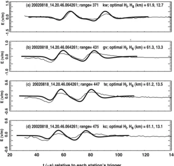
a separate retrieval for the two heights. It turns out that to the accuracy we presently seek in Hi, the dif-fuse (as opposed to sharp-boundary) ionospheric pro-file results in a systematic and monotone decrease of retrievedHi with range. We will continue to model a sharp-boundary, isotropic-medium reflection, but will let each range make its own estimate. We will then find an empirical regression ofHiwith respect to range, and correct allHi retrievals to “short” (200-km) range. Figure 2 shows a close-in view of the two echoes for the data in the second through fifth panels of Fig. 1. In each panel in Fig. 2, the light curve is the data for that station, while the heavy curve is a model of the data, based on a retrieval (see legend in each panel) for that station only.
v
20 40 60 80 100 120 140
t (μs) relative to each station’s trigger
(a) 20020818_14.20.46.064261; range= 371 kw; optimal Hi, Hs (km) = 61.9, 12.7
(b) 20020818_14.20.46.064261; range= 431 gv; optimal Hi, Hs (km) = 61.3, 13.3
(c) 20020818_14.20.46.064261; range= 447 te; optimal Hi, Hs (km) = 61.2, 13.5
(d) 20020818_14.20.46.064261; range= 475 kc; optimal Hi, Hs (km) = 61.1, 13.1 E (v/m) -1.5 0.0 1.5
E (v/m) -1.0 0.0 1.0
E (v/m) -0.6 0.0 0.6
E (v/m) -0.6 0.0 0.6
Fig. 2. Expanded view of ionospheric echoes from the more
dis-tant 4 stations in Fig. 1. The light curves are the various
sta-tions’ recorded data. The heavy curves are the modeled ionospheric echoes using a low-pass filter. Each modeled curve is individually
optimized by fitting its own optimumHi,Hs(see text). The range
and station designator are indicated near each station’s data and fit.
Modification 2: Our model imposes a fixed low-pass filter on the input (groundwave) waveform. Rather than gener-ate an echo model using a partially-conducting reflector (Smith et al., 2004), our present approach is to impose a frequency roll-off that is found to work better than the approach of Smith et al at mimicking the data, over the majority of events analyzed. By this, we mean that the modified approach results in a modeled ionospheric echo that more closely resembles the observed iono-spheric echo, relative to that of an echo model using a partially-conducting reflector (Smith et al., 2004). Each echo waveform in Fig. 2 is derived from the ground-wave ground-waveformEgndby a constant-phase filterF (f )in the frequency domain:
E(f )=Egnd(f )×F (f ) (1)
followed by return to the time domain and fi-nally imposition of a time delay for (first echo) the lightning-ionosphere-receiver path, or (second echo) the lightning-ground-ionosphere-receiver path. The filter is of the form
3 4 4
-10 -8 -6 -4 -2
log10 (X-ray flux density (W/m2))
hist(log
10
(X-ray flux
density)) w/ bin=0.1 0 2 4 6 8 X10
3 flare class C M X
Xs: 0.5 - 4.0 A Xl:1 - 8 A
0 50 100 150 solar zenith angle at ground (deg)
hist(zenith angle)
w/ bin=10 deg 0 2 4 6 8 X10
3
200 400 600 800 range (km)
hist(range) w/ bin=10 km 0.0 0.5 1.0 1.5 X10
4 (a)
(b)
(c)
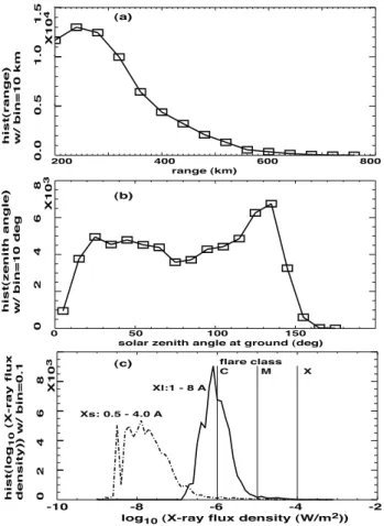
Fig. 3. Distributions of the 65 000 height retrievals against three
geophysical variables: (a) lightning-to-station range, (b) solar
zenith angle, and(c)both short- and long-wave solar X-ray flux
density. The X-ray data are 5-min-averaged SEM data from the GOES-10 satellite (see text).
LASA model (given by reflection off a conductor with conductivity 2.2X micro-mhos/m).
Modification 3: The standard LASA retrieval of heights (Smith et al., 2004) performs a correlation between the modeled and observed echo waveforms, to determine the “best” echo delays. In the present work, which seeks to minimize systematic errors inHi, we avoid correla-tion between two waveforms that are intrinsically some-what dissimilar, and instead compare derived peak times from the observations and from the model. Given the observed and modeled double echo, we search jointly inHi andHs to minimize the sum of the square of the residuals between modeled and observed peak times of the each of the two echoes. This requires some care, be-cause the data echo is corrupted by additive noise; see, e.g., the lower two traces (c and d) in Fig. 2. This noise makes it imperative not simply to identify the echo peak with the highest point in the noisy data, but rather to fit a smooth function to the echo and then find the peak of
the best-fit smooth function. For each echo peak, we fit the upper half of the echo with a fourth-order nomial, and we then find the peak of the best-fit poly-nomial. This results in an estimate of echo peak that is more robust against noise than would be the case if we simply found the raw echo data’s highest point. The modified height-determination method just described in-curs errors due to the imprecision of the fitted peak delay for the ionospheric echoes. As part of the automated calculation, we tabulate the estimated error in the peak location, based on the goodness of fit to the smooth polynomial model. Typical estimated errors in the fit are in the range 2–6µs. This causes reflection-height propagated errors in the range 0.5–1.5 km, due to uncertainties in the smooth-model fit.
2.3 Building a statistical database ofHi retrievals
We stored all LASA (Smith et al., 2002) NBE data from three years (2000, 2001, 2002) near the most recent solar maximum. This data was for the Florida subarray of LASA, centered on 28 deg N and−81.5 E. We restricted NBEs to those lying within 400 km from this array center. We then applied automatic height retrievals to all of those data, along the lines of Sect. 2.2 above. Several obvious quality fac-tors were then applied to select against noisy data or against echo waveforms that were poorly matched by the model. Af-ter this automated, criAf-teria-driven selection, we are left with 65 000 height retrievals, peaked in the year 2002, with fewer in 2001 and still fewer in 2000. (This year-to-year variation was wholly due to our reducing the trigger threshold as the system became more capable of handling greater volume of data; the year-to-year variation was not geophysical.) There are on average about two accepted height determinations per NBE, as opposed to the example in Fig. 2, which provides four height determinations.
3 Statistical results
3.1 Geophysical variabilities
0 50 100 150
solar zenith angle at ground (deg)
H
i
(km)
50 60 70 80 90 100
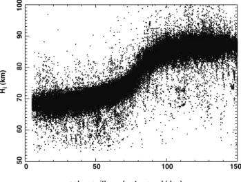
Fig. 4. Scatter plot of retrieved ionospheric height versus solar
zenith angle at ground, for all 65 000 height retrievals.
1999). On the other hand, for longer ranges than∼800 km, the ionospheric echo becomes poorly resolved (in time) from the ground-wave signal (Smith et al., 2004)). Together these two selection criteria contribute to the behavior of Fig. 3a.
Because data were gathered for several months each year (late Spring through early Fall), there is not a unique rela-tionship between local solar time and solar zenith angle. We shall see if zenith angle, without regard for day of year, can account for local-time variability in Hi. Figure 3b shows the distribution of zenith angle (at the ground). The obvi-ous control by zenith angle derives from the main source of ionospheric electron density, namely, photoionization by so-lar extreme ultra-violet radiation.
We use data from the National Oceanographic and Atmo-spheric Administration (NOAA) GOES-10 satellite on solar X-ray flux density, in 5-min averages. The X-ray flux density (W/m2)is monitored by GOES-10’s SEM payload both in a “longwave” channel (1–8µm) and in a “shortwave” channel (0.5–4.0µm), called Xl andXs, respectively. Each height retrieval is associated with a pairXlandXs from the 5-min period in which the NBE occurred. Figure 3c shows the dis-tribution of X-ray flux density tabulated for those 5-min pe-riods. Also shown are the conventional “C-flare”, “M-flare”, and “X-flare” thresholds for Xl.
3.2 Empirical correction for main variabilities inHi Figure 4 is a scatter-plot of the retrievedHi for all 65 000 height retrievals as a function of instantaneous solar zenith angle (at the ground). Obviously zenith angle accounts for the majority of natural variability ofHi. We define the min-imum range (200 km) as R0. In order to separate the Hi variability due to zenith angle, fromHi variability due to range, we take all the points in Fig. 4, select only those short-range retrievals within an arbitrarily selected short-range<250 km
0 50 100 150
solar zenith angle at ground (deg)
H
i
(km)
50 60 70 80 90 100
Fig. 5. Similar to Fig. 4, but for only those height retrievals from
short (200–250 km) range. The smooth curve is a parametric fit to the data (see text).
from the recording station, and fit the zenith dependence using only these short-range height retrievals “Hi0”.
Re-call that we do not perform any height retrievals for range
<200 km, so the bottom 50 km of range lies in the domain 200<range<250 km. This is shown in Fig. 5. The fit of
Hi0(Z) to zenith angle Z is shown as a line, and is based
on a model
Hi0(Z)=AXtanh[(Z−Zcent)/1Z] +1H (3)
where the best-fit parameters for amplitude, center, width, and offset are:
A=8.9 km,Zcent=78 deg,1Z=22 deg, and1H=79 km.
We can now apply the regression on Z to the ionospheric height, then use all the data together, regardless of zenith, to regress the range dependence of retrieved height. Let us define “scaled height” and “scaled range” as normalized by the best-fit ionospheric height at that solar zenith angle but at shortest range (200 km):
scaled height=Hi/Hi0(Z) (4a)
scaled range = range/Hi0(Z) (4b)
Figure 6 shows the scatterplot of scaled height versus scaled range. The decrease of scaled height with increasing range is due to the departure of the D-layer reflector from an ideal sharp boundary; it is, in reality, diffuse. As range increases, then so does angle of incidence, and thus the penetration of the radio wave into the medium decreases.
2 4 6 8 10 12
range / Hi0
H
i
/ H
i0
0.0 0.5 1.0 1.5
Fig. 6. Scatter plot of scaled height (that is, divided by the
mod-eled height at the appropriate zenith angle but at short range) versus scaled range, for all 65 000 height retrievals.
density tending to increase smoothly versus altitude in the range 70–90 km. This implies deeper penetration for LF radi-ation at smaller incidence angles, and shallower penetrradi-ation for grazing incidence (i.e., larger incidence angles). We cap-ture that trend via the sorting parameter of range, but it could equally be sorted via the parameter of angle-of-incidence.
We fit scaled height to a quadratic in scaled range; the 2nd-order-fit coefficient vector is:
(1.04,−0.014,5.6×10−5)
This best-fit ionospheric height will henceforth be called “Hi,fit”, and we will deal with a dimensionless height
(dif-ference) corrected for solar zenith angle and for range: dimensionless height=(Hi−Hi,fit)/Hi0(Z) (5)
This dimensionless height difference is plotted as a scatter-plot versus azimuth (deg clockwise from N, looking from the lightning location to the receiver) in Fig. 7. The reason for plotting the data versus azimuth is that the ionosphere is an anisotropic medium due to the geomagnetic field (Cummer, 1997; Cummer et al., 1998; Pitteway, 1965), and it is in prin-ciple possible that the observed reflection heights might have some systematic, detectable dependency on azimuth. Fig-ure 7 reveals a slight azimuth dependence, subtle compared to the dependencies on either zenith or range. Nonetheless we empirically fit the data in Fig. 7 to a function of the form
δ(dimensionless height)=AaXcos(az−az0) (6)
The best-fit amplitude and center are, respectively,Aa=0.012 andaz0=66 deg. The fit is shown in Fig. 7 as a solid curve.
From now on we include this correction δ(dimensionless height) into the dimensionless height (see Eq. 5).
(H
i
- H
i,fit
) / H
i0
-0.2 -0.1 0.0 0.1 0.2 -200 -100 0 100 200
azimuth CW from North (deg)
Fig. 7. Scatter-plot of dimensionless height corrected for zenith
and range (first differenced from range-controlled fit, then divided by the modeled height at the appropriate zenith angle but at short range) versus radio-propagation azimuth. The solid curve is a fit to a diurnal cosine, parametrized by amplitude and phase (see text).
The median absolute value of the final residual to the fit is about 0.015. That is, after removal of the “predictable” abilities due to zenith, range, and azimuth, the residual vari-ations in dimensionless height difference may be described by a median magnitude of 0.015, corresponding to ∼1 km unexplained median variability in daytime (whenHi0(Z=0) ∼70 km).
4 Contribution of solar-X-ray intensity to residual
height variability
4.1 Simple regression
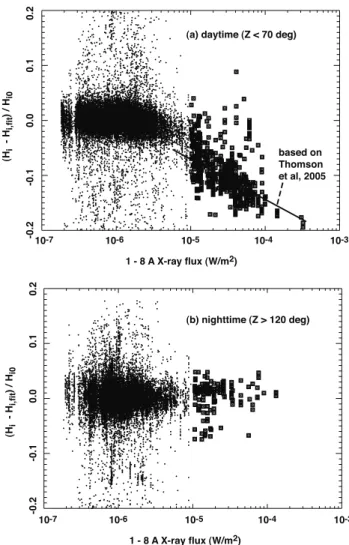
The 5-min-averaged GOES-10 long- and short-wavelength X-ray flux densities (see Fig. 3) will now be compared with their contemporaneous LASA height retrievals. Figure 8 shows scatter plots of dimensionless height difference (see Eq. 5) versus instantaneous long-wavelength X-ray flux den-sity, for daytime (Z<70 deg, Fig. 8a) and for nighttime
(Z>120 deg, Fig. 8b). The points where the X-ray flux
den-sity attains flare level “M” or “X” are marked with larger square symbols. Figure 8 excludes the dawn/dusk region
(70<Z<120 deg), because the D-region is in rapid
photo-chemical transition during dusk or dawn and may not be suitable to demonstrate a stationary height/X-ray-flux rela-tionship.
From Fig. 8 we observe:
effect correlated with solar X-rays, the effect could be only an indirect one, communicated to the nighttime hemisphere by magnetosperic substorm dynamics.
(b) Recently long-path VLF propagation phase has been shown to follow an exceptionally clear and reproducible pro-portionality to the logarithm of X-ray flux density (Thomson and Clilverd, 2001; Thomson and Rodger, 2005; Thomson et al., 2004). The main path studied was the Seattle (USA) to Dunedin (NZ) propagation of the 24.8 kHz radio beacon “NLK” transmitted near Seattle. During times when the path was sun-lit, the observed propagation phase and amplitude responses to solar-X-ray flux density were analyzed in terms of an exponential model of the ionospheric boundary, with two best-fit parameters: a heightHi and a logarithmic gra-dientβ. In the propagation model employed by Thomson and colleagues, the path attenuation is primarily influenced byβ, while the path phase is mainly influenced byHi. The sensitivity ofHi to the logarithm of long-wave X-ray flux density can be obtained by scaling from Fig. 11 in Thomson and Rodger (2005):
dHi/d(log10(Xl))= −5.1 km (7)
That result is for extremely long-range propagation (Seat-tle to Dunedin) at lower frequency (24.8 kHz) than our LF measurements. Nonetheless, let us compare our data to the scaling of Eq. (7). For a mean daytime, short-range height
Hi0(Z=0)of 70 km (see our Fig. 5 above), the scaling of
Thomson et al would imply that our dimensionless height difference (see Eq. 5 above) should vary with X-ray flux den-sity according to
d((Hi−Hi,fit)/Hi0(Z))/d(log10(Xl))= −0.073 (8)
at least on the high-flux tail where the radiative effects ex-ceed our system noise and other unexplained variabilities. This implied dependency is shown as the solid line in Fig. 8a. Remarkably, our daytime data, which is both noiser than the long-range VLF beacon method and involves a completely different approach to height retrieval, appears to be well de-scribed by the VLF (Thomson and Rodger, 2005) scaling.
Figure 9 shows similar scatter plots as does Fig. 8, but for the short-wave X-ray flux density. The symbol size is determined by long-wave X-ray level, but otherwise the ab-scissa value is for short-wave X-rays. Both Figs. 8 and 9 show dimensionless-height data only when the GOES X-ray-flux-density data is available. Occasionally the GOES data is indicated to be “bad” and is easily recognizable because in the archive it is pinned at a non-physical level. For example, the three low points near (1–2)×10−6(W/m2)in Fig. 9b are lacking in Fig. 8b. That is because theXlvalues are indicated to be “bad” in the NOAA archive.
4.2 Short-term clusters of data
Frequently a lightning storm in this Florida array area will last for up to a few hours without migrating more than about
(H
i
- H
i,fit
) / H
i0
-0.2 -0.1 0.0 0.1 0.2 10-7 10-6 10-5 10-4 10-3
1 - 8 A X-ray flux (W/m2)
10-7 10-6 10-5 10-4 10-3
1 - 8 A X-ray flux (W/m2)
(H
i
- H
i,fit
) / H
i0
-0.2 -0.1 0.0 0.1 0.2
(a) daytime (Z < 70 deg)
(b) nighttime (Z > 120 deg) based on Thomson et al, 2005
Fig. 8.Scatter plot of zenith-, range-, and azimuth-corrected
dimen-sionless height versus long-wave X-ray flux density, for(a)daytime,
and(b)nighttime. The heavy solid squares surround data at X-ray
fluxes greater than M-flare lower threshold.
50 km. This allows us to identify clusters of events from the same receiver station and from the same lightning storm. Us-ing such a cluster allows us to hold constant the observational geometry, and thus to monitor possible ionospheric height changes with minimal systematic variation. If the correc-tions for range and azimuth (see Sect. 3 above) were perfect, then there would be no added value in looking at clusters of data from the same storm and the same station. However, we do not believe that those corrections are such as to allow us to skip this prudent step.
(H
i
- H
i,fit
) / H
i0
-0.2 -0.1 0.0 0.1 0.2
(H
i
- H
i,fit
) / H
i0
-0.2 -0.1 0.0 0.1 0.2
10-9 10-8 10-7 10-6 10-5 10-6
0.5 - 4.0 A X-ray flux (W/m2)
10-9 10-8 10-7 10-6 10-5 10-6
0.5 - 4.0 A X-ray flux (W/m2)
(a) daytime (Z < 70 deg)
(b) nighttime (Z > 120 deg)
Fig. 9. Similar to Fig. 8, but plotted versus short-wave X-ray flux
density.
vectors (km Eastward, by km Northward) into square bins of 50-km×50-km size, and these in turn are spaced at 25-km intervals along both the East-West and North-South axes, for 50% overlap along each axis. We then iteratively search for the bin containing the most vectors. When we find that bin, we label its occupant height determinations as a new cluster of data. We then take those lightning events off the list of candidates for the next iteration, and repeat the pro-cess. The search is iterated until we can no longer find any 50-km×50-km bin containing at least 2 not-yet-used light-ning events vectors. At this point we have collected all the useable clusters of lightning storm/receiver vectors. Within each of the vector bins, the observing geometry is almost constant. Within each vector bin, we subtract the first re-trieval of dimensionless-Hi(see Eqs. 5 and 6 above) from all subsequent dimensionless-Hiretrievals within that bin, in or-der to null-out any residual bias from the cluster’s observing geometry. We refer to this product as “relative dimensionless height”.
19.5 20.0 20.5 21.0 21.5 22.0
UT hours on 20020726
1 - 8
A
X-ray flux (W/m
2)
10
-7 10 -6 10 -5 10 -4 10
-3
relative (H
i
- H
i,fit
) / H
i0
-0.4 0.0 0.4
zenith (deg) 0 20 40 60 80 (a)
(b)
(c)
Fig. 10.For a typical data cluster (see text), time series of(a)
long-wave X-ray flux density,(b)relative dimensionless height (see text),
and(c)solar zenith angle at ground. Each symbol is for the time of
a single height determination.
In this manner we find 13 257 clusters of data. Due to the temporal overlapping of the technique, this total count of clusters turns out to be about twice the number of truly independent storm/baseline combinations. In order not to miss vector clusters at the edge of regular time windows, we overlap the windows, and this results in a tendency toward double-counting.
Sometimes a data cluster’s time window includes part or all of a solar-flare X-ray transient. Figure 10 shows such a view of a flare, in this case an X-1 flare on 26 July 2002. The height determinations span about two hours and are irregu-larly spaced, due to the irregular occurrence of NBE light-ning events. Figure 10a shows the 5-min-averagedXl flux density from GOES-10 at the times of the lightning events. Figure 10b shows the relative dimensionless height, that is, the dimensionless height subtracted from the first less height in the cluster. Thus the first “relative” dimension-less height in the cluster is, by definition, zero. Figure 10c shows the solar zenith angle at the ground.
of the cluster’s first point. We then can plot all daytime cluster-relative dimensionless heights versus the correspond-ing cluster-relative X-ray flux densities, as in Fig. 11. Most of the clusters do not contain a dramatic X-ray transient, and this majority of points constitutes the ball of data near the ori-gin. In order to highlight cluster-relative X-ray flux-density magnitudes exceeding 0.5, we use a larger square symbol for those points. We perform a regression on only these high-lighted points; the best-fit slope is−0.079. This is to be compared with the slope of−0.073 implicit in Fig. 11 from Thomson and Rodger (2005). Our slope determination is cer-tainly much noisier than that of the earlier long-path VLF work, as is expected from a localized measurement such as steep-incidence sounding. Nonetheless we find it noteworthy that the LASA statistical regression of LF, steep-incidence height sensitivity to X-ray flux density agrees so well with the more precise regression from long-path VLF.
5 Discussion
As mentioned in Sect. 2.1 above, we posed three questions to be answered in this article. The next three subsections deal in sequence with those questions.
5.1 Major sources of regular reflection-height variability, and their correction
By “regular” variability, we mean a variability of the re-flection height straightforwardly related to, and predictable by, “independent” geophysical parameters. Of these regu-lar variabilities in reflection height, we find the most signif-icant to be due to solar zenith angle. Over several months, the D-layer insolation (at a set local time) is not constant, and zenith angle- which alone determines the insolation ge-ometry -is preferable to local time as a proxy for insolation. The next most significant regular variability is controlled by lightning-to-receiver range. Finally, the weakest regular vari-ability is controlled by the propagation azimuth. All three of these regular variabilities are appropriately best-fit and then corrected in the data. We combine all corrected data in a “di-mensionless height” that is scaled by the best-fit short-range height for the particular solar zenith angle.
5.2 Residual variabilities and solar-flare transients
We find that the response of dimensionless height to solar X-ray flux-density transients is noisy but consistent with the far less noisy predictions based on long-range VLF propagation in the Earth-ionosphere waveguide (Thomson and Rodger, 2005; Thomson et al., 2004).
5.3 Implications for the sensitivity of the method
After correction for the “regular” variabilities, and for vari-ability controlled by solar X-ray intensity, we are left with a
Fig. 11. Scatter plot showing dimensionless height for all heights
in all clusters (after subtracting the dimensionless height of the first point in each cluster), versus the logarithm of the long-wave X-ray flux density relative to the first point in each cluster. Points whose logarithm of the flux density differs from its cluster’s first point’s
flux density by more than±0.5 are marked by square symbols (see
text).
residual median dimensionless-height variability of around 0.015. For a mean daytime short-range height of 70 km, this implies a residual median noise magnitude of ∼1 km. This is on the order implied by the estimated statistical er-rors from the smooth-polynomial fit to the echo peak delay (see Sect. 2.2): The range of statistical errors propagates to a height error of 0.5–1.5 km.
We were able to estimate the sensitivity in daytime be-cause of the availability of solar-flares as a calibration source. During nightime, we do not have such a well-established and hemispherically homogeneous calibration source. However, we suspect that the nighttime sensitivity should be no worse, and possibly better than, the daytime sensitivity, due to a sim-ple propagation effect: During nighttime, the LF propagation is less lossy, and the ionospheric reflection coefficient is en-hanced (Pitteway, 1965) relative to daylit condition. This is the same reason why short-range VLF studies of ionospheric transients have been conducted during nighttime (Cheng and Cummer, 2005; Cheng et al., 2006).
Acknowledgements. We benefited from useful discussions with S. A. Cummer. K. Wiens has been of constant assistance with cer-tain complexities of the LASA archive. LASA was operated by Los Alamos National Laboratory during 2000–2002 under the auspices of the United States Department of Energy.
References
Bortnik, J., Inan, U. S., and Bell, T. F.: Temporal signatures of radi-ation belt electron precipitradi-ation induced by lightning-generated MR whistler waves: 2. Global Signatures, J. Geophys. Res., 111, A02205, doi:10.1029/2005JA011398, 2006.
Bortnik, J., Inan, U. S., and Bell, T. F.: Temporal signatures of radi-ation belt electron precipitradi-ation induced by lightning-generated MR whistler waves: 1. Methodology, J. Geophys. Res., 111, A02204, doi:10.1029/2005JA011182, 2006.
Cheng, Z. and Cummer, S. A.: Broadband VLF measurements of lightning-induced ionospheric perturbations, Geophys. Res. Lett., 32, L08804, doi:10.1029/2004GL022187, 2005.
Cheng, Z., Cummer, S. A., Baker, D. N., and Kanekal, S.
G.: Nighttime D region electron density profiles and
vari-abilities inferred from broadband measurements using VLF ra-dio emissions from lightning, J. Geophys. Res., 111, A05302, doi:10.1029/2005JA011308, 2006.
Cho, M. and Rycroft, M. J.: Computer simulation of the electric field structure and optical emission from cloud-top to the iono-sphere, J. Atmos. Solar-Terr. Phys., 60, 871–888, 1998. Cummer, S. A., Inan, U. S., and Bell, T. F.: Ionospheric D region
remote sensing using VLF radio atmospherics, Radio Sci., 33, 1781–1792, 1998.
Dowden, R. L., Brundell, J., Lyons, W. A., and Nelson, T.: Detec-tion and locaDetec-tion of red sprites by VLF scattering of subiono-spheric transmissions, Geophys. Res. Lett., 23, 1737–1740, 1996.
Fukunishi, H., Takahashi, Y., Kubota, M., and Sakanoi, K.: Elves: Lightning-induced transient luminous events in the lower iono-sphere, Geophys. Res. Lett., 23, 2157–2160, 1996.
Jacobson, A. R.: How do the strongest radio pulses from thunder-storms relate to lightning flashes?, J. Geophys. Res., 108, 4778, doi:10.1029/2003JD003936, 2003.
Jacobson, A. R. and Light, T. E. L.: Bimodal radiofrequency pulse distribution of intracloud-lightning signals recorded
by the FORTE satellite, J. Geophys. Res., 108, 4266,
doi:10.1029/2002JD002613, 2003.
Jacobson, A. R. and Heavner, M. J.: Comparison of Narrow Bipolar Events with ordinary lightning as proxies for severe convection, Mon. Weather Rev., 133, 1144–1154, 2005.
Jacobson, A. R., Boeck, W., and Jeffery, C.: Comparison of Nar-row Bipolar Events with ordinary lightning as proxies for the microwave-radiometry ice-scattering signature, Mon. Weather Rev., 135, 1354–1363, 2007.
Lev-Tov, S. J., Inan, U. S., and Bell, T. F.: Altutude profiles of localized D region density disturbances produced in lightning-induced electron precipitation events, J. Geophys. Res., 100, 21 375–21 383, 1995.
Piggott, W. R., Pitteway, M. L. V., and Thrane, E. V.: The numer-ical calculation of wave-fields, reflexion coefficients and polar-izations for long radio waves in the lower ionosphere. II, Phil. Trans. Roy. Soc. Lon., 257, 243–271, 1965.
Pitteway, M. L. V.: The numerical calculation of wave-fields, re-flexion coefficients and polarizations for long radio waves in the lower ionosphere. I, Phil. Trans. Roy. Soc. Lon., 257, 219–241, 1965.
Smith, D. A., Shao, X. M., Holden, D. N., Rhodes, C. T., Brook, M., Krehbiel, P. R., Stanley, M., Rison, W., and Thomas, R. J.: A distinct class of isolated intracloud lightning discharges and their associated radio emissions, J. Geophys. Res., 104, 4189–4212, 1999.
Smith, D. A., Eack, K. B., Harlin, J., Heavner, M. J., Ja-cobson, A. R., Massey, R. S., Shao, X. M., and Wiens, K. C.: The Los Alamos Sferic Array: A research tool for lightning investigations, J. Geophys. Res., 107(D13), 4183, doi:10.1029/2001JD000502, 2002.
Smith, D. A., Heavner, M. J., Jacobson, A. R., Shao, X. M., Massey, R. S., Sheldon, R. J., and Wiens, K. C.: A method for determining intracloud lightning and ionospheric heights from VLF/LF electric field records, Radio Sci., 39, RS1010, doi:10.1029/2002RS002790, 2004.
Suszcynsky, D. M. and Heavner, M. J.: Narrow Bipolar Events as indicators of thunderstorm convective strength, Geophys. Res. Lett., 30, 1879, doi:10.1029/2003GL017834, 2003.
Thomson, N. R. and Clilverd, M. A.: Solar flare induced iono-spheric D-region enhancements from VLF amplitude observa-tions, J. Atmos. Solar-Terr. Phys., 63, 1729–1737, 2001. Thomson, N. R., Rodger, C. J., and Dowden, R. L.: Ionosphere
gives size of greatest solar flare, Geophys. Res. Lett., 31, L06803, doi:10.1029/2003GL017345, 2004.
Thomson, N. R. and Rodger, C. J.: Large solar flares and their iono-spheric D region enhancements, J. Geophys. Res., 110, A06306, doi:10.1029/2005JA011008, 2005.