BANKING RETAIL CONSUMER FINANCE DATA GENERATOR – CREDIT SCORING DATA REPOSITORY

(1)

BANKING RETAIL CONSUMER FINANCE

DATA GENERATOR – CREDIT SCORING

DATA REPOSITORY

Karol Przanowski

*

Introduction

Currently predictive models and especially credit scoring models are very popular in the management of banking processes (Huang, 2007). It is generally the case that risk scorecards are used in credit acceptance processes to optimize and control any risk. Various forms of behavioral scorecards are also used for the management of repeat business (cross-up sell) and also for PD (probability of default) models in Basel RWA (Risk Weighted Assets) calculation (BIS-BASEL, 2005). It is oten suicient to obtain a list of about 10 account or client characteristics which, when combined, can predict their future behavior, their style of payments and their delinquency.

One may add that trivial fact scorecards are still of use and their methodology is well known, but on the other hand credit scoring can be still developed further and new techniques should always be tested. he main problem today is that there is no deined general testing ideology for new methods and techniques; there is no proven method to gauge their correctness. Many good articles are prepared based

on one particular case study, on one example of real data coming from either one or more than one bank (Malik and homas, 2009), (Huang and Scott, 2007) and (Majer, 2010). From a theoretical point of view, even if good results are reached and sound arguments put forward to suggest choosing one method instead of another, these results are usually reached using that particular data which indicate the diference, but other data will oten suggest a diferent conclusion; nobody can guarantee correctness for all cases. Other important reasons remain for why real banking data are not available globally and why they cannot be used by every analyst, namely reasons such as: legal constraints or new products with too short a data history. hese two factors lead us to search for a quite new approach for predictive modeling testing in banking usage.

It seems a sensible idea to start developing two parallel ways: real data and random-simulated data approaches. Even if the latter cannot replace real data, it can be very useful to understand better the relations among various factors in data; to imagine Abstract This paper presents two cases of random banking data generators based on migration matrices and

scoring rules. The banking data generator is a breakthrough in researches aimed at inding a method to compare various credit scoring techniques. These data are very useful for various analyses to understand the complexity of banking processes in a better way and are also of use for students and their researches. Another application can be in the case of small samples, e.g. when historical data are too fresh or are connected with the processing of a small number of exposures. In these cases a data generator can extend a sample to an adequate size for advanced analysis. The inluence of one cyclic macro-economic variable on client characteristics and their stability over time is analyzed. Some stimulating conclusions for crisis behavior are presented, namely that if a crisis is impacted by both factors: application and behavioral, then it is very diicult to clearly indicate these factors in a typical scoring analysis and the crisis becomes widespread in every kind of risk report.

Received: 27.11.2012 Accepted: 19.03.2013

JEL Classiication: C53

Keywords: credit scoring, crisis analysis, banking data generator, retail portfolio, scorecard building, predictive modeling

the complexity of the process and it can be an attempt to create a more general class of semi-real data. Let us consider some of the advantages of random data:

1) Today many analysts are trying to understand and to analyze the most recent crisis (Mays, 2009), among other things they are developing methods of indicating risk stability in sub-portfolios that remain stable over time. his is not an easy topic and it cannot be solved by typical predictive models based on target variables as in the case of a default risk. he notion of stability cannot be deined for every particular account or client. It is diicult to state that an account is stable, only the set of accounts can be tested, so this technique should be developed by a quite diferent method than a typical predictive modeling with a target variable. It can be formulated by the simple conclusion: the more accounts, the more robust the stability testing. Various scenarios based on the random data generator can be tested to see and to understand the problem better.

2) Scoring Challenges or Scoring Games. From time to time diferent competitions are organized by various institutions: banks, universities, consultancy companies or associations; to ind good modellers, or to test new techniques. Sometimes, data are used that have too many „real cases”. Here „too real” is understood as meaning that some real processes are unpredictable, because they are inluenced by many immeasurable factors. Even if scoring models are used in practice in these cases, it is not a good idea to use that data for competition. he best solution and the best choice is to use a random data generator directly predictable process.

3) Reject inference area (Huang and Scott, 2007). his topic requires further development. Random data can also be generated in practice for testing rejected cases, so it can be used for a better estimation of risk on a missed area and in order to gain experience.

4) Today there are two or more techniques of scorecard building (Siddiqi, 2005). We need to make some comparisons and carry out an analysis to deine recommendations: it must be clear when to use one method rather than another. he same situation can be applied for diferent variable selection methods.

5) Data extending. Sometimes collected data are too small, have too few defaults, or too brief length of history. Some properties can be studied and discovered but typical credit scoring techniques cannot be applied. In that case real data can be improved by adding some random rows gaining the possibility of making a deeply scoring analysis. Even though the new sample does not represent only real cases, its results can be of use as they can be used to produce variable conidence limits. To guarantee better prediction more than one scenario of random generator can also be considered.

6) Product proitability, bad debts and cut-ofs. For random data all these notions can be tested and analysts’ experience can be broadened.

7) Random data can also be a very important factor in the topic of data standardization or the idea of auditing. Let us imagine that the sotware tools for MIS (Management Information Systems) and KPI (Key Performance Indicators), reporting on the generic data structure, which has irstly been uploaded by random data, are already running. hen the auditing of any other data will be minimized only by the upload data process.

Simulation data are used in many areas, for example it is of use in the research of a telecommunication network by a system like OPNET . Some simulated data in the banking area by (Supramaniam and Shanmugam, 2009) and (Watson, 1981) are also developed.

he simplest retail consumer inance portfolio is the ixed installment loan portfolio. Here the process can be simpliied by the following assumptions:

1) for all accounts one due date in the middle of the month is deined (every 15th),

2) every client has only one loan,

3) a client can pay the whole installment, a few installments or pay nothing. hese can be categorized as either payment or non payment,

4) there are measured delinquencies on states: at the end of the month by indicating the number of due installments,

5) all customer and account properties are randomly generated by deined proper random distributions,

6) if the number of due installments reaches 7 (180 past due days) the process is stopped and an account is given a bad account status; any further collection steps are omitted,

7) if the number of paid installments reaches the total number of all installments then the process is stopped and an account is given a closed account status,

8) payments or missing payments are determined by three factors: the score calculated on account characteristics, migration matrix and adjustment of that matrix by one macro-economic variable time cycle,

9) a score is calculated separately for every due installments group. In more general cases a diferent score for every status can be deined: due installments 0, 1, ..., and 6.

(2)

present crisis was not predicted in time, it could at least have been indicated promptly. It seems that the best tool of risk control is migration matrix reporting. he goal of this paper can also be formulated in the following way: to create random data with the aim of obtaining the same results as those observed in reality using typical reporting like migration matrix, low-rates or roll-low-rates and vintage or default low-rates.

Detailed description of a data

generator

The main options

All data are generated from the starting date

T

e to

ending

T

_e_.

he migration matrix

M

_ij (transition matrix) is deined as a percent of one month transition from due installments

i

to due installments

j

. here is only one macro-economic variable dependent on the time described by the formula:

E m

_{( )}

_,where

m

is the number of months from

T

s. It should fulill

the following simple condition:

0 01

.

<

E m

( )

<

0 9

.

, because it is used as an adjustment of the migration matrix, so it has an inluence on the risk; in some months it produces a slightly greater risk and in some months a lower one.

Production dataset

he irst dataset contains all applications with all available customer characteristics and credit properties.

Customer characteristics (application data): 1) Birthday -

T

_Birth_{- with the distribution}

D

_Birth

2) Income -

x

Income a

-

D

_Income 3) Spending -

x

Spending

a

-

D

Spending

4) Four nominal characteristics -

x

Nom

x

a

Nom a

1

,...,

4 -

D

Nom₁

,

D

Nom₂

,...,

D

Nom₄, in practice they can

represent variables such as: job category, marital status, home status, education level, or others. 5) Four interval characteristics -

x

Int

x

a

Int a

1

,...,

4 -

D

Int Int Int

1

,

2

,...,

4, represent variables such as: job seniority, personal account seniority, number of households, household spending or others.

Credit properties (loan data):

1) Installment amount -

x

Inst

l

- with the distribution

D

_Inst 2) Number of installments -

x

N

l

inst -

D

Ninst

3) Loan amount -

x

Amount

x

l Inst l N l inst

=

⋅

4) Date of application (year, month) -

T

app 5) Id of application.

he number of rows per month is generated based on the distribution

D

Applications.

Transaction dataset

Every row contains the following information (transaction data):

1) Id of application.

2) Date of application (year, month) –

T

app 3) Current month -

T

cur

4) Number of due installments (number of missing payments) -

x

n

t

due

5) Number of paid installments -

x

n t

paid 6) Status -

x

status

t

- Active (A) - remains unpaid, Closed (C) - is paid, or Bad (B) - when

x

n

t

due

=

7

7) Pay days -

x

days t

- number of days from the interval

[

−15 15

,

]

before or ater due date in a current month when payment was made, if there is a missing payment, then pay days equal to missing value. Inserting the Production dataset into the Transaction dataset

Every month of the Production dataset updates the Transaction dataset with the following formulas: Tcur Tapp xn x x A x

t n t status t days t due paid

= , =0, =0, = , =0.

his is the process of inserting the starting points of new accounts.

Analytical Base Table - ABT dataset

he history of payments for every account is dependent on behavioral data, or, in other words, on the behavior of previous payments. his is, of course, the assumption of the data generator.

here are many theories on how to create behavioral characteristics. Here some simple methods to consider their last available time stamps (actual states) and to indicate their evaluations over time are presented. All data are prepared in ABT datasets, the

notion of Analytical Base Table (ABT) is used by SAS Credit Scoring Solution .

Let us set the current date

T

cur as a ixed value. he

actual states are calculated for that date by the formulas (actual data):

x

days act days t

=

+15,

x

_nact

x

n

t

paid

=

paid

,

x

n act

n t

due

=

due

,

x

_utlact

x

_nt

x

_Nl paid inst

=

/

,

x

dueutl

x

act n t N l due inst

=

/

,

x

_{years T}

_T

age act

Birth cur

=

(

,

),

x

_capacityact

=

(

x

_Instl

+

x

_Spendinga

) /

x

_Incomea

,

x

dueinc

x

act n t Inst l Income a due

=

(

⋅

) /

,

x

loaninc

x

act Amount l Income a

=

/

,

x

_seniorityact

=

T

_cur

−

T

_app

+

1,

where

years

()

calculates the diference between two dates in years.

Let us consider two time series of pay days and due installments for the last 11 months from a ixed current date by the formulas:

x

_daysact

( )

m

=

x

_daysact

(

T

_cur

−

m

)

,

x

n

m

x

T

m

act

n

act cur

due

( )

=

due

(

−

)

,

where

m

=

0 1

, ,...,

11

.

he characteristics indicated by the evaluation over the time period can be calculated by the formulas: If all the elements of the time series for the last

t

-months are available then (behavioral data):

x

days

t

x

m

t

beh m t days act

( )

=

(

( )) / ,

= −

∑

0 1

x

n

t

x

m

t

beh

m t

n act

due

( )

=

(

due

( )) / ,

= −

∑

0 1

where

t

=

3 6 9 12

, , ,

.

If all the elements of the time series are not available then (missing imputation formulas):

x

_daysbeh

( )

t

=

15 ,

x

n

t

beh

due

( )

=

2 .

(1)

In other words, behavioral variables represent average states for the previous 3, 6, 9 or 12 months. Without

any diiculties a user can add many other variables by replacing the average statistic by another like MAX, MIN or others.

Migration matrix adjustment

Macro-economic variable

E m

_{( )}

_{inluences the} migration matrix by the formula:

M

M E m for j i

M for j i

M E m M

ij adj ij ij ij k i i = −

( )

(

)

≤ > + +

( )

=

∑

1 1 0 , ,

kk for j= +i

        1. Iteration step

his step is run to generate the next month of transactions, from

T

cur to

T

cur

+1

. For new accounts

the Transaction dataset is only updated by the ideas described in a subsection (Inserting the Production dataset into the Transaction dataset). Other accounts, which are not new, change the status by the formula:

x C when x x

B when x

status t n act N l n act paid inst due = = =     , , 7

and these accounts are not continued in the succeeding months.

For other active accounts in the following month there are two events which may be generated: payment or missing payment. his is based on two scorings:

Score

_Main

₌

∑

a

x

a

₊

∑

l

x

l

₊

∑

act

x

act

α α α γ γ γ δ δ δ

β

�

+

_∑∑

+ +

η

η η

β β ε β

t

beh beh r t x t

( ) ( ) 0,

(2)

Score

x

Cycle

a a l l act act

=

_∑

+

_∑

+

_∑

α α α γ γ γ δ δ δ

φ

�

+

_∑∑

+ +

η

η η

φ φ φ

t

beh beh

r

t x t

( ) ( ) ε ,

0

(3)

where

_t

=

3 6 9 12

, , ,

,

α

=Income Spending Nom, _, , ₁,...,Nom Int₄, ₁,...,Int₄

γ =

Inst N

Amount

Inst

,

η =

days n

,

_due,

δ =

_{days n}

_n

_{utl dueutl}

paid due

,

age capacity dueinc loaninc seniority

,

ε

and



are taken from the standardized normal distribution

N

.

Let us consider the following migration matrix:

M

when Score

Cutoff

M

when Score

C

ij act ij adj Cycle ij Cycle

=

≤

>

,

u

utoff

,









where

Cutoff

is another parameter like all

β

s and

φ

s.

For ixed

T

cur and ixed

x

n

i

act

due

=

all active accounts can be segmented by

Score

Main to satisfy the same proportions such as the appropriate elements of migration matrix

M

ij

act

: the irst group

g

=

0

by the highest scores having share equals to

M

i

act

0 , the second

g

=

1

having share

M

i

act

1 , ..., and the last group

g

=

7

share -

M

i

act

7 .

For a particular account assigned to the group

g

the payment is done in month

T

cur

+1 when

g

″

i

,

in other cases payment is considered missing. For any missing payment the Transaction dataset is updated by the following information:

x

n

t

n

act

paid

=

paid

,

x

_nt

g

due

=

,

x

_dayst

=

Missing

.

For existing payment by formulas:

x

_nt

x

_nact

x

_nact

g

x

_Nl

paid

=

min(

paid

+

due

− +

1 ,

inst

),

x

_nt

g

due

=

,

and

x

days t

are generated from the distribution

D

days. he steps described are repeated for all months between

T

s and

T

_e.

Default definition

A Default is a typical credit scoring and Basel II notion. Every account from the observation point

T

cur which is tested during the outcome period

equals 3, 6, 9 and 12 months. During this time the

maximal number of due installments is analyzed, namely:

MAX

_mt

x

_nact

T

_cur

m

due

=

+

− 0 1

(

)),

where

t

=

3 6 9 12

, , ,

. Dependent on the value of

MAX

there are deined three values of default statuses

Default

t:

Good: When

MAX

≤

1

or during the outcome period was

x

status

C

t

=

.

Bad: When

MAX

>

₃

_{or during the outcome} period

x

B

status t

=

. In the case

t

=

3

when

MAX

>

₂

_.

Indeterminate: for all other cases.

he existence of Indeterminate status can at times be questionable. In some analysis only two statuses are preferable, for example in Basel II. his may be a good topic for further research but can be solved by using the data generator described in this paper.

Portfolio segmentation and risk measures

Typically credit scoring is used for the control of the following sub-portfolios or processes:

Acceptance process - APP portfolio: his is a set of all starting points of credits, where it is decided which ones are accepted or rejected. Acceptance sub-portfolio is deined as the set of rows of the Transaction dataset with the condition:

T

cur

=

T

_app. Every

account belongs to that set only once.

Cross-up sell process - BEH portfolio: his is a set of all accounts with a history longer than 2 months and in a good condition (without delinquency). Cross-up sell or Behavioral sub-portfolio is deined as the set of rows of the Transaction dataset with the condition:

x

_seniorityact

>

2

_and

x

_nact

due

=

0

. Every account can belong to that set more than once for diferent observation points

T

cur.

Collection process - COL portfolio: his is a set of all accounts with a delinquency, but at the beginning of the collection process. Collection sub-portfolio is deined as the set of rows of the Transaction dataset with the condition:

x

n

act

due

=

1

. Every account can belong to that set more than once.

For every sub-portfolio mentioned one can calculate and test risk measurements called bad rates, deined as the share of Bad statuses for every observation point and outcome period.

Deinitions of the above-mentioned sub-portfolios can, in reality, be more complex. Reference to simpler versions of the cases studies presented in the section (Two case studies) are suggested for further analysis.

Detailed description of a data

generator

The main assumption and definition

Deinition. he layout

( ,

T T

,

_M

, ( ),

_{E m}

,

( ),

_t

,

s e ij

a l act beh

r

β β β

_α _γ _δ

β

_η

β β

₀

φ φ φα γ δ φη φ φ ε α γ

a l act beh

r Birth Application

t D D D D

, , , (), , 0, , , , , , ss,Ddays,Cutoff)

with all the rules and symbols, relations and processes described in the section (Detailed description of a data generator) is called he Retail Consumer Finance Data Generator in the case of ixed installment loans with the abbreviation RCFDG.

heorem - assumption. Every consumer inance portfolio with ixed installment loans can be estimated using RCFDG.

he theorem can be always applied successfully due to the parts:

β ε

r and φr



in formulas (2) and (3). From an empirical point of view credit scoring is always used in portfolio control, so the above-mentioned theorem can be considered correct, but the problem is with the goodness of it. For the time being it is too early to deine a good measure of it. However, it is a proper starting point in the next development of the general theory of consumer inance portfolios.

Similar ideas and researches are presented in (Malik and homas, 2009).

Open questions

he next steps probably will concentrate on:

1) Finding the correct goodness of it statistics to measure the distance between the real consumer inance portfolio and RCFDG. he properties of these statistics should also be tested.

2) Analyzing the additional constraints to satisfy properties such as: the predictive power, measured for example by Gini (BIS-WP14, 2005), of

characteristic

x

days beh

_{( )}

₃

on

Default

6 should be

equaled to

40%

.

3) Creating a more general case for all collection processes, more than one loan per customer, more than one macro-economic factor and other detailed issues.

4) Analyzing various existing real consumer inance portfolios and inding the set of parameters describing each of them. Only then can the theory of principal component analysis (PCA) for all consumer inance portfolios in a particular country or in the world be developed.

5) Deining the notion of a consumer inance portfolio which contains almost all the properties of real portfolios (generalization of the notion). 6) Using this notion in researches on the development of scoring methods in order to use the notion as a general idea of method proving. For example, the theorem: Scoring models build on

Default

3 and on

Default

₁₂ produce the same results can be solved

by the additional condition: betas for

t

=

3

and for

t

=

12

should be similar. It is very probable that any future researches will discover many properties and relations among betas, as well as the coeicients of the migration matrix and their consequences.

Two case studies

During the last crisis many analysts, studying their portfolios, noticed the strange behavior of some segments or sub-portfolios. Namely, the risk value was dramatically increasing in some segments. In the remainder the risk was less stable, but, in every case something altered. From the analyst’s point of view, or in other words, by observing only one instance of data in a particular bank, especially in the Consumer Finance sector, research of the crisis can focus solely upon discovering the rules to identify more or less stable segments, in order to indicate the main factors when customer behavior becomes riskier than in normal times. he two cases presented in the paper are the result of this experience and they are a trial to formulate the nature of crisis in a general way. Common parameters

All random numbers are based on two typical random generators: uniform

U

and standardized normal

N

(4)

All common coeicients present as follows:

T

s

=

1970.01 (January 1970),

T

e

=

1976.12 (December 1976),

M

j

i

ij

=

0

1

2

3

4

5

6

7

0 0 850

.

0 150

.

0 000

.

0 000

.

0 000

.

0 .0

000 0 000

0 000

1 0 250

0 450

0 300

0 000

.

i

=

==

=

2 0 040

0 240

0 190

0 530

0 000

3 0 005

0 025

0 .

.

i

0

080 0 100

0 790

0 000

4 0 000

0 000

0 010

0 080

0 090

0 .

.

i

=

..

.

820 0 000

0 000

5 0 000

0 000

0 020

0 030

0 950

0 000

i

=

ii

=

6 0 000

.

0 000

.

0 000

.

0 000

.

0 000

.

0 010

.

0 010

.

0 980

.

,

E m

_m

_T

T

N

e s

( )

₌

_{0 01}

.

₊

( .

_{1 5}

+

_sin

((

₅

⋅

π

⋅

) / (

−

))

+

/ ) /

₅

₈

_,

D

_Applications

=

300 30

⋅

_{⋅ +}

(

1 N

/

20 )

_, if

T

app is December then

D

Applications

=

D

Applications

⋅

1 2

.

. To deine

D

Birth distribution of age is deined irst:

D

N

_U

Age

=

((

75 −

18 ) (

⋅

+

4 ) /

7 +

10 +

20 ⋅

)

if

Age

>

75

then

Age

=

75

, if

Age

<

18

then

Age

=

18

_.

D

_Birth

=

T

_app

−

D

_Age

⋅

365 5

.

_,

_D

_Income

₌

_int

₍₍

10000

₋

500 _{) /}

40 10

_⋅

abs N

_{( )}

₊

500 ₎

_,

D

_Inst

₌

int

(

Income abs N

_⋅

(

) / )

4

_,

D

_Spending

₌

int Income abs N

(

_⋅

(

) / )

4

_,

D

_N

int

abs N

Inst

=

(

⋅

(

) /

+

)

30

4

6

_if

N

_Inst

<

₆

_then

N

_Inst

=

₆

_,

D

_Nom

int

abs N

i

=

(

⋅

(

))

5

_and

D

U

Int_i

=

10 ⋅

, for

i

=

1 , , ,

2 3 4

, if

x

_n act

due

<

2

then

D

int

abs N

days

= −

(

15 ⋅

(

( )

/ ))

4

else

D

int

_N

days

=

(

15 ⋅

(

/ ))

4

, where

int()

and

abs

()

- integer value and absolute value are suitable.

To avoid a scale or unit problem for every individual variable it is suggested to make a simple standardization step for any ABT table for every

T

cur

before score calculation. his idea is quite realistic, because even some customers who are reliable may experience more problems during a time of crisis, the general condition of the current month can inluence all customers. On the other hand, in order to present two interesting cases it has been decided to standardize the variables by the following global parameters.

Scoring formula for

Score

Main is calculated basing on the table 1, namely:

All beta coeicients can be recalculated without the standardization step, but in that case it would be more diicult to interpret them. By a simple study of table 1 it can be indicated that the most signiicant variables have an absolute value equal to 6.

Index

x

- variable

∝

σ

β

1

x

Nom

a

1 3.5 3 1

2

x

Nom

a

2 3.5 3 2

3

x

Nom

a

3 3.5 3 1

4

x

Nom

a

4 3.5 3 3

5

x

_Inta

1 5 2.89 1

6

x

_Inta

2 5 2.89 -4

7

x

_Inta

3 5 2.89 1

8

x

_Inta

4 5 2.89 -2

9

x

_daysact 13 2.42 -5

10

x

_utlact 0.36 0.28 -4

11

x

dueutl

act

0.12 0.2 -6

12

x

n ue

act

d 1.3 2 -2

13

x

_ageact

53 9.9 4

14

x

_capacityact

0.4 0.21 -2

15

x

dueinc

act

0.3 0.6 -1

16

x

loaninc

act

2.4 2.1 -2

17

x

_Incomea 2395 1431 2

18

xAmount

l 5741 6804 -1

19

x

N

l

inst 12.3 4.63 -4

20

x

n

beh

due

( )

3

_1.4 _1.6 _-4

21

x

_daysbeh

( )

3

_14.15 _1.4 _-6

22

x

n

beh

due

( )

6

_1.6 _1.13 _-5

23

x

_daysbeh

( )

6

_14.57 _1.02 _-6

24

x

_nbeh

due

( )

9

1.78 0.75 -5

25

x

_daysbeh

( )

9

14.78 0.72 -6

26

x

_nbeh

due

(

12 )

1.89 0.48 -5

27

x

_daysbeh

(

12 )

14.91 0.49 -6

28

ε

0 0.02916 1

(5)

he irst case study - unstable application characteristic - APP

In this case it is assumed that only customers with low incomes will be inluenced by a crisis. Application characteristic income in the data generator is a stable variable during this time, and the migration matrix is adjusted by the macro-economic

E m

_{( )}

_{only for}

cases:

x

_Incomea

<

1800.

he relation presented can easily be transformed into a general form (3).

he second case study - unstable behavioral characteristic - BEH

Here, the condition for migration matrix adjustment is as follows:

the rule for the seniority variable is added to the unadjusted accounts with the missing imputation based on (1). his case presents a situation when a crisis has an impact on customers who have experienced a delinquency during the previous 6 months.

Stability problem

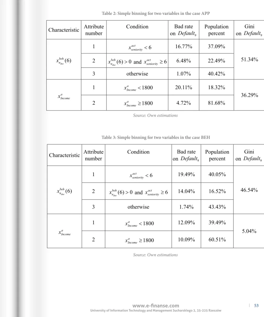
Let us consider the typical scoring models building process, for example on the behavioral sub-portfolio. Because both cases are based on two variables: one application and one behavioral, let only the set of these two variables be considered. To indicate the extreme instability of the models they are being analyzed with the target variable

Default

₉.

Every variable is segmented or binned for the attributes described in tables 2 and 3.

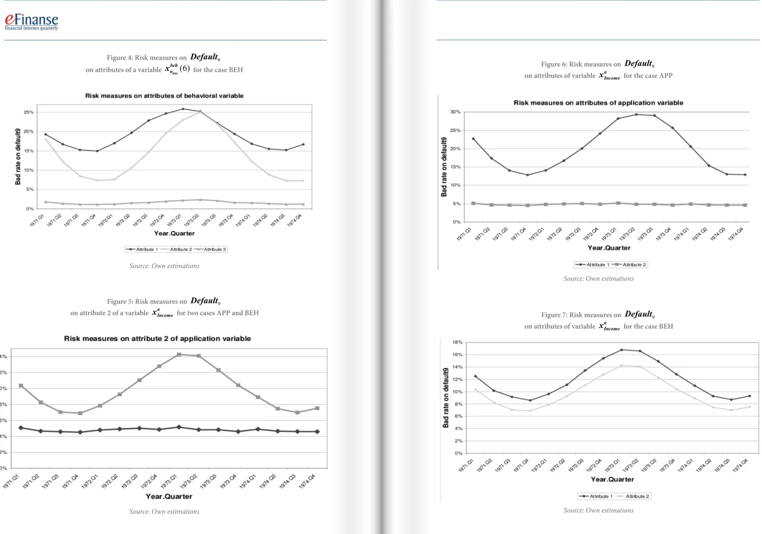
In the case of an unstable application variable (APP) studying igure 6 conirms, what may be expected, that attribute 2 is very stable during this time and accounts from that group are not oversensitive to crisis changes, contrary to attribute 1, which is extremely unstable. he same groups, in the case of unstable behavioral variable (BEH), are both unstable, see igure 7. he same group accounts from attribute 2, which are presented in igure 5, allow both cases to indicate in a better way that the APP case can consistently choose accounts that are insensitive to a crisis. Even a data generator is a simpliication of the real data, a conclusion that is extremely useful. Some application data can be proitable in risk management to indicate sub-segments with a stable risk over time.

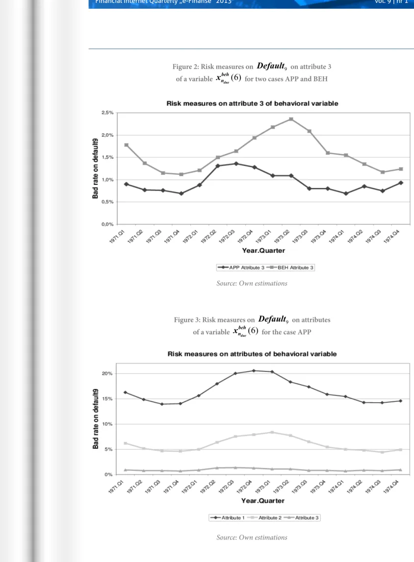
Quite diferent conclusions can be formulated for the behavioral variable

x

n

beh

due

( )

6

_{. In igure 3 risk} evolutions for three attributes of that variable are presented. All of them are unstable. he most stable attribute is number 3. In the case of BEH, that attribute is also unstable, see igure 4. In an attempt to prove this only attributes 3 for both cases are also presented in igure 2. he reader may say that both cases have unstable risk. Even in the case of BEH attribute 3 is expected to have a stable risk, however, due to the rule of migration matrix adjustment, our expectations have not been met. he reason can be found in the correct understanding of the process. A typical scoring approach is based on the principal idea that information available up to the observation point is able to predict the behavior during the outcome period. Up to the observation point if an account has not had any delinquency, the variable

x

_nbeh

due

( )

6 =

0

_{. Ater this point the account may have}

due installments in the next months. It may be adjusted by the macro-economic variable with the result that the group can become unstable.

his idea is very important for further research of the crisis. It should be emphasized that typical scoring methods used on three types of sub-portfolios: APP, BEH and COL cannot reveal in the correct way the rule of crisis adjustment and cannot indicate some sub-segments that are stable over time. Of course, scoring can also be used just as in this paper for the prediction of migration states; namely to be precise, not for default statuses prediction but for transition prediction. he best method is probably the survival analysis (Bellotti and Crook, 2009) or (Crook, 2008) with time covariates (time dependent variables), where in a natural way the factor of being a better or a worse payer is indicated in a set period of time, namely, in the typical scoring model, where the factor is considered only up to the observation point. In the survival model, however it can also be taken into account ater this observation point, so in what may in other words be considered a more realistic way. Many other cases of data generators with more complex rules for

Score

Cycle are made. If both types of variables: application and behavioral are taken together then the case becomes too complicated and there is a widespread unstable property. In that case it is not possible to ind a stable factor. hat conclusion is also very important for crisis analysis, because it describes the nature of a crisis: if it is a major event

and it has an impact on both types of characteristics: behavioral and application, then the risk management can only try to ind some sub-segments more stable

than others or with a maximum risk not exceeding the expected boundary.

Table 2: Simple binning for two variables in the case APP

Table 3: Simple binning for two variables in the case BEH

Source: Own estimations

Characteristic

Attribute

number

Condition

Bad rate

on

Default

₉

Population

percent

Gini

on

Default

₉

x

_nbeh

due

( )

6

1 _x

seniority

act

<

6 16.77%

37.09%

51.34%

2 _x

n

beh

due

( )

6 >

0 _and

_x

seniority

act

≥

6 6.48%

22.49%

3 otherwise

1.07%

40.42%

x

_Incomea

1 x

_Incomea

<

1800

_20.11%

_18.32%

36.29%

2 x

_Incomea

≥

1800

_4.72%

_81.68%

Characteristic

Attribute

number

Condition

Bad rate

on

Default

₉

Population

percent

Gini

on

Default

₉

x

_nbeh

due

( )

6

1 _x

seniority

act

<

6 19.49%

40.05%

46.54%

2 _x

n

beh

due

( )

6 >

0 _and

_x

seniority

act

≥

6 14.04%

16.52%

3 otherwise

1.74%

43.43%

x

_Incomea

1 _x

Income

a

_<

₁₈₀₀

_12.09%

_39.49%

5.04%

2 _x

Income

(6)

Various types of risk measures

Let us deine crisis as a time where risk is the highest. he most popular reporting for risk management is based on bad rates, vintage and low rates. Figure 1 presents bad rates for three diferent sub-portfolios application, behavioral and collection. One low rate is also presented. here is a simple conclusion to be drawn, that crisis does not occur at the same time. Some curves indicate local maximum risk earlier

than others. he diference in time is signiicant and can be as much as 6 months, so it is crucial to remember the nature of reports that can indicate a crisis as quickly as possible. It should be emphasized that bad rates reports present, in a standard way, the evaluation of risk by observation points and a crisis time can occur between the observation point and the end of the outcome period. It appears that low rates reports indicate the crisis time in better way.

Figure 1: Risk measures on

Default

₉ comparison on sub-portfolios: APP, BEH and COL and also with one flow rate

M

23

Default

₉ on attribute 3

of a variable

x

n beh

due

( )

6

_{for two cases APP and BEH}

Default

₉ on attributes

of a variable

x

n beh

due

( )

6

_{for the case APP}

(7)

Default

₉

on attributes of a variable

x

n beh

due

( )

6

_{for the case BEH}

Default

₉

on attribute 2 of a variable

x

_Incomea _{for two cases APP and BEH}

Default

₉

on attributes of variable

x

_Incomea _{for the case APP}

Default

₉

on attributes of variable

x

Income a

for the case BEH

(8)

Implementation

All data were prepared by the SAS System by manual codes written in SAS 4GL used units: Base SAS and SAS/STAT. For the case of unstable behavioral variable - BEH: the Production dataset has 779 993 rows (about 90MB) and the Transaction dataset - 8 969 413 rows (about 400MB). Total time of calculation per case takes about 4 hours.

Conclusions

Even if data are generated by a random-simulated process, which is not realistic, the conclusions give the possibility to better understand the nature of the crisis.

To establish a proitable business it is very important to have a stable process with which to operate. In a Consumer Finance portfolio the main success factor is a correct estimation of credit risk and bad debts. If risk is not stable, a forecast cannot be estimated in the correct way and the business can get into trouble. he last crisis demonstrated that credit risk management was not a straightforward process. he two cases of simulated crisis by random data generators that are presented help explain the complexity of the notion of what makes a crisis and also suggest that only the particular conditions of a crisis can guarantee stable proits for inancial companies. hat is to say, only when the main factors of a crisis are linked with the application characteristics of a customer such as: income, marital status etc. can a stable portfolio that remains proitable in a time of crisis be found. More complex factors will always generate unstable segments and, in these cases, a bank can do little other than accept the fact that it must limit credit production and focus on only the very small and most stable segments, even though this will generate less revenue.

In the irst case, of an unstable application variable like income it is possible to split a portfolio into two parts over a period of time: stable and unstable. In the second case, an unstable behavioral characteristic, the task is more complicated and it is not possible to split it in the same way. Some sub-segments may have better stability but they always luctuate. Moreover, if a crisis is impacted by many factors, both from an application from customer characteristics and from a customer behavioral perspective, it is very diicult to indicate these factors and the crisis is widespread in all reports.

he banking data generator is a new hope in researches aimed at inding the method of comparisons of various credit scoring techniques. It is probable that in the future many randomly generated data will become the new repository for testing and comparisons. he generated data are very useful for various analyses and researches. here are many rows and many bad default statuses, so an analyst can make many good exercises to improve their experience.

References

Bellotti, T., Crook, J. (2009). Credit Scoring with Macroeconomic Variables Using Survival Analysis. Journal of the Operational Research Society, 1699–1707.

BIS-BASEL (2005). International Convergence of Capital Measurement and Capital Standards. Technical Report, Basel Committee on Banking Supervision, Bank For International Settlements. Retrieved from

http://www.bis.org.

BIS-WP14 (2005). Studies on Validation of Internal Rating Systems, Working Paper No. 14, Technical Report, Basel Committee on Banking Supervision, Bank For International Settlements. Retrieved from

http://www.bis.org.

Crook, J. (2008). Dynamic Consumer Risk Models: an Overview. Paper presented at Credit Scoring Conference CRC, Edinburgh. Retrieved from

http://www.business-school.ed.ac.uk/crc/conferences/ conference-archive?a=45349.

Huang, E., Scott, C. (2007). Credit Risk Scorecard Design, Validation and User Acceptance: A Lesson for Modellers and Risk Managers. Paper presented at Credit Scoring Conference CRC, Edinburgh. Retrieved from http://www. business-school.ed.ac.uk/crc/conferences/conference-archive?a=45569.

Huang, E. (2007). Scorecard Speciication, Validation and User Acceptance: A Lesson for Modellers and Risk Managers. Paper presented at Credit Scoring Conference CRC, Edinburgh. Retrieved from

Majer, I. (2010). Application Scoring: Logit Model Approach and the Divergence Method Compared. Warsaw School of Economics - SGH, Working Paper No. 10-06.

Malik, M., homas, L. C. (2009). Modelling Credit Risk in Portfolios of Consumer Loans: Transition Matrix Model for Consumer Credit Ratings. Paper presented at Credit Scoring Conference CRC, Edinburgh. Retrieved from

Mays, E. (2009). Systematic Risk Efects on Consumer Lending Products. Paper presented at Credit Scoring Conference CRC, Edinburgh. Retrieved from

Siddiqi, N. (2005). Credit Risk Scorecards: Developing and Implementing Intelligent Credit Scoring. Wiley and SAS Business Series.

Supramaniam, M., Shanmugam, B. (2009). Simulating Retail Banking for Banking Students. Reports –

Evaluative, Practitioners and Researchers ERIC Identiier: ED503907. Retrieved from

http://www.eric.ed.gov/ERICWebPortal/contentdelivery/ servlet/ERICServlet?accno=ED503907