Annales Geophysicae (2004) 22: 789–806 SRef-ID: 1432-0576/ag/2004-22-789 © European Geosciences Union 2004
Annales
Geophysicae
Quasi-stationary waves in the Southern Hemisphere during El Ni ˜
no
and La Ni ˜
na events
V. Brahmananda Rao, J. P. R. Fernandez, and S. H. Franchito
Centro de Previs˜ao de Tempo e Estudos Clim´aticos, CPTEC. Instituto Nacional de Pesquisas Espaciais, INPE. CP 515, 12201–970, S˜ao Jos´e dos Campos, SP, Brazil.
Received: 26 February 2003 – Revised: 31 July 2003 – Accepted: 4 September 2003 – Published: 19 March 2004
Abstract. Characteristics of quasi-stationary (QS) waves in the Southern Hemisphere are discussed using 49 years (1950–1998) of NCEP/NCAR reanalysis data. A compari-son between the stationary wave amplitudes and phases be-tween the recent data (1979–1998) and the entire 49 years data showed that the differences are not large and the 49 years data can be used for the study. Using the 49 years of data it is found that the amplitude of QS wave 1 has two maxima in the upper atmosphere, one at 30◦S and the other at 55◦S. QS waves 2 and 3 have much less amplitude. Monthly variation of the amplitude of QS wave 1 shows that it is highest in Oc-tober, particularly in the upper troposphere and stratosphere. To examine the QS wave propagation Plumb’s methodol-ogy is used. A comparison of Eliassen-Palm fluxes for El Ni˜no and La Ni˜na events showed that during El Ni˜no events there is a stronger upward and equatorward propagation of QS waves, particularly in the austral spring. Higher upward propagation indicates higher energy transport. A clear wave train can be identified at 300 hPa in all the seasons except in summer. The horizontal component of wave activity flux in the El Ni˜no composite seems to be a Rossby wave prop-agating along a Rossby wave guide, at first poleward until it reaches its turning latitude in the Southern Hemisphere mid-latitudes, then equatorward in the vicinity of South America. The position of the center of positive anomalies in the aus-tral spring in the El Ni˜no years over the southeast Pacific, near South America, favors the occurrence of blocking highs in this region. This agrees with a recent numerical study by Renwick and Revell (1999).
Key words. Meteorology and atmospheric dynamics (cli-matology; general circulation; ocean-atmosphere interac-tions)
Correspondence to:V. Brahmananda Rao (vbrao@cptec.inpe.br)
1 Introduction
Any meteorological variable, φ (for example, geopotential height) can be divided into a time mean and a time deviation:
φ (λ, ϕ, z, t )=φ0(λ, ϕ, z)+φ′(λ, ϕ, z, t ), whereλ,ϕ,zandt are, respectively, longitude, latitude, height and time. φ′is termed as the transient circulation (eddies) and is responsible for weather.φ0can be divided further into a zonal mean and a zonal deviation: φ0(λ, ϕ, z)=φ00(ϕ, z)+φ∗(λ, ϕ, z). φ00 represents the stationary symmetric circulation and is popu-larly known as the Hadley type circulation. φ00 also repre-sents a zonal flow. φ∗is the asymmetric stationary circula-tion and is popularly known as stacircula-tionary waves. Since the stationary waves can change a little (in time) in position and intensity, these are called quasi-stationary (QS) waves. This is the subject of the present paper.
790 V. Brahmananda Rao et al.: Quasi-stationary waves during El Ni˜no and La Ni˜na events
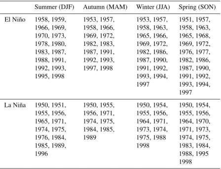
Table 1.El Ni˜no and La Ni˜na years.
Summer (DJF) Autumn (MAM) Winter (JJA) Spring (SON)
El Ni˜no 1958, 1959, 1953, 1957, 1953, 1957, 1951, 1957, 1966, 1969, 1958, 1966, 1958, 1963, 1958, 1963, 1970, 1973, 1969, 1972, 1965, 1966, 1965, 1968, 1978, 1980, 1982, 1983, 1969, 1972, 1969, 1972, 1983, 1987, 1987, 1991, 1982, 1986, 1976, 1977, 1988, 1991, 1992, 1993, 1987, 1990, 1982, 1986, 1992, 1993, 1997, 1998 1991, 1992, 1987, 1990, 1995, 1998 1993, 1994, 1991, 1992, 1997 1993, 1994,
1997
La Ni˜na 1950, 1951, 1950, 1955, 1950, 1954, 1950, 1954, 1955, 1956, 1956, 1971, 1955, 1956, 1955, 1956, 1965, 1971, 1974, 1975, 1964, 1971, 1964, 1970, 1974, 1975, 1984, 1985, 1973, 1974, 1971, 1973, 1976, 1984, 1989 1975, 1988 1974, 1975, 1985, 1989, 1998 1983, 1984,
1996 1988, 1995
1998
More recently, Hurrell et al. (1998) discussed the charac-teristics of stationary waves in the SH, and Kiladis and Mo (1998) discussed their interannual variability. As in Randel (1988), Hurrell et al. (1998) found that at 500 hPa wave 1 reaches its peak between 50◦S and 60◦S in both winter and summer. They noted that wave 1 over the southern oceans closely follows the pattern of the latitude anomalies of tem-perature, suggesting the importance of surface thermal forc-ing. Hurrell et al. (1998) also found that the interannual vari-ability is largest in the Pacific, where the influence of the southern oscillation is highest.
Kiladis and Mo (1998) studied the interannual variability of QS waves in the SH using empirical orthogonal function (EOF) analysis. The wave train-like nature of these EOF modes (see Fig. 8.3c of Kiladis and Mo, 1998) suggests the propagation of Rossby wave energy with a source region in the subtropics. Seasonal composite of 500 hPa height anoma-lies for warm (El Ni˜no) events (see Fig. 8.4 of Kiladis and Mo, 1998) also strongly suggests the Rossby wave propa-gation. A ridge in the southeast Pacific associated with the wave train during the warm events is favorable for blocking in this region and the reverse happens during cold events. Rutllant and Fuenzalida (1991) and Marques and Rao (2000) showed the connection between blocking over the southeast Pacific and ENSO (El Ni˜no-Southern Oscillation). Using a barotropic numerical model, Renwick and Revell (1999) showed that the tropical convective heating associated with the OLR (outgoing longwave radiation) anomaly, presum-ably generated during ENSO events, forces a Rossby wave train which is responsible for higher blocking over the south-east Pacific during El Ni˜no events. In the present study we propose to test the hypothesis of Renwick and Revell (1999)
observationally. We use Plumb’s (1985) approach to exam-ine the three-dimensional propagation of QS waves in the SH, giving emphasis for the El Ni˜no and La Ni˜na events.
2 Data source and methodology
In the present study we use monthly mean values of the geopotential height φ for the period 1950–1998. These data were obtained from NCEP (National Centers for En-vironmental Predictions)/NCAR (National Center for Atmo-spheric Research) reanalysis and are available at 1000, 925, 850, 700, 600, 500, 400, 300, 250, 200, 150, 100, 70, 50, 30, 20 and 10 hPa levels, at 2.5◦×2.5◦(latitude×longitude) in-tervals. For a detailed description of the NCEP/NCAR data assimilation method, see Kalnay et al. (1996).
In our case time mean is taken over a period of three months. We can write the zonal wave components forφ∗
as:
φ∗k(λ, ϕ, p)=Ak(ϕ, p)cos[(kλ+αk(ϕ,p))], (1)
where k is the wave number,Ak, the amplitude andαkis the
phase. In our case,k=1, 20.
The values of temperature T, zonal (u) and meridional
V. Brahmananda Rao et al.: Quasi-stationary waves during El Ni˜no and La Ni˜na events 791
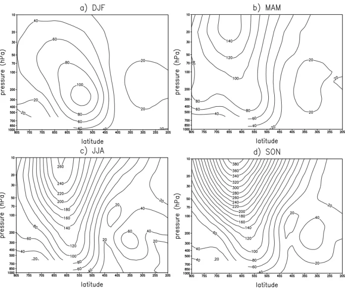
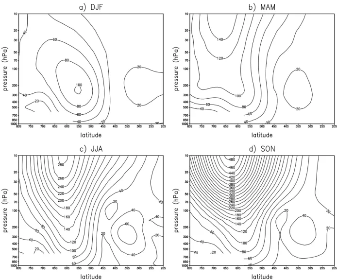
Fig. 1.Amplitudes of QS wave 1 (m) in the data set for the period 1950–1998 for:(a)DJF,(b)MAM,(c)JJA and(c)SON. Contour interval is 20 m.
density, in order to make them visible throughout the strato-sphere. The differences are small if the wind and temperature from NCEP/NCAR reanalysis data are directly used.
The list of El Ni˜no and La Ni˜na episodes was obtained from NCEP (http://www.cpc.noaa.gov/products/ analysis monitoring/ensostuff/). For compiling this list it was attempted to classify the intensity of each event by fo-cusing on a key region of the tropical Pacific (along the equa-tor from 150◦W to the date line). The process of classifica-tion was primarily subjective using reanalyzed sea surface temperature (SST) analyses produced at the NCEP/Climate Prediction Center (CPC) and at the United Kingdom Meteo-rological Office. In the period considered (1950–1998) there are 16 El Ni˜no summers (December, January and February) and 13 La Ni˜na summers. There are 14 El Ni˜no autumns (March, April and May) and 9 La Ni˜na autumns. There are 17 El Ni˜no winters (June, July and August) and 11 La Ni˜na winters. Finally, there are 19 El Ni˜no springs (September, October and November) and 15 La Ni˜na springs. The list of these years is given in Table 1.
3 Characteristics of QS waves
In the present study we used data from 1950 through 1998. Before the advent of meteorological satellites the data were sparse in the SH. Thus, it would be necessary to verify the differences in characteristics of QS waves in the data for 1950–1998 and in recent data. Figure 1 shows the am-plitude of QS wave 1 for different seasons for the periods 1950 through 1998. The corresponding amplitude values for the period 1979 through 1998 are shown in the Appendix (Fig. A1). The magnitude and distribution of the amplitudes of wave 1 in DJF and MAM are very similar in both data sets. Although the distribution in JJA and SON is very similar, the magnitude is slightly higher in spring in the recent data. The differences in amplitudes of wave 1 between the two periods are not entirely due to the improvement of data coverage in recent years. Part of the differences could be due to natural interannual variability.
792 V. Brahmananda Rao et al.: Quasi-stationary waves during El Ni˜no and La Ni˜na events
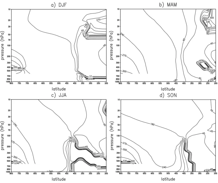
Fig. 2.Same as Fig 1, but for the phase (degrees).
is shown in the Appendix (Fig. A2). The phase distribution is also very similar, except for a small difference in sum-mer, when the amplitude of wave 1 is weakest. Amplitudes of waves 2 and 3 (figures not shown) are also very similar in magnitude and distribution. The amplitude of wave 2 is slightly less and that of wave 3 is slightly more in the re-cent data set. The distribution and magnitude of wave 3 is very similar in both data sets. The phases of waves 2 and 3 are similar in winter in both data sets and slightly differ-ent in other seasons. Wave 1 explains about 90% of the total variance in the geopotential field and all other waves (mostly waves 2 and 3) together explain the remaining 10%. Since the most dominant characteristics of amplitude and phase, particularly of wave 1, are similar in the data set for 1950– 1998 and in the recent data set for 1979–1998, we propose to use the total period of 49 years to study the characteristics of stationary waves in the SH.
Figure 1 shows several interesting characteristics. In sum-mer in the upper troposphere there are two maxima, one at
30◦S and another at 55◦S. The value in the higher latitudes is much larger than that in the subtropics. A comparison with the values in other seasons shows that the QS wave 1 is trapped in the lower atmosphere in summer, while in other seasons it propagates into the stratosphere. In spring the am-plitude values in the lower stratosphere are highest.
V. Brahmananda Rao et al.: Quasi-stationary waves during El Ni˜no and La Ni˜na events 793
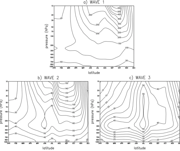
Fig. 3.Monthly variation of the amplitudes (m) of QS waves 1(a), 2(b)and 3(c)at 60◦S. Contour interval is : (a) 50 m, (b) 10 m, and (c) 5 m.
presence of easterlies in the stratosphere in DJF (figure not shown) does not permit the vertical propagation of QS waves, (Charney and Drazin, 1961). Again, in JJA the strong west-erlies are not favorable for vertical propagation. The decreas-ing of westerlies in sprdecreas-ing is favorable for the vertical propa-gation of QS waves and this propapropa-gation is connected to the final warming in the SH stratosphere. From Fig. 2 it can be seen that the phase angle of wave 1 does not change much in the lower troposphere, while in the upper troposphere and stratosphere it decreases with height, indicating a westward inclination. Westward inclination is better defined in win-ter and spring. This westward inclination is associated with poleward heat transport and vertical propagation.
Figure 3 shows the monthly variation of amplitude of QS waves 1, 2 and 3 at 60◦S. At this latitude, the maximum amplitude (100 m) of QS wave 1, in the troposphere is in August, and the maximum amplitude in the stratosphere is in October (550 m). In the stratosphere there is a secondary maximum in July (300 m). The lowest value of amplitudes of
QS wave 1 is found in summer (50 m). The monthly variation of the amplitude of QS wave 2 is similar to that of QS wave 1 except that the amplitudes are less and in the stratosphere in October they are about the same as those of QS wave 1.
The monthly variation of QS wave 3 is very different. A clear winter (July) maximum is found both in troposphere and stratosphere. Compared to QS waves 1 and 2 the ampli-tudes of QS wave 3 are much less. As we have seen earlier (Fig. 3), QS wave 3 is essentially trapped in the troposphere and lower stratosphere. Thus, from the above discussion we can infer the contribution of QS wave 1 for the zonal variance ofφ∗is by far the most dominant.
794 V. Brahmananda Rao et al.: Quasi-stationary waves during El Ni˜no and La Ni˜na events
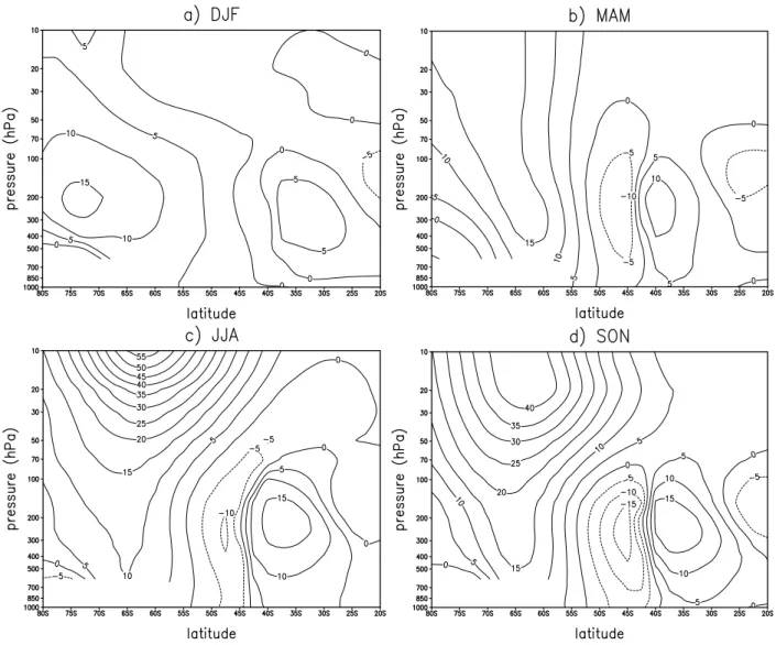
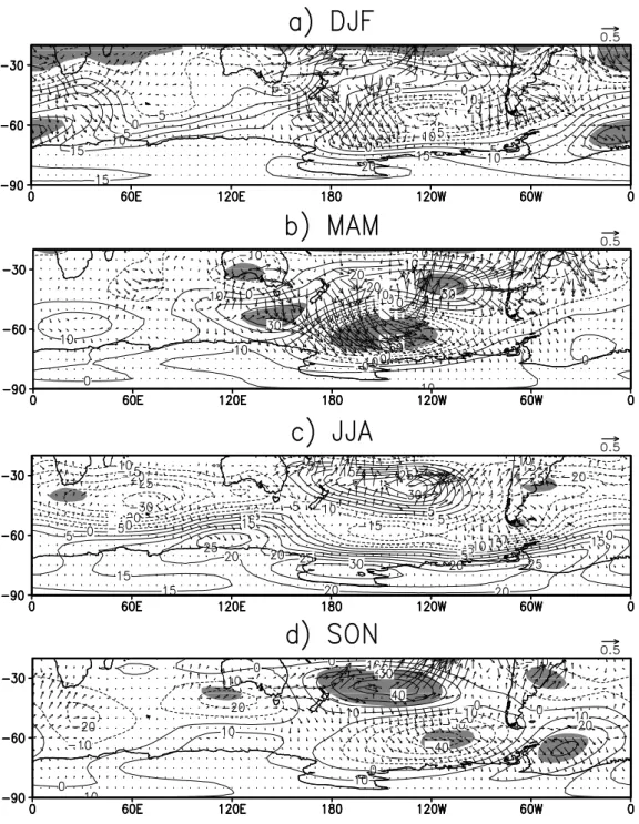
Fig. 4.Difference of amplitude of QS wave 1 (m) between El Ni˜no composite and the mean for:(a)DJF,(b)MAM,(c)JJA, and(d)SON. Contour interval is 5 m.
Figure 4 shows the difference in amplitude of QS wave 1 between El Ni˜no composite and the mean for the four sea-sons. The differences are small in DJF and MAM. In JJA and SON there is an increase in the higher latitudes, particularly in the stratosphere. In the mid-latitudes in the troposphere there is a slight decrease and in the subtropics there is an in-crease. The differences in the La Ni˜na composite (figure not shown) are in general opposite to those of El Ni˜no.
In the EP fluxes for El Ni˜no and La Ni˜na periods (fig-ures not shown) large changes are found mostly in the high-latitude spring stratosphere. The general characteristics of the EP fluxes are similar to the known features (e.g. Ed-mon et al., 1980). There is mostly upward propagation of QS waves in the lower levels in mid and high latitudes and then upward and equatorward propagation in the lower stratosphere. As is well known, the upward propagation of QS waves is associated with poleward sensible heat trans-port and the equatorward propagation is associated with
V. Brahmananda Rao et al.: Quasi-stationary waves during El Ni˜no and La Ni˜na events 795
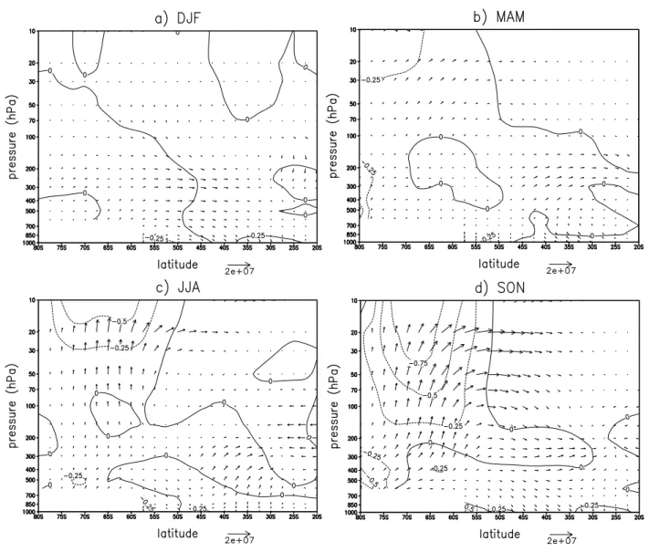
Fig. 5.Zonally-averaged EP flux cross sections for El Ni˜no composite minus the mean for:(a)DJF,(b)MAM,(c)JJA, and(d)SON. Lines indicate divergence of EP flux. The horizontal arrow scale for EP flux is in units of m3s−2and indicated at the bottom of the figures. The EP divergence contour interval is 0.25 m s−1day−1.
about about 35◦S , there is a larger poleward propagation of QS waves in the upper troposphere during El Ni˜no periods in all seasons. Another interesting feature is a larger upward focussing of QS waves in the upper troposphere in the lati-tudes 50◦–65◦S and larger equatorward focussing in spring in the stratosphere.
4 Propagation of QS waves in the SH during El Ni ˜no and La Ni ˜na events
We will use the approach introduced by Plumb (1985) to study the QS wave propagation. This approach has been extensively used in both model and observational studies (Karoly et al., 1989; Lau and Peng, 1992; Schubert et al., 1993; Quintanar and Mechoso, 1995). For small-amplitude
waves on a zonal mean flow, the conservation relationship for stationary wave activity (Plumb, 1985) may be written as
∂As/∂t+ ∇ ·Fs =Cs (2)
whereAs is the stationary wave activity,
As =
1 2p
q∗2 1
asinϕ
∂(Qsinϕ) ∂ϕ
+p E
U. (3)
Fsis the three-dimensional flux of stationary wave activity,
Fs =pcosϕ (
v∗2− 1 2asin 2ϕ
∂(v∗φ∗)
∂λ ,
−u∗v∗− 1 2asin 2ϕ
∂(u∗φ∗)
796 V. Brahmananda Rao et al.: Quasi-stationary waves during El Ni˜no and La Ni˜na events
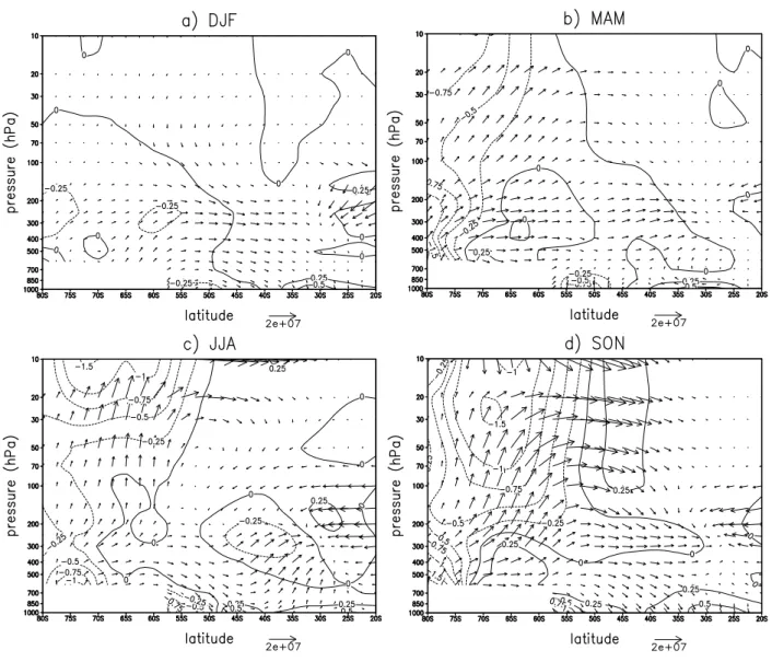
Fig. 6.Same as Fig. 5, but for El Ni˜no minus La Ni˜na.
2sinϕ S
"
v∗T∗− 1 2asin 2ϕ
(T∗φ∗)
∂λ #)
(4)
andCs is a nonconservative source-sink term that includes
diabatic and frictional effects and interactions with transient eddies. The overbar represents a time-average and the quan-tities with asterisks denote departures from the zonal aver-age;pis the pressure,Qandq∗are the zonal mean and per-turbation quasi-geostrophic potential vorticity,Uis the zonal mean flow,E is the wave energy density,u∗ andv∗are the eddy zonal and meridional geostrophic wind components,a
is the Earth’s radius,φis the geopotential,T is the temper-ature,is the angular rotation rate of the Earth andS is a time and area averaged static stability.
Plumb (1985) showed that for steady, conservative waves
Fs is nondivergent and that for slowly varying almost plane
waves, Fs is parallel to the group velocity. In general, the
starred (wave) quantities are evaluated from time averages (over a season) in which case the time-derivative in
expres-sion (2) is relatively small and wave sources (sinks) are asso-ciated with regions whereFsis divergent (convergent). Since Fsis derived under the quasi-geostrophic assumption, its
va-lidity is questionable in low latitudes and also one should be careful in interpreting the short-scale quasi-stationary waves (Quintanar and Mechoso, 1995).
Figures 7 and 8 show the horizontal component of Fs (Hc) and the geopotential height anomalies (El Ni˜no or La
Ni˜na minus the mean) for the El Ni˜no and La Ni˜na compos-ites, respectively. Shaded areas show the significance at the 95% confidence level. In summer (Fig. 7a)Hcis generally
weak compared to the other seasons. The height anomalies show a high (positive center) over southern South America and a weak low to the northwest of this. Hc vectors
indi-cate southeastward wave propagation to the west of southern South America. Divergence of vectors in this region sug-gests a source of QS waves. Over the low to the northwest,
Hcvectors indicate equatorward propagation. As the season
V. Brahmananda Rao et al.: Quasi-stationary waves during El Ni˜no and La Ni˜na events 797
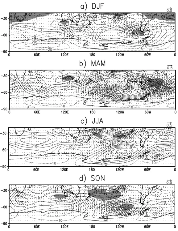
Fig. 7.Horizontal component of QS wave activity (Hc) and geopotential height anomalies (El Ni˜no minus the mean) at 300 hPa for the El Ni˜no composites for:(a)DJF,(b)MAM,(c)JJA, and(d)SON. Contour interval of height anomalies for (a), (b) and (c) is 5 m, and for (d) 10 m. Vectors are in m2s−2.
(highs and lows) in the remaining three seasons is similar. A positive anomaly can be seen over southern Australia, a nega-tive anomaly to the east and again, a posinega-tive anomaly to the southeast over southeastern Pacific. This is similar to what Karoly (1989) and Karoly et al. (1989) noted. TheHc vec-tors in this region show a wave propagation poleward from southern Australia to the southeast and then equatorward in the vicinity of South America. To the west of South America in MAM strong divergence ofHcvectors is seen, suggesting
a stationary wave source. In other seasons the wave activity is weak in this region.
In the La Ni˜na composite (Fig. 8) the height anomalies are in general opposite to those noted in the El Ni˜no composite. Again, the wave activity, as indicated by the magnitude of the
Hc vector, is strong in autumn, particularly in the south
Pa-cific. Hcvectors in autumn indicate wave propagation from
798 V. Brahmananda Rao et al.: Quasi-stationary waves during El Ni˜no and La Ni˜na events
Fig. 8.Same as Fig. 7, but for the La Ni˜na composites.
Pacific American sectors seems to be a preferred route of energy dispersion (Ambrizzi and Hoskins, 1997). The strong divergence ofHcvectors to the southeast of Australia
indi-cate a source of QS waves. In winter the wave activity is not strong. This is somewhat different from what Karoly (1989) noted. He noted the wave pattern in winter. Also Karoly (1989) used only 3 ENSO events and only for the winter and summer seasons. In the present work we use a much larger sample of ENSO events and study the wave propagation in all four seasons. Further Karoly (1989) did not discuss La Ni˜na cases explicitly.
V. Brahmananda Rao et al.: Quasi-stationary waves during El Ni˜no and La Ni˜na events 799 mature phases of El Ni˜no events (such as 1982, 1983, 1997
and 1998) are joined together and so it is more likely that the base state in MAM could be favoring the QS wave propaga-tion during ENSO events. Hoskins and Ambrizzi (1993) and Ambrizzi et al. (1995) have shown the importance of base state on the propagation of QS Rossby waves.
In a recent study, Renwick and Revell (1999) noted a higher incidence of blocking in the southeast Pacific during the El Ni˜no events in the austral spring. Making numeri-cal experiments with a linearized barotropic model they sug-gested that the enhanced blocking over the southeast Pacific is forced by a particular Rossby wave train triggered by an OLR anomaly (diabatic heating or upper level divergence), presumably generated during the El Ni˜no events. Our results seem to corroborate this hypothesis. Also in Fig. 7a the cen-ter of positive anomalies is seen over the southeast Pacific. This positive center is associated with higher frequency of blocking highs in this region. In Fig. 8d a negative anomaly center can be seen. This suggests a decrease in the frequency of blocking highs in this region during the La Ni˜na events in spring. The predisposition towards blocking over this region during the El Ni˜no events and vice versa during the La Ni˜na events was pointed out by Kiladis and Mo (1998) as well. However, in the present study it is shown that the formation of a positive center over southeast Pacific is associated with stationary wave propagation. The vertical component ofFs
for the El Ni˜no and La Ni˜na composites (figures not shown) did not show large differences, except that during the El Ni˜no events there seems to be higher vertical propagation.
To see the vertical variation of the QS wave configuration,
Hc vectors and the height anomalies are computed for 200 and 500 hPa. These are shown in the Appendix (Figs. A3– A6). The characteristics of height anomalies andHcvectors
are very similar to what was seen earlier in Figs. 7 and 8. This shows that the configuration of QS waves are essentially barotropic in nature, and a barotropic model will be able to simulate well the propagation of QS waves. Indeed, Renwick and Revell (1999) were successful in simulating QS Rossby wave propagation using a barotropic model.
5 Summary and conclusions
In this paper we studied the characteristics of QS waves in the SH using 49 years (1950–1998) of NCEP/NCAR reanal-ysis data. Earlier studies (e.g. Quintanar and Mechoso, 1995) used much less data. A comparison between the characteris-tics of QS waves in the 49 years data and recent data (1979– 1998), which included satellite soundings, showed that the differences are not large and the entire 49 years of data can be used with confidence. The amplitude of QS wave 1 has two maxima, one at 30◦S and the other at 55◦S. The maxi-mum at 55◦S is noted in all four seasons and this maximum is more than double that in the subtropics. The maximum in the subtropics is strongest in the austral winter, while the maximum at 55◦S is strongest in spring. Except in summer, the QS wave 1 amplitude increases from the troposphere into
the stratosphere, indicating a vertical propagation. QS waves 2 and 3 have much less amplitudes. Monthly variation of the amplitude of QS wave 1 clearly shows that it is highest in October, particularly in the upper troposphere and the lower stratosphere.
The difference between the El Ni˜no and La Ni˜na years and the mean showed that during the El Ni˜no years there is an in-crease in the amplitude of QS 1 in winter and spring in the higher latitudes, mainly in the stratosphere. Both in winter and spring there is an increase of the amplitude of QS wave 1 in the troposphere in the subtropics. During the La Ni˜na years there is a decrease in the amplitude of QS wave 1 in the troposphere and stratosphere in winter. A comparison of EP fluxes for El Ni˜no and La Ni˜na periods showed that dur-ing the El Ni˜no period there is a stronger upward and equa-torward focussing of QS waves, particularly in spring. Since the EP vectors are parallel to the direction of energy prop-agation, the differences between the El Ni˜no and La Ni˜na periods give the direction of differences in energy transport.
To examine the QS wave propagation for El Ni˜no and La Ni˜na periods Plumb’s (1985) methodology is used. A clear wave train can be identified at 300 hPa throughout the year, except in summer. The horizontal component of wave activity in the El Ni˜no composite showed a Rossby wave propagation along a Rossby wave guide, at first pole-ward until it reaches its turning latitude in the SH mid-latitudes, then equatorward in the vicinity of the South Amer-ica (Hoskins and Ambrizzi, 1993). This path over the Pacific-American sectors seems to be a prefered route of energy dispersion (Ambrizzi and Hoskins, 1997). Ambrizzi and Hoskins (1997) noted the existence of a wave guide along the South Pacific jet and into the subtropics of the South At-lantic during the austral summer. But our results show that the wave train is not clearly defined in summer.
800 V. Brahmananda Rao et al.: Quasi-stationary waves during El Ni˜no and La Ni˜na events
Appendix
V. Brahmananda Rao et al.: Quasi-stationary waves during El Ni˜no and La Ni˜na events 801
802 V. Brahmananda Rao et al.: Quasi-stationary waves during El Ni˜no and La Ni˜na events
V. Brahmananda Rao et al.: Quasi-stationary waves during El Ni˜no and La Ni˜na events 803
804 V. Brahmananda Rao et al.: Quasi-stationary waves during El Ni˜no and La Ni˜na events
V. Brahmananda Rao et al.: Quasi-stationary waves during El Ni˜no and La Ni˜na events 805
806 V. Brahmananda Rao et al.: Quasi-stationary waves during El Ni˜no and La Ni˜na events
Acknowledgements. One of the authors (J. P. R. Fernandez) was supported by Fundac¸˜ao de Amparo `a Pesquisa do Estado de S˜ao Paulo (FAPESP/Processo 98/16035-6). Thanks are due to the two referees for their useful suggestions.
Topical Editor U.-P. Hoppe thanks two referees for their help in evaluating this paper.
References
Ambrizzi, T. and Hoskins, B. J.: Stationary Rossby wave propaga-tion in a baroclinic atmosphere, Quart. J. Roy. Meteor. Soc., 123, 919–928, 1997.
Ambrizzi, T., Hoskins, B. J., and Hsu, H. H.: Rossby wave propaga-tion and teleconnecpropaga-tion patterns in the austral winter, J. Atmos. Sci., 52, 3661–3672, 1995.
Charney, J. G. and Eliassen, A.: A numerical method for predicting the perturbations of the middle-latitude westerlies, Tellus, 1, 38– 54, 1949.
Charney, J. G. and Drazin, P. G.: Propagation of planetary-scale disturbances from the lower into upper atmosphere, J. Geophys. Res., 66, 83–109, 1961.
Edmon, H. J., Hoskins, B. J., and McIntyre, M. E.: Eliassen-Palm cross sections for the troposphere, J. Atmos. Sci., 37, 2600–2616, 1980.
Eliassen, A. and Palm, E.: On the transfer of energy in stationary mountain waves. Geofys. Publ., 22, No. 3, 1–23, 1961.
Hartman, D. L.: Stationary planetary waves in the Southern Hemi-sphere, J. Geophys. Res., 82, 4930–4934, 1977.
Holopainen, E. O.: On the dynamic forcing of the long term flow by large-scale Reynold’s stresses in the atmosphere, J. Atmos. Sci., 35, 1596-1604, 1978.
Holopainen, E. O., Rontu, L., and Lau, N.-C.: The effect of large-scale transient eddies on the mean flow in the atmosphere, J. At-mos. Sci., 39, 1702-1984, 1982.
Hoskins, B, J. and Ambrizzi, T.: Rossby wave propagation on a realistic longitudinally varying flow, J. Atmos. Sci., 50, 1661– 1671, 1993.
Hurrell, J. W., van Loon, H., and Shea, D. J.: The mean state of the troposphere, in: Meteorology of the Southern Hemisphere, editd by Karoly, D. J. and Vincent, D. G., Meteorological Monographs, American Meteorological Society, 1–46, 1998.
Kalnay, E., Kanamitsu, M., and Kistler, R. et al.: The NCEP/NCAR 40-year reanalysis project, Bull. Amer. Meteor. Soc., 77, 437– 471, 1996.
Karoly, D. J.,: Southern Hemisphere circulation features associated with El-Ni˜no-southern oscillation events, J. Climate, 2, 1239– 1252, 1989.
Karoly, D. J., Plumb, R. A., and Ting, M.: Examples of horizontal propagation of quasi-stationary waves, J. Atmos. Sci., 46, 2802– 2811, 1989.
Kiladis. G. N. and Mo, K. G.: Interannual and intraseasonal vari-ability in the Southern Hemisphere, in: Meteorology of the Southern Hemisphere, edited by Karoly, D. J. and Vincent, D. G., Meteorological Monographs, American Meteorological So-ciety, 307–336, 1998.
Lau, K. M. and Peng, L.: Dynamics of atmospheric teleconnections during the northern summer, J. Climate, 5, 140–158, 1992. Marques, R. F. C. and Rao, V. B.: Interannual variations of
block-ings in the Southern Hemisphere and their energetics, J. Geo-phys. Res., 105, D4, 4625–4636, 2000.
Mechoso, C. R. and Hartman, D. L.: An observational study of travelling planetary waves in the Southern Hemisphere, J. Atmos. Sci, 39, 1921–1935, 1982.
Plumb, R. A.: On the three-dimensional propagation of stationary waves, J. Atmos. Sci., 42, 217–229, 1985.
Quintanar, A. I. and Mechoso, C. R.: Quasi-stationary waves in the Southern Hemisphere, Part I: Observational data, J. Climate, 8, 2659–2672, 1995.
Randel, W. J.: A evaluation of winds from geopotential height data in the stratosphere, J. Atmos. Sci., 44, 3097–3120, 1987. Randel, W. J.: The seasonal evolution of planetary waves in the
Southern Hemisphere stratosphere and troposphere, Quart, J. Roy. Meteor. Soc., 114, 1385–1409, 1988.
Renwick, J. A. and Revell, M. J.: Blocking over the South Pacific and Rossby wave propagation, Mon. Wea. Rev., 127, 2233–2247, 1999.
Rutllant, J. and Fuenzalida, H.: Synoptic aspects of the central Chile rainfall variability associated with the southern oscillation, Int. J. Climatol., 11, 63–76, 1991.
Schubert, S. D., Suarez, M., Park, C.-K , and Moorthi, S.: GCM simulations of intraseasonal variability in the Pacific/North American region, J. Atmos. Sci., 50, 1991–2007, 1993. Smagorinsky, J.: The dynamical influences of large scale heat
sources and sinks on the quasi-stationary mean motions of the atmosphere, Quart. J. Roy. Meteor. Soc., 79, 342–366, 1953. Trenberth, K. E.: Planetary waves at 500 hPa in the Southern
Hemi-sphere, Mon. Wea. Rev., 108, 1378–1389, 1980.