© Author(s) 2016. CC Attribution 3.0 License.
Using ground-penetrating radar, topography and
classification of vegetation to model the sediment and
active layer thickness in a periglacial lake catchment,
western Greenland
Johannes Petrone1, Gustav Sohlenius2, Emma Johansson1,5, Tobias Lindborg1,3, Jens-Ove Näslund1,5, Mårten Strömgren4, and Lars Brydsten4
1Swedish Nuclear Fuel and Waste Management Company, Box 250, 101 24, Stockholm, Sweden
2Geological Survey of Sweden, Box 670, 751 28, Uppsala, Sweden
3Department of Forest Ecology and Management, Swedish University of Agricultural Science,
90183 Umeå, Sweden
4Department of Ecology and Environmental Science, Umeå University, 901 87 Umeå, Sweden
5Department of Physical Geography, Stockholm University, 106 91 Stockholm, Sweden
Correspondence to:Johannes Petrone ([email protected])
Received: 16 May 2016 – Published in Earth Syst. Sci. Data Discuss.: 5 July 2016 Revised: 23 September 2016 – Accepted: 30 October 2016 – Published: 23 November 2016
Abstract. The geometries of a catchment constitute the basis for distributed physically based numerical
mod-eling of different geoscientific disciplines. In this paper results from ground-penetrating radar (GPR) measure-ments, in terms of a 3-D model of total sediment thickness and active layer thickness in a periglacial catchment in western Greenland, are presented. Using the topography, the thickness and distribution of sediments are cal-culated. Vegetation classification and GPR measurements are used to scale active layer thickness from local measurements to catchment-scale models. Annual maximum active layer thickness varies from 0.3 m in wet-lands to 2.0 m in barren areas and areas of exposed bedrock. Maximum sediment thickness is estimated to be 12.3 m in the major valleys of the catchment. A method to correlate surface vegetation with active layer thick-ness is also presented. By using relatively simple methods, such as probing and vegetation classification, it is possible to upscale local point measurements to catchment-scale models, in areas where the upper subsurface is relatively homogeneous. The resulting spatial model of active layer thickness can be used in combination with the sediment model as a geometrical input to further studies of subsurface mass transport and hydrological flow paths in the periglacial catchment through numerical modeling. The data set is available for all users via the PANGAEA database, doi:10.1594/PANGAEA.845258.
1 Introduction
Recent climate warming, and its effect on near-surface hy-drothermal regimes, is predicted to have a pronounced effect in northern latitudes (e.g., Maxwell and Barrie, 1989; Roots, 1989; MacCraken et al., 1990; Burrows et al., 2011; Larsen et al., 2014). In permafrost regions, where parts of the subsur-face stay permanently frozen, one noticeable effect of global warming is a thickening of the active layer (Larsen et al.,
car-bon stored in the permafrost may be released, implying a positive feedback to climate warming (Walter et al., 2006; Schuur et al., 2015).
Dramatic changes in the Arctic during the last decades have, among other things, led to an increase in the length of the melting season and changes in precipitation patterns (Macdonald et al., 2005). To understand future local and re-gional effects of a warming climate in permafrost regions, it is first necessary to understand the present-day conditions and processes. Modeling the active layer and its variation, as well as any underlying sediments, is needed to account for different scenarios in which the active layer will vary in depth when surface conditions are changing. In addition, in-formation regarding the properties and spatial distribution of the sediments and the active layer is valuable when studying the hydrology and mass transport in permafrost regions.
Conventional methods to identify permafrost features or bedrock under Quaternary deposits in permafrost regions, e.g., through boreholes or excavations, can be problematic and time-consuming due to the frozen conditions. In addi-tion, such methods provide limited information on the spatial distribution of such features. Methods for investigating the spatial variability of the active layer include airborne elec-tromagnetic measurements (e.g. Pastick et al., 2013), space-borne interferometric synthetic aperture radar (InSAR) (e.g. Liu et al., 2012) and ground-penetrating radar (GPR) (e.g., Wu et al., 2009; Stevens et al., 2009). In this study we use GPR to investigate shallow sub-surface features, such as sed-iment thickness and the depth of the active layer. GPR sur-veying has been commonly used since the mid-1990s in geo-physical studies that require high vertical resolution with lit-tle or no disturbance in the investigated area (Neal, 2004). The method is also very flexible, as real-time acquisition and interpretation of the data immediately give preliminary results. The suitability of the GPR method to map subsur-face features in periglacial environments is due to the sig-nificantly different electrical properties between ice, water, sediment, bedrock and air. Relative dielectric permittivity is commonly used to determine the wave velocity of electro-magnetic waves transmitted and received from the GPR. The dielectric permittivity is highly influenced by water content (Neal, 2004). It is therefore an effective method to map the permafrost boundary during summer as well as the subsur-face bedrock (i.e., sediment thickness) when the sediments are frozen. Many studies using GPR in permafrost environ-ments have been carried out (e.g., Wu et al., 2009; Stevens et al., 2009), as have studies using GPR to investigate the properties of the active layer (e.g., Ermakov and Starovoitov, 2010; Jørgensen and Andreasen, 2007; Doolitle et al., 1990; Gacitúa et al., 2012). Gacitúa et al. (2012) also showed that the difference in vegetation cover is closely tied to varying moisture content of sediments in periglacial environments.
The studies listed above, however, only focus on single and local profile investigations. The purpose of this study is to draw conclusions about subsurface conditions over larger
areas, such as individual lake catchments. Here we use GPR to gather information about the relative dielectric permittivity (i.e., water content) of the sediments above the permafrost. The water content of the soil influences the composition of vegetation and the thickness of the active layer. A correla-tion between active layer thickness (ALT) and vegetacorrela-tion can therefore be expected. This correlation is used to construct a model of the spatial distribution and variation in the active layer and upscale results from concentrated measurements to a catchment-wide model.
In the present study we use GPR during different seasons to measure the depth to bedrock and ALT within a small lake catchment, in this paper referred to as Two Boat Lake (TBL), situated close to the Greenland Ice Sheet (Fig. 1). The sed-iment thickness within the catchment has been correlated to topography – i.e., the thickest sediment layers are found in flat areas of the valley floors (Petrone, 2013). This estab-lished relationship, in combination with field surveys and sampling, forms the basis for the construction of a model of sediment thickness and general stratigraphy. For the ac-tive layer we analyze the results in combination with probe measurements to estimate permittivity of the underlying sed-iments and with remote sensing to classify the vegetation. The relationship between vegetation and permittivity (Gac-itúa et al., 2012) is used to calculate active layer depth for all GPR measurements. The result is a 3-D model of sediment thicknesses, sediment types and maximum thicknesses of the
active layer, at catchment scale (∼1–2 km2). Data on
mete-orological and hydrological conditions and properties of the TBL catchment were published by Johansson et al. (2015), and Lindborg et al. (2016) published data on biogeochem-istry from TBL. These new data on ALT and sediment thick-ness constitute valuable complementary input data when set-ting up distributed physically based hydrological and biogeo-chemical numerical models of the catchment. Since the ac-tive layer model is superimposed on the sediment model, it is also possible to study effects of a changing climate by vary-ing the active layer depth. An increased depth of the active layer activates new hydrological flow paths above the present permafrost. The developed 3-D model presented in this study may constitute a geometrical input to other models studying the effect of those processes. By correlating different types of vegetation classes found in periglacial environments to sub-surface wetness conditions, we construct models extending outside of the initial point measurements.
2 Methods
400 000 440 000 480 000 520 000 560 000 7 340 000
7 370 000
7 400 000
7 430 000
7 460 000
7 490 000
Kangerlussuaq
Itilleq
Arctic Circle
Greenland Ice Sheet
Two Boat Lake
Søndre Strømfjord
Arctic ircle
Coord. System: WGS 1984 UTM Zone 22N
C
Figure 1.Map showing the location of the study site (Two Boat Lake), accessible from the nearby town of Kangerlussuaq (modified from
Johansson et al., 2015).
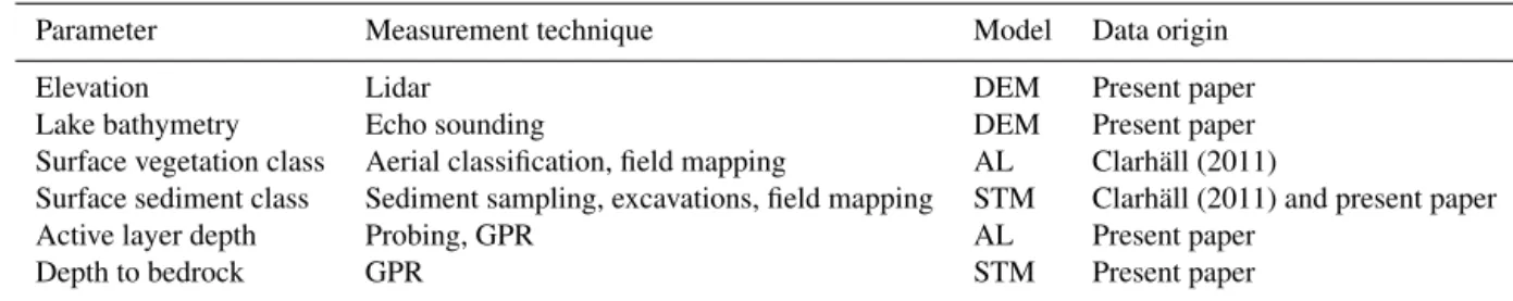
Table 1.List of equipment and in which resulting model the data are used. DEM: digital elevation model; AL: active layer model; STM:
sediment thickness model.
Parameter Measurement technique Model Data origin
Elevation Lidar DEM Present paper
Lake bathymetry Echo sounding DEM Present paper
Surface vegetation class Aerial classification, field mapping AL Clarhäll (2011)
Surface sediment class Sediment sampling, excavations, field mapping STM Clarhäll (2011) and present paper
Active layer depth Probing, GPR AL Present paper
Depth to bedrock GPR STM Present paper
the sediments. All field investigations were carried out in the catchment of TBL; a general site description is provided in Sect. 2.1.1 below, followed by a more detailed description of the Quaternary geology of the catchment in Sect. 2.1.2. The investigation techniques and modeling methodologies for the DEM, the thickness of the active layer and the sed-iment thickness are described in Sect. 2.2–2.4. All data pre-sented in the present paper, as well as information on asso-ciated measurement techniques and the model in which the data are used, are listed in Table 1.
2.1 Site description
2.1.1 General site description
The TBL catchment (described in Johansson et al., 2015), is situated in close proximity to the Greenland Ice Sheet
and approximately 30 km from the settlement of Kangerlus-suaq, western Greenland (Fig. 1). The Kangerlussuaq region, reaching from the coast towards the ice sheet, contains an
ex-tensive (>150 km wide) ice-free area dominated by an
undu-lating periglacial tundra environment with numerous lakes.
The annual corrected precipitation (P) recorded by the local
automatic weather station in the TBL catchment, installed in April 2011, was 365 mm in 2012 and 269 mm in 2013 (Jo-hansson et al., 2015). This is approximately twice as much as the precipitation measured in Kangerlussuaq for the cor-responding periods (Cappelen, 2014). The mean annual air
temperature (MAAT) at TBL is−4.3◦C for the same period
(Johansson et al., 2015) and−4.8◦C in Kangerlussuaq
(Cap-pelen, 2014).
Active layer depth Sediment thickness
GPR results (Petrone, 2013) Data collection
GPR data processing
Supervised classification of vegetation Literature
Vegetation
(Clarhäll, 2011)
Probe results
Velocity analysis
Rule set Sediment coverageDEM
Field survey
Active layer depths
Statistical analysis Interpreted reflection times
Conceptual model
Active layer model Sediment thickness model
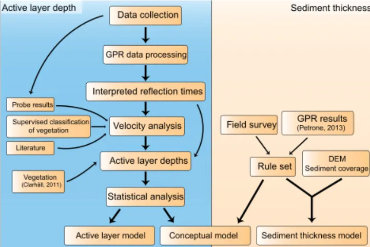
Figure 2.General work flow leading up to the completed models
covering both active layer thickness and regolith thickness.
through taliks, i.e., local areas with no permafrost, often sit-uated below larger lakes (Christiansen and Humlum, 2000). A bedrock borehole below TBL and the results from the in-vestigations made in the instrumented drill hole have shown that the lake is underlain by a through-talik and that the per-mafrost in surrounding land areas reaches a depth of around 300 to 400 m (Harper et al., 2011). The active layer freezes and thaws in cycles directly related to the seasonal variations in air temperature, with a maximum thawed depth at the end of summer.
The area of TBL is 0.37 km2and its catchment covers an
area of 1.56 km2(Johansson et al., 2015). There is a height
difference of around 200 m from the deepest part of the lake
(∼30 m water depth) to the highest point in the southwestern
part of the catchment (Fig. 3).
Most of the catchment has sparse but continuous vege-tation cover, with some exceptions of areas with exposed bedrock or till. Vegetation is in general dominated by dwarf-shrub heath. There are no trees, and the dwarf-shrubs rarely exceed 0.5 m in height. There is a fairly limited number of vascular plant species, but the spatial distribution and density of in-dividual species are highly variable in different parts of the catchment. The vegetation has been classified into several categories (Fig. 3a), based on field surveys and classification in aerial photographs (Clarhäll, 2011). Heath covers a large
portion of the catchment; major plants in this class are
Be-tula nana,Salix glaucaandVaccinium uliginosum. The
veg-etation is classified as eitherBetulaorSalixif any one plant
dominates the coverage. In general, the class heath consists of a mixture of plant species where dwarf shrubs are a signif-icant constituent. Barren surfaces (Fig. 3a), completely lack-ing vegetation, are present in exposed areas where wind has eroded the silt layer and exposed underlying till or bedrock. Grasslands on ridges and exposed dry areas (Fig. 3a) are also scattered around the catchment. The catchment in general constitutes a very dry environment, but a few topographically low areas can be saturated with water during and after events
of high precipitation, as well as when the snowpack melts during springtime. Areas with relatively high soil water con-tent have thus developed and are here termed wetlands.
2.1.2 Quaternary geology of the study area
The geographical distribution of sediment types was deter-mined during field surveys in the summers of 2010 and 2011. Sediment samples were taken from seven locations (Fig. 3b) and analyzed for grain-size distribution. Results from the field observations were used to construct a conceptual model illustrating the stratigraphical distribution of the most com-monly occurring sediment types. The results are partly re-ported by Clarhäll (2011).
The Quaternary geology within the catchment was first described by Clarhäll (2011). An updated sediment map, based on new results from later excavations and field ob-servations, is presented in the present paper (Fig. 3b). The uppermost sediments are dominated by eolian silt, under-lain by till, which is also representative of the regional area (Clarhäll, 2011). Deposition of the eolian silt has occurred since at least ca. 4750 years BP (Willemse et al., 2003), when the ice margin was situated further inland (van Tatenhove et al., 1996). Surficial glacial till and bedrock outcrops can be found in places where erosion has removed the eolian silt. The boundary is often sharp with a scarred surface reveal-ing the underlyreveal-ing till. The till is loosely compacted and is dominated by sand and gravel with a low content of silt and clay, which indicates a marginal deposition in front of the ice sheet (Clarhäll, 2011). Glaciofluvial deposits are also found in several areas, mainly in the northern regions of the catch-ment. Stratigraphical studies have shown that the till contains layers of water laid deposits and the hydrological properties of the till and the glaciofluvial deposits can therefore be re-garded as comparable. In the central and low-lying parts of the major valleys, silt deposition and accumulation of organic material have resulted in areas of peaty silt. The floor of the lake is covered to a large extent by currently accumulating silt. Permafrost-related processes have also led to the devel-opment of ice-wedge polygons in local areas where the sedi-ments are characterized by a relatively high water content.
2.2 Digital elevation model
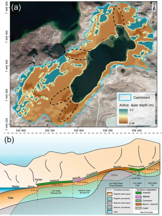
Figure 3. (a)Vegetation map of the catchment outlined in black with defined sub-areas and selected GPR data points.(b) The aerial distribution of sediment classes and bedrock outcrops within the catchment in addition to field measurements. Spatial distributions are from Clarhäll (2011).
The lidar data were collected for a large part of the TBL catchment using a Riegl Z-450 (2000 m range) laser scan-ner. Survey stations and ground control points were surveyed
and georeferenced to geodetic control quality (∼centimeter
precision) using a Leica 1200 GPS receiver processed by
from WGS84 ellipsoid heights to the local elevation datum. The vertical offset between the ellipsoid height and the local
datum is−31.1 m.
Approximately 21 million elevation values were collected during the lidar data measurement. These values were recal-culated to mean values within 1 m cells. In the terrestrial ar-eas not covered by lidar data, elevation data from the previ-ous DEM (Clarhäll, 2011) were used. Lidar data within 2 m from the lake shoreline were removed to obtain a smoother transition between the lake and the terrestrial area in the DEM.
The bathymetric survey of TBL was made with a com-bined echo sounder and GPS (Humminbird 798ci HD SI) at-tached to a boat. Positions, water depth and bottom hardness were stored every second during the measurements. Incor-rect measurements were subsequently removed and in some areas depth data were thinned out to obtain a similar data density over the surveyed area. After these corrections, ap-proximately 18 500 measurements remained. Monitoring of lake level variations was initiated in September 2010 (Jo-hansson et al., 2015). All water depth values from TBL were adjusted to the lake level at the beginning of the monitoring and were converted to the coordinate system used for the li-dar data. Points were added along the lake shoreline every 5 m using the extension of the lake shown in Clarhäll (2011). The lake shoreline was adjusted to the lidar data and a lake level of 336.4 m a.s.l. was determined. The depth data from TBL were recalculated from the lake level, i.e., from depth in meters below 336.4 m a.s.l.
Finally, terrestrial data and depth values were merged to a data set of approximately 1.3 million points. From this data set, a 5 m by 5 m resolution DEM was con-structed. The interpolation of point values was done us-ing the Geostatistical Analysis extension in ArcGIS 10.1. Ordinary Kriging was chosen as the interpolation method (Davis, 1986; Isaaks and Srivastava, 1989). The different data sources and their estimated accuracy are shown in Ap-pendix A. The resulting DEM is available at PANGAEA (doi:10.1594/PANGAEA.845258).
2.3 Thickness surveys of sediments and active layer
The total sediment thickness in the catchment was investi-gated by GPR in April 2011 (Petrone, 2013). A MALÅ X3M shielded antenna GPR system, with a central frequency of 250 MHz, was used. A Trimble R7 GPS was connected to the GPR to log the position of each measurement. Each pro-file was measured by dragging the GPR equipment at con-stant walking speed. The measurements were carried out in straight profiles perpendicular to each other to analyze the spatial variation in sediment thickness. The methodology is thoroughly described in Petrone (2013).
To establish absolute sediment depth values, the start and end points of each transect were situated at or nearby bedrock outcrops. This allowed the bedrock reflector to be
easily identified and continuously traced along the transects. The relationship between sediment thickness and topogra-phy (DEM) constitute the basis for the sediment model. The updated DEM, described in Sect. 2.3, was used to extract the steepness of the topography. The surface sediment map (Fig. 3b) was also used as input to provide the spatial distri-bution of sediment types.
The thickness of the active layer was investigated by prob-ing in 83 points in several transects in August 2011 us-ing a steel rod (Fig. 3b). All points were located in tran-sects at semi-regular intervals covering different soil types, vegetation and topographic properties (such as elevation, slope and aspect). The relevant transects are marked with “1” and “2” in Fig. 3b. An additional GPR survey was car-ried out simultaneously to the probe measurements, using GPR equipment identical to that used during the earlier mea-surements. This survey was concentrated to three sub-areas (Fig. 3a). All GPR profiles related to the active layer sur-veys were processed and analyzed in the same way as in Petrone (2013). Low- and high-frequency noise was reduced by applying dewow and bandpass filters and each profile was geo-referenced. A clear reflector, identified as the reflection of the boundary between thawed and frozen sediments, can be identified in most profiles. In profiles with a less clear and/or discontinuous reflector, or in cases of extremely noisy radargrams, the data were discarded. All remaining selected points, representing the interpreted travel time from the sur-face to the permafrost boundary and back, are seen in Fig. 3a.
2.4 Modeling of active layer depth and sediment thickness
2.4.1 Vegetation class and radar wave velocity correlation
Travel
time
[ns]
0
20
40
60
Distance [m]
Active
layer
depth
[cm] 0
50
100
150
Active layer depth (probe) Active layer depth (modeled)
Wetland
Heath
Shore
Altitude [m a.s.l.]
330 335 340 345 350
(d)
(e)
(f)
0 20 40 60 80 100 120
Distance [m]
0 50 100 150
Altitude [m a.s.l.]
330 335 340
345 Heath
Wetland Betula
Ice-wedge polygon
Active layer depth [cm]
0
25
50
75
Travel time [ns]
0
20
40
0.06 0.057 0.031
0.048
0.031
0.045 0.043 0.055 0.039
0.057 0.058
0.058
Smoothed interpretation from GPR Raw interpretation from GPR
Active layer depth with wave velocity (m ns ) 0.045
Travel time [ns]
20
40
(a)
(b)
(c)
–1
Figure 4.Profile 1 (Fig. 3b) with(a)the raw data from the GPR,(b)probe depths to permafrost and selected permafrost reflectors from
the raw data. Values below probe bars represent the calculated electromagnetic wave velocity at the probe locations and surface vegetation classes as background.(c)Elevation, permafrost features and vegetation. Profile 2 (Fig. 3b) with (d)raw data from the GPR,(e)probe depth to permafrost with modeled depth from raw data and Table 2 as well as vegetation classes in the background.(f)Surface altitude and vegetation along profile.
locations. The corresponding surface altitude and vegetation class variation is shown in Fig. 4c, along with any permafrost features. For clarity, the vegetation classes along the transect shown in Fig. 4c are also included in panel b. Mean values of radar wave velocity were assigned to corresponding
vege-tation classes (heath: 0.059 m ns−1; wetland: 0.045 m ns−1;
Betula: 0.058 m ns−1). Grassland, absent along transect 1,
was assigned a velocity value based on heath and Betula
(0.0585 m ns−1), assumed to be similar in soil water content.
The wave velocity near the shore line (water class) was
as-signed a velocity of 0.05 m ns−1based on saturated silt (Neal,
2004). Assigned velocities and the source for the estimation are presented in Table 2.
2.4.2 Upscaling of active layer depth to catchment scale based on vegetation classes
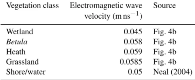
veg-Table 2.Summary of the results from the velocity analysis in Fig. 4.
Vegetation class Electromagnetic wave Source velocity (m ns−1)
Wetland 0.045 Fig. 4b
Betula 0.058 Fig. 4b
Heath 0.059 Fig. 4b
Grassland 0.0585 Fig. 4b
Shore/water 0.05 Neal (2004)
etation maps. The resulting maps provided high-resolution information on vegetation cover over the areas investigated by the GPR and probe measurements.
All reflectors (Fig. 3a), i.e., points within the area with a known travel time for the electromagnetic wave to the permafrost table, were assigned a wave velocity based on Table 2 and the vegetation in that point. The velocity es-timations for each vegetation group, presented in Table 2, were controlled by applying the velocities for each vege-tation group to another transect, transect 2 in Fig. 3b. The processed GPR data, plotted topography and vegetation, as well as the permafrost boundary and probe measurements of transect 2, are shown in Fig. 4d–f. The comparison between measured and modeled values of the active layer thickness
(Fig. 4e) shows good accuracy (R2=0.84) when using the
estimated velocities in Table 2. In summary, Fig. 4b presents active layer depths along transect 1 based on probe measure-ments, whereas Fig. 4e presents active layer depths along transect 2 based on calculated velocities for each vegetation group along this transect.
To calculate the active layer thickness for all reflector points in Fig. 3, the re-classified vegetation maps described above were used. Each GPR measurement was assigned the estimated velocity from Table 2, corresponding to the veg-etation class. The results are summarized in Table 3, listing the different vegetation classes and the calculated active layer depths. The mean active layer thickness for each vegetation class was used to construct the catchment model of the active layer. Since no measurements of active layer thickness were made over bedrock, the value of 2.0 m for the depth corre-sponding to the barren class has been taken from Harper et al. (2011), which is based on bedrock borehole temperatures in the area. The mean active layer thickness values of each vegetation class were fed into the lower-resolution map of the vegetation coverage, resulting in the catchment-wide model of the variation in active layer thickness. Sharp boundaries between vegetation classes (and thus active layer depth) were smoothed using a mean filter.
Data from a soil temperature station (Fig. 3b), continu-ously monitoring temperatures every 3 h in the sediments at 0.25, 0.5, 0.75. 1.0, 1.5 and 2.0 m depth below surface, were used as an additional source of information regarding the ac-tive layer depth (Johansson et al., 2015). The station is
lo-cated in heath vegetation along transect 2 (Fig. 3b). The data have been used partly to verify the result of the active layer model, as supportive information regarding the seasonal evo-lution of the active layer within the catchment, and to analyze annual differences in the thaw depth of the layer.
3 Results
3.1 Sediment thickness
The final result is a 3-D model illustrating the thickness of the most commonly occurring sediment types. Based on hydro-logical properties, the sediments have been divided into three major classes: glacial deposits, eolian silt and lacustrine silt. The classes are further described below.
Glacial deposits. This class includes both till and
glaciofluvial deposits, since these deposits have similar hy-drological properties (see above). The GPR measurements show that the thickness of the glacial deposits ranges from 0 m where bedrock is exposed to 10 m in the central and low-lying parts of the valleys and the lake floor (Petrone, 2013). The slope of the ground surface has been assumed to mainly dictate the thickness of this layer. Based on results from the GPR measurements (Petrone, 2013) and the sediment map,
larger flat zones (slope<5◦) has been assigned a thickness
of 10 m, while steeper (slope>60◦) sections lack any glacial
deposits. A linear interpolation was used to assign the thick-ness value between the minimum and maximum values. In addition, the modeled sediment thickness was manually in-creased where the glacial deposits comprise positive morpho-logical landforms, such as along ridges.
Eolian silt. This sediment class covers a major part of the
catchment and is superimposed on the glacial deposits. In steep topography, no silt has accumulated or has been eroded and re-deposited elsewhere. In several flat and exposed ar-eas, wind has eroded and removed any vegetation and silt, revealing the surrounding silt and underlying till. The thick-ness of the silt in these regions is approximately 0.2 m. The maximum depth of the silt is found in the central and low-lying parts of the valleys, reaching a thickness of 1 m. Thus, the thickness of the eolian silt is also largely dependent on the topography, as well as the distance from any eroded sec-tions. From the field observations and coverage maps, eolian silt has been assigned a thickness of 0.2 m in proximity to
eroded sections and steeper parts (slope>50◦) to 1.0 m in
the flat (slope<5◦) and low-lying sections of the catchment
(Clarhäll, 2011).
Lacustrine silt. These sediments are superimposed on the
glacial deposits at the lake floor. Due to wave action, no
de-posits of lacustrine silt are found in the shallow (<2 m) parts
Vegetation class Number of points Active layer mean depth (m) Standard deviation (m)
Wetland 748 0.48 0.09
Betula 57 0.7 0.13
Heath 288 0.68 0.09
Grassland 42 0.81 0.05
Shore/water 99 1.27 0.16
Barren (bedrock)∗ – 2 –
∗Value from Harper et al. (2011), based on temperature measurements in boreholes.
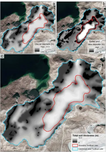
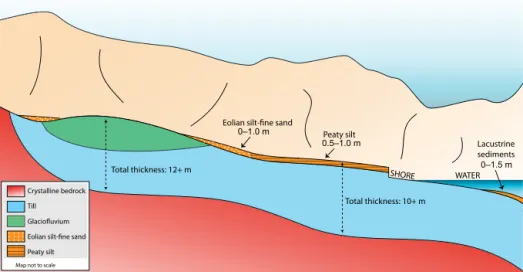
Figure 5 shows the final model of the thickness of each sediment layer. Glacial deposits (Fig. 5a), mainly till, have been deposited on top of the bedrock during periods with a more extensive Greenland Ice Sheet. At higher elevations, and where the slope is steep, no glacial deposits are generated in the model. Thinner layers of sediment are found in close proximity to exposed bedrock. In flatter terrain and in central parts of valleys, the sediment thickness increases to around 10 m. A thin layer of eolian silt covers much of the glacial deposits (Fig. 5b). These eolian deposits have a maximum depth of 1 m in flat terrain and generally decrease where the topography steepens. Figure 5b also shows the lacustrine silt at the lake floor. Lake deposits are only found at depths below 2 m in the model, and they gradually increase with depth, reaching a maximum of 1.5 m at the deepest part of the lake. The results have been used to construct a schematic sedi-ment distribution model within the catchsedi-ment (Fig. 6). Till makes up the majority of the volume of sediment and is present in all areas of the catchment. At the valley floors, the eolian silt is partly rich in organic material due to higher soil water content and is denoted peaty silt. The maximum thickness of the sediments can be found where the glacial de-posits constitute positive landforms, such as along glacioflu-vial ridges.
3.2 Active layer
Based on the methodology described in Sect. 3.2 and 3.3, a catchment-wide model of the active layer was produced (Fig. 7a). The shallowest active layer is found within the val-ley wetlands, often in close proximity to the lake and has an average maximum thickness of 0.48 m. Areas dominated by
heath,Betulaand grassland, generally constituting drier
ar-eas, have a thicker maximum active layer (between 0.68 and 0.80 m). The thickest active layer is, however, found in the barren areas with exposed bedrock (2.0 m), where the pre-defined value of 2.0 m is used (see above). The active layer depth gradually increases along the shore, where it evolves into the talik feature. The schematic figure represents a gen-eral valley area of the catchment, ranging from the catchment boundary towards the lake. There are four main valleys in the catchment area, which are marked with black dashed lines in
Figure 5.Modeled sediment thickness for different classes of
sed-iments in the catchment of Two Boat Lake.(a)Glacial deposit (till
and glaciofluvial material) thickness,(b)eolian and lake deposits, and(c)total sediment thickness including superimposed glacial, eo-lian and lake deposits.
(approxi-Total thickness: 12+ m
Total thickness: 10+ m
0–1.0 m
Eolian silt-ine sand
Peaty silt
Lacustrine sediments
0–1.5 m
SHORE WATER
0.5–1.0 m
Crystalline bedrock
Peaty silt Glaciofluvium
Eolian silt-ine sand Till
Map not to scale
Figure 6.Schematic model and presentation of the sediment thickness from the lake (right) towards higher elevations (left) in a cross section
through the valley. Sediment classes and its visual assignment are based on Fig. 3b.
mately 0.3 m) and have thus been included in the schematic model (Fig. 7b).
Based on the soil temperatures, monitored in the vegeta-tion class heath, the development of the thaw depth in the active layer can be visualized in a contour plot which cov-ers the entire period of September 2010 to December 2015 (Fig. 8). The maximum observed thaw depth in 2011 (Fig. 8), when the GPR measurements were carried out, is 0.75 m, which is within the range of the active layer depth for the
vegetation class heat calculated to 0.68±0.09 m (Table 3).
When looking at the maximum thaw depth each year, 2011 stands out as a colder period. In subsequent years the thaw depth reaches 0.8 m or more. A consistent thaw depth, deeper than 25 cm, is reached in June in all years. The plot does not
show shallow (<25 cm) temperature fluctuations but
tem-peratures in the uppermost sediments rise above 0◦C in late
April to early May (Johansson et al., 2015). In June, the air temperature is always above freezing and the thawed depth gradually migrates downward in the soil. Maximum temper-atures in the upper part of the soil occur in early August, whereas the thawed layer continues to increase in thickness until early September, although the rate slows down during August. The upper part of the active layer freezes once air
temperatures drop below 0◦C for longer periods. Large
fluc-tuations in temperatures during the October months led to periods with freezing and thawing of the upper part of the active layer at the same time as the lower boundary of the active layer migrates upwards. Data from the soil tempera-ture station show that parts of the sediments stay thawed un-til mid-October, and in warmer years, such as 2012, as far as into early November. In this way, different surface condi-tions leads to variation in not only the length of the active period, i.e., the time period when a thawed active layer ex-ists, but also the active layer thickness. The general pattern of the evolution of the active layer is similar each year: a rapid
thaw in early June which stagnates in late August followed by a more complex refreeze in late September to October.
4 Discussion
Figure 7.(a)Maximum active layer thickness over the entire catchment of Two Boat Lake with dashed ellipsoids marking valleys found within the catchment.(b)Schematic model of the variation in active layer thickness in a cross section of a valley found within the catchment
of Two Boat Lake and its relation to topography, regolith, permafrost features and surface vegetation.
2015 2014
2013 2012
2011 2010
0.25 0.50 0.75 1.00 1.25 1.50 1.75 2.00
Depth (m)
0.25 0.50 0.75 1.00 1.25 1.50 1.75 2.00 4
2 1 0 -1 -2 -4 -8
-16 °C
Figure 8.Temperature in the upper 2 m of sediments during the period of September 2010 to December 2015. Contour values are shown in
◦C, where yellow to orange gradients represent the active layer and blue gradients frozen soil.
was used with the GPR, especially when working in a large area such as the studied catchment. However, radar measure-ments can continuously map variations in active layer thick-ness in a relatively short amount of time. The result from
barren areas, often with little to no soil water content. Here we used temperature measurements from a nearby borehole, which showed the active layer extending down to 2.0 m in the bedrock (Harper et al., 2011). The significant increase in active layer thickness in the bedrock compared to sedi-ments can be explained by the difference in thermal proper-ties, namely thermal diffusivity. Bedrock has a higher diffu-sivity compared to the sediments and transfer heat at a higher rate (Janza, 1975), affecting the energy transfer from the sur-face and leading to deeper penetration of energy (heat) in a given active period. The same argument can be applied to the difference in the active layer thickness between differ-ent vegetation classes. Since the surface vegetation is directly connected to soil moisture content, differences in water con-tent of the sediments will affect the diffusivity of the
mate-rial. The diffusivity of water (1.5×10⁻³cm2s−1) compared
to that of soil (3–5×10⁻³cm2s−1) will lead to a quicker
thickening of the active layer and hence deeper permafrost table during the active period. The energy from the surface has several sources, including air temperature, precipitation and solar radiation, that will also influence the active layer thickness. This relationship has not been investigated in the present study and variations in these parameters within the catchment are not accounted for in detail. However, inves-tigations of the active layer depth have been carried out in different areas within the catchment, and local variations are therefore assumed to be included in the final model results. In this study we focus on the spatial and temporal variation in the active layer within the catchment. The permafrost bound-ary is at, or very near, its deepest point in August. However, it should be noted that the GPR measurements were carried out in 2011. This year is shown to have the shallowest observed thaw depth at the soil temperature station in the end of the active period. During the period of soil temperature measure-ments (Fig. 8), the temperature sensor at 1 m depth never
ex-perienced temperatures below 0◦C. The average thaw depth
in the active layer for the period 2011–2015 is 0.9 m. The measurements and active layer model produced here reflect the year of 2011 and should therefore perhaps be seen as a low value for the thickness of the active layer.
Long-term variations in the thawing depth or in the du-ration of the active period may affect the local hydrology and transport of matter in the catchment. An increased thaw depth of the active layer might open up new pathways for wa-ter to flow, drastically alwa-tering the subsurface hydrology of the catchment. Additionally, it is unclear whether increased thawing of the active layer will lead to drier or wetter condi-tions in Arctic landscapes, which affects the cycling of car-bon. The presented models of ALT and sediment thickness can be used as input in hydrological models aiming at inves-tigating the storage and partitioning of water in Arctic land-scapes under increased thawing conditions.
5 Data availability
All data needed to construct the soil and active layer mod-els, as well as the models themselves, are freely available from PANGAEA: doi:10.1594/PANGAEA.845258. The spa-tial information on sediment distribution with depth is valu-able when assigning hydraulic properties to conceptual and numerical hydrological models of the catchment, which in turn may be used to model biogeochemical transport and pro-cesses in both the limnic and terrestrial system.
6 Conclusion
We have used a combination of remote sensing, ground-penetrating radar, field surveys, digital elevation model anal-ysis and probe measurements to construct two models over the catchment: one of the sediment thickness and another of the maximum active layer thickness. The sediment thick-ness ranges from 0 m in bedrock outcrops areas to more than 12 m in the central valleys. The active layer is mostly con-fined within the upper 0.7 m of the sediment (excluding the bedrock), which mostly consists of eolian silt. The active layer thickness varies from 0.3 m in the wetland areas to 2 m in areas with bedrock outcrops.
model (DEM)
The digital elevation model was developed using data from three data sources:
i. an aerial photo from the company providing aerial pho-tos, Scancort;
ii. combined GPS and echo-sounding measurements in the lake to create the bathymetry;
iii. lidar data from measurements presented in the present paper.
The coverage for each data source is presented in Fig. A1. Details about the data processing based on information from Scancort are presented in Clarhäll (2011). Two mea-surement campaigns with the combined GPS–echo-sounding technique were performed: one campaign in 2010 and one in 2011. Details about the measurements performed in 2010 are presented in Clarhäll (2011), and the measurements per-formed in 2011 are described in the present paper. The GPS acquisition for the bathymetry was done without real-time kinematic correction, as there is no such option for this particular GPS receiver. The combined GPS–echo-sounding equipment (Humminbird 798ci HD SI) has estimated
accu-racy in the range of±1 m in the horizontal plane and±0.1 m
in depth.
Author contributions. Johannes Petrone prepared the manuscript
with contributions from all co-authors, performed the GPR mea-surements and the analysis of all GPR data, and established the method for upscaling the GPR data to represent the active layer thickness at catchment scale by combining them with vegetation data.
Gustav Sohlenius carried out the site investigation related to sed-iment thickness and properties, was involved in the modeling of the sediment thickness, and wrote the associated parts of the manuscript.
Emma Johansson (hydrology and meteorology) and Tobias Lind-borg (ecology and chemistry) are responsible for the GRASP field program. They were both involved in the planning of all field inves-tigations presented in this paper and were actively involved in the writing of this paper.
Mårten Strömgren wrote the parts describing the construction of the digital elevation model and was involved in the associated investi-gations.
Lars Brydsten was involved in the investigations associated with the digital elevation model.
Jens-Ove Näslund was involved in the field work and was actively involved in the writing of the paper.
Acknowledgements. The majority of the work was conducted
as a part of the Greenland Analogue Surface Project (GRASP) funded by the Swedish Nuclear Fuel and Waste Management Company (SKB). The authors would like to thank the Greenland Analogue Project (GAP) for providing additional lidar data of the catchment, and Kangerlussuaq International Science Support (KISS) for providing logistical support throughout the years.
Edited by: G. G. R. Iovine
Reviewed by: J. Engström, O. G. Terranova, and one anonymous referee
References
Burrows, M. T., Schoeman, D. S., Buckley, L. B., Moore, P., Poloczanska, E. S., Brander, K. M., Brown, C., Bruno, J. F., Duarte, C. M., Halpern, B. S., Holding, J., Kappel, C. V., Kiessling, W., O’Connor, M. I., Pandolfi, J. M., Parmesan, C., Schwing, F. B., Sydeman, W. J., and Richardson, A. J.: The pace of shifting climate in marine and terrestrial ecosystems, Science, 334, 652–655, doi:10.1126/science.1210288, 2011.
Cappelen, J. (Ed.): Weather and climate data from Greenland 1958– 2013 – Observation data with description, DMI Technical Report 14-08, Copenhagen, 2014.
Christiansen, H. and Humlum, O.: Permafrost, in: Topografisk Atlas Grönland, edited by: Jakobsen, B. H., Böcher, J., Nielsen, N., Guttesen, R., Humlum, and O., Jensen, E., Det Kongelige Danske Geografiske Selskab/Kort & Matrikelstyrelsen, 32–35, 2000. Clarhäll, A.: SKB studies of the periglacial environment – report
from field studies in Kangerlussuaq, Greenland 2008 and 2010, SKB P-11-05, Swedish Nuclear Fuel and Waste Management Co., 2011.
Davis, J. C.: Statistics and Data Analysis in Geology, John Wiley and Sons: New York, 1986.
Doolitle, J. A., Hardisky, M. A., and Gross, M. F.: A groundpene-trating radar study of the active layer thickness in areas of moist sedge and wet sedge tundra near Bethel, Alaska, U.S.A., Arctic Alpine Res., 22, 175–182, doi:10.2307/1551302, 1990. Ermakov, A. P. and Starovoitov, A. V.: The use of the
ground penetrating radar (gpr) method in engineering-geological studies for the assessment of geological-cryological condi-tions, Moscow University Geology Bulletin, 65, 422–427, doi:10.3103/S0145875210060116, 2010.
Gacitúa, G., Tamstorf, M. P., Kristiansen, S. M., and Uribe, J. A.: Estimations of moisture content in the active layer in an arctic ecosystem by using ground-penetrating radar profiling, J. Appl. Geophys., 79, 100–106, doi:10.1016/j.jappgeo.2011.12.003, 2012.
Harper, J., Hubbard, A., Ruskeeniemi, T., Claesson Liljedahl, L., Lehtinen, A., Booth, A., Brinkerhoff, D., Drake, H., Dow, C., Doyle, S., Engström, J., Fitzpatrik, A., Frape, S., Henkemans, E., Humphrey, N., Johnson, J., Jones, G., Joughin, I., Klint, K. E., Kukkonen, I., Kulessa, B., Londowski, C., Lindbäck, K., Makah-nouk, M., Meierbachtol, T., Pere, T.,Pedersen, K., Petterson, R., Pimentel, S., Quincey, D., Tullborg, E. L., and van As, D.: The Greenland Analogue Project Yearly Report 2010. Svensk Kärn-bränslehantering AB, Report SKB R-11-23, 2011.
Isaaks, E. H. and Srivastava, R. M.: An introduction to applied geo-statistics, Oxford University Press: Oxford, 1989.
Janza, F. J.: Interaction mechanisms, in: Manual of remote sensing, edited by: Reeves, R. G., Anson, A., and Landen, D., American Society of Photogrammetry: Falls Church, VA, 75–179, 1975. Johansson, E., Berglund, S., Lindborg, T., Petrone, J., van As, D.,
Gustafsson, L.-G., Näslund, J.-O., and Laudon, H.: Hydrologi-cal and meteorologiHydrologi-cal investigations in a periglacial lake catch-ment near Kangerlussuaq, west Greenland – presentation of a new multi-parameter data set, Earth Syst. Sci. Data, 7, 93–108, doi:10.5194/essd-7-93-2015, 2015.
Jørgensen, A. and Andreasen, F.: Mapping of permafrost sur-face using ground-penetrating radar at kangerlussuaq airport, Western Greenland, Cold Reg. Sci. Technol., 48, 64–72, doi:10.1016/j.coldregions.2006.10.007, 2007.
Larsen, J. N., Anisimov, O. A., Constable, A., Hollowed, A. B., Maynard, N., Prestrud, P., Prowse, T. D., and Stone, J. M. R.: Po-lar regions, in: Climate Change 2014: Impacts, Adaptation, and Vulnerability. Part B: Regional Aspects. Contribution of Working Group II to the Fifth Assessment Report of the Intergovernmen-tal Panel on Climate Change, edited by: Barros, V. R., Field, C. B., Dokken, D. J., Mastrandrea, M. D., Mach, K. J., Bilir, T. E., Chatterjee, M., Ebi, K. L., Estrada, Y. O., Genova, R. C., Girma, B., Kissel, E. S., Levy, A. N., MacCracken, S., Mastrandrea, P. R., and White, L. L., Cambridge University Press, Cambridge, United Kingdom and New York, NY, USA, 1567–1612, 2014. Lindborg, T., Rydberg, J., Tröjbom, M., Berglund, S., Johansson,
E., Löfgren, A., Saetre, P., Nordén, S., Sohlenius, G., Anders-son, E., Petrone, J., Borgiel, M., Kautsky, U., and Laudon, H.: Biogeochemical data from terrestrial and aquatic ecosystems in a periglacial catchment, West Greenland, Earth Syst. Sci. Data, 8, 439–459, doi:10.5194/essd-8-439-2016, 2016.
principles, problems and progress, Earth-Sci. Rev., 66, 261–330, doi:10.1016/j.earscirev.2004.01.004, 2004.
Nelson, F. E. and Anisimov, O. A.: Permafrost zonation in Rus-sia under anthropogenic climate change, Pemafrost Periglac., 4, 137–148, doi:10.1002/ppp.3430040206, 1993.
MacCraken, M. C., Hecht, A. D., Budyko, M. I., and Izrael, Y. A.: Prospects for Future Climate: A special US/USSR Report on Climate and Climate Change, Lewis Publishers: Chelsea, Mich., 1990.
Macdonald, R. W., Harner, T., and Fyfe, J.: Recent climate change in the Arctic and its impact on contaminant pathways and inter-pretation of temporal trend data, Sci. Total Environ., 342, 5–86, doi:10.1016/j.scitotenv.2004.12.059, 2005.
Maxwell, J. B. and Barrie, L. A.: Atmospheric and climatic change in the Arctic and Antarctic, Ambio, 18, 42–49, 1989.
Pastick, N. J, Jorgenson, M. T., Wylie, B. K., Minsley, B. J., Ji, L., Walvoord, M. A., Smith, B. D., Abraham, J. D., and Rose, J. R.: Extending Airborne Electromagnetic Surveys for Regional Active Layer and Permafrost Mapping with Remote Sensing and Ancillary Data, Yukon Flats Ecoregion, Central Alaska, Per-mafrost Periglac., 24, 184–199, doi:10.1002/ppp.1775, 2013. Petrone, J.: Using ground-penetrating radar to estimate sediment
load in and around Two BoatLake, western Greenland, Student thesis, Uppsala universitet, Uppsala, available at: http://urn.kb. se/resolve?urn=urn:nbn:se:uu:diva-196291 (last access: 2016), 2013.
Roots, E. F.: Climate change: high latitude regions, Climatic Change, 15, 223–253, doi:10.1007/BF00138853, 1989.
Harden, J. W., Hayes, D. J., Hugelius, G., Koven, C. D., Kuhry, P.,Lawrence, D. M., Natali, S. M., Olefeldt, D., Romanovsky, V. E., Schaefer, K., Turetsky, M. R., Treat, C. C., and Vonk, J. E.: Climate change and the permafrost carbon feedback, Nature, 250, 171–178, 2015.
Stevens, C. W., Moorman, B. J., Solomon, S. M., and Hugenholtz, C. H.: Mapping subsurface conditions within the near-shore zone of arctic delta using ground penetrating radar, Cold Reg. Sci. Technol., 56, 30–38, doi:10.1016/j.coldregions.2008.09.005, 2009.
van Tatenhove, F., van der Meer, J., and Koster, E.: Implications for deglaciation chronology from new AMS age determina-tions in central west Greenland, Quaternary Res., 45, 245–253, doi:10.1006/qres.1996.0025, 1996.
Walter, K. M., Zimov, S. A., Chanton, J. P., Verbyla, D., and Chapin, F. S.: Methane bubbling from Siberian thaw lakes as a positive feedback to climate warming, Nature, 443, 71–75, 2006. Weller, G., Chapin, F. S., Everett, K. R., Hobbie, J. E., Kane, D.,
Oechel, W. C., Ping, C. L., Reeburgh, W. S., Walker, D., and Walsh, J.: The Arctic Flux Study: a regional view of trace gas release, J. Biogeogr., 22, 365–374, doi:10.2307/2845932, 1995. Willemse, N. W., Koster, E. A., Hoogakker, B., and van
Taten-hove, F. G. M.: A continous record of Holocene eolian ac-tivity in Western Greenland, Quaternary Res., 59, 322–334, doi:10.1016/S0033-5894(03)00037-1, 2003.