www.the-cryosphere.net/10/2573/2016/ doi:10.5194/tc-10-2573-2016
© Author(s) 2016. CC Attribution 3.0 License.
Seasonal evolution of the effective thermal conductivity of the snow
and the soil in high Arctic herb tundra at Bylot Island, Canada
Florent Domine1,2,3,4, Mathieu Barrere1,3,4,5,6, and Denis Sarrazin3
1Takuvik Joint International Laboratory, Université Laval (Canada) and CNRS-INSU (France), Pavillon Alexandre Vachon,
1045 Avenue de la Médecine, Québec City, QC, Canada
2Department of Chemistry, Université Laval, Québec City, QC, Canada 3Centre d’Études Nordiques, Université Laval, Québec City, QC, Canada 4Department of Geography, Université Laval, Québec City, QC, Canada 5Météo-France – CNRS, CNRM UMR 3589, CEN, Grenoble, France 6LGGE, CNRS-UJF, Grenoble, France
Correspondence to:Florent Domine ([email protected])
Received: 3 May 2016 – Published in The Cryosphere Discuss.: 13 May 2016
Revised: 6 October 2016 – Accepted: 12 October 2016 – Published: 2 November 2016
Abstract. The values of the snow and soil thermal conduc-tivity, ksnow and ksoil, strongly impact the thermal regime
of the ground in the Arctic, but very few data are avail-able to test model predictions for these variavail-ables. We have monitoredksnowandksoilusing heated needle probes at
By-lot Island in the Canadian High Arctic (73◦N, 80◦W)
be-tween July 2013 and July 2015. Few ksnow data were ob-tained during the 2013–2014 winter, because little snow was present. During the 2014–2015 winter ksnow monitor-ing at 2, 12 and 22 cm heights and field observations show that a depth hoar layer with ksnowaround 0.02 W m−1K−1 rapidly formed. At 12 and 22 cm, wind slabs with ksnow
around 0.2 to 0.3 W m−1K−1 formed. The monitoring of ksoil at 10 cm depth shows that in thawed soil ksoil was
around 0.7 W m−1K−1, while in frozen soil it was around
1.9 W m−1K−1. The transition between both values took
place within a few days, with faster thawing than freezing and a hysteresis effect evidenced in the thermal conductivity– liquid water content relationship. The fast transitions sug-gest that the use of a bimodal distribution ofksoil for
mod-elling may be an interesting option that deserves further test-ing. Simulations ofksnowusing the snow physics model Cro-cus were performed. Contrary to observations, CroCro-cus pre-dicts high ksnowvalues at the base of the snowpack (0.12– 0.27 W m−1K−1) and low ones in its upper parts (0.02–
0.12 W m−1K−1). We diagnose that this is because
Cro-cus does not describe the large upward water vapour fluxes
caused by the temperature gradient in the snow and soil. These fluxes produce mass transfer between the soil and lower snow layers to the upper snow layers and the atmo-sphere. Finally, we discuss the importance of the structure and properties of the Arctic snowpack on subnivean life, as species such as lemmings live under the snow most of the year and must travel in the lower snow layer in search of food.
1 Introduction
Arctic permafrost contains large amounts of frozen organic matter (Hugelius et al., 2014). Its thawing could lead to the microbial mineralisation of a fraction of this carbon, result-ing in the release of yet undetermined but potentially very important amounts of greenhouse gases (CO2 and CH4) to
particu-lar is often mentioned as a key factor in the permafrost ther-mal regime (Gouttevin et al., 2012; Burke et al., 2013). How-ever, most land surface models which use an elaborate snow scheme often simply parameterise snow thermal conductiv-ity as a non-linear function of its densconductiv-ity. Even though the average density of snow may be adequately predicted in land surface models (Brun et al., 2013), the density profile of Arc-tic or subarcArc-tic snow is currently not predicted well by most or all snow schemes (Domine et al., 2013) because the up-ward water vapour flux generated by the strong temperature gradients present in these cold snowpacks (Sturm and Ben-son, 1997) is not taken into account. These fluxes lead to a mass transfer from the lower to the upper snow layers, and these transfers can result in density changes of 100 kg m−3,
perhaps even more (Sturm and Benson, 1997; Domine et al., 2013). Given the non-linearity between snow thermal con-ductivity and density used in most snow schemes, errors in the snow density vertical profile inevitably lead to errors in the snowpack thermal properties and therefore in the per-mafrost thermal regime.
Obviously, soil thermal conductivity is also important in determining vertical heat fluxes. For a given soil composi-tion, this variable depends mainly on temperature and tent in liquid water and ice, so that its value may show con-siderable variations over time (Penner et al., 1975; Overduin et al., 2006). Modellers of the permafrost thermal regime have stressed that “monitoring of this parameter in the ac-tive layer all year-round would be useful if a more realistic numerical model is to be developed” (Buteau et al., 2004).
Another important interest of studying snow physical properties such as thermal conductivity and the heat budget of the ground lies in the understanding of the conditions for subnivean life. For example, lemmings live under the snow most of the year at Bylot Island (Bilodeau et al., 2013), and the temperature at the base of the snowpack conditions their energy expenses to maintain body temperature. Furthermore, energy expense for subnivean travel in search of food de-pends on snow hardness and snow conditions have been in-voked to help explain lemming population cycles (Kausrud et al., 2008; Bilodeau et al., 2013), even though no compre-hensive snow studies have yet been performed to fully es-tablish links between lemming populations and snow prop-erties. Snow thermal conductivity has been shown to be well correlated with snow mechanical properties (Domine et al., 2011), so that monitoring snow thermal conductivity may help quantify the effort required by lemmings to access food and hence understand their population dynamics.
Given the importance of snow thermal conductivity to sim-ulate the ground thermal regime and to understand the con-ditions for subnivean life, we have initiated continuous auto-matic measurements of the snow thermal conductivity verti-cal profile at several Arctic sites using heated needle probes (NPs). The first instrumented site was in low Arctic shrub tundra (Domine et al., 2015), near Umiujaq on the eastern shore of Hudson Bay. We present here an additional study
with 2 years of snow thermal conductivity monitoring at By-lot Island, a high Arctic herb tundra site (73◦N, 80◦W).
Since lemming populations have been monitored there for over 2 decades (Bilodeau et al., 2013; Fauteux et al., 2015), the snow work undertaken here may indeed also help un-derstand snow–lemming relationships. Additionally, we also placed a heated NP in the soil at a depth of 10 cm to monitor soil thermal conductivity in the active layer over the seasonal freeze–thaw cycles.
2 Methods
2.1 Study site and instrumentation
Our study site is on Bylot Island, just north of Baffin Island in the Canadian high Arctic. The actual site was at the bot-tom of Qalikturvik valley, in an area of ice-wedge polygons (73◦09′01.4′′N, 80◦00′16.6′′W), in a context of high Arctic
thick permafrost. This spot is within 100 m of that described by Fortier and Allard (2005). Our instruments were placed in July 2013 in a fairly well-drained low-centre polygon with peaty silt soil (Fig. 1). Vegetation consists of sedges, graminoids and mosses (Bilodeau et al., 2013). The active layer is about 30 cm deep at our site and permafrost at Bylot Island is thought to be several hundred metres deep (Fortier and Allard, 2005). The site is only accessible with complex logistics, so that field work only takes place in late spring and summer.
rel-Figure 1.Location of the study site on Bylot Island in the Canadian Arctic archipelago and photograph of the monitoring station deployed.
The polyethylene post with the three TP08 heated needle probes is in the foreground. The polyethylene post with the five thermistors is visible behind it. The radiometers, SR50 snow height gauge, cup anemometer, temperature and relative humidity gauge, and surface temperature sensors are visible on the tripod, from left to right. The CR1000 data loggers and batteries are in the metal box on the tripod. Batteries are recharged by solar panels and a wind mill in winter. Inset: detail of the lower two TP08 needles after their positions were lowered in July 2014.
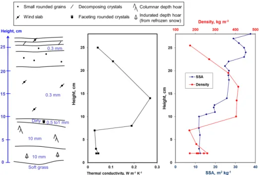
Figure 2.Stratigraphy and vertical profiles of snow physical properties near our study site on 12 May 2015. Visual grain sizes are indicated
in the stratigraphy. Density data are for the middle of the 3 cm high sample. Snow type symbols are those of Fierz et al. (2009), except for the basal melt–freeze layer, which transformed into depth hoar to form an indurated layer, as detailed in the text.
ative humidity with a HC2S3 sensor from Rotronic and wind speed with a cup anemometer, both at 2.3 m height, and snow height with an SR50A acoustic snow height gauge (Camp-bell Scientific), an IR120 infrared surface temperature sensor and a CNR4 radiometer with a CNF4 heating/ventilating sys-tem from Kipp & Zonen which measured downwelling and upwelling short-wave and long-wave radiation. Heating and
measurements were recorded, except for the TP08 needles, whose operation is described in the next section.
2.2 Thermal conductivity measurements
The NP method has been used extensively for soils for a long time (Devries, 1952). Sturm and Johnson (1992) and Morin et al. (2010) discussed in detail the heated NP method in snow. The automatic operation of the TP08 needles in Arctic snow and the data analysis have been detailed in Domine et al. (2015) and only a brief summary will be given here.
For a measurement cycle, the 10 cm long needles were heated at constant power (0.4 W m−1) for 150 s. The
temper-ature was monitored by a thermocouple at the centre of the heated zone. Heat loss is a function of the thermal conduc-tivity of the medium. A plot of the thermocouple temperature as a function of ln(t), wheret is time, theoretically yields a linear curve after an initiation period of 10 to 20 s. The slope of the linear part is inversely proportional to the thermal con-ductivity of the medium.
In snow, NPs in fact measure an effective thermal conduc-tivity,ksnow, with contributions from conductive heat
trans-fer through the network of interconnected ice crystals and through the interstitial air, as well as heat transfer due to latent heat exchanges caused by water molecules sublima-tion and condensasublima-tion generated by the temperature gradi-ent around the heated NP (Sturm et al., 1997; Calonne et al., 2011). The variableksnowis defined as
F = −ksnowdT
dz, (1)
with dT /dz the vertical temperature gradient through the layer, in K m−1, andF the heat flux in W m−2.
The automatic routine developed by Domine et al. (2015) was used to obtain ksnow from the heating curve. Essen-tially, that routine detects possible non-linearity in the heat-ing curve and selects the most linear curve section to de-termine ksnow. The main cause of non-linearity is the
oc-currence of convection in the snow, which, by adding an extra heat transfer process, reduces the rate of temperature rise. This readily happens in depth hoar after 50 to 60 s of heating because of its high permeability. Since convective heat transfer is not an intrinsic snow property because it de-pends, among other things, on the heating power, it has to be detected and data affected by it must be discarded. There-fore, while the 40–100 s heating time range was used to de-rive ksnow for heating curves not perturbed by convection, the range 20–50 s was used when convection was present (Domine et al., 2015). Other causes of non-linearity include non-homogeneous snow and melting due to excessive heat-ing. To avoid melting, automatic measurements were started only if the snow temperature was <−2◦C. Factors such as
non-homogeneous snow may result in poor-quality heating curves, which were discarded. Thermal conductivity mea-surements were performed once every 2 days to take into
account the slow evolution of this variable and to minimise thermal perturbation to the snow. Measurements were per-formed at 05:00 to minimise the risk of having warm snow. The NP heating sequence takes place regardless of whether the NP is covered by snow or not. Theksnowdata that we de-termined took place in air were discarded. When an NP is not snow covered, even a slight wind produces an erratic heating curve. Should there be very little wind, snow height measure-ment, the value ofksnowand the presence of convection often
allow the detection of a non-covered probe. Incorrect or un-certain determination of NP snow coverage is nevertheless still possible, and this will be discussed when relevant.
Measurements of soil thermal conductivityksoil were not
performed by Domine et al. (2015), and details are therefore given here. Since snow and soil NPs are all multiplexed onto the same data logger, the same heating power had to be used in snow and soil. The thermal conductivity of soils, espe-cially when frozen, can be much greater than that of snow (Penner, 1970), so that heating by the NP can be much lower, resulting in more noise in the heating curves. NPs do not in-duce convection in soils because of their low permeability, so that heating curves were always linear. The 30–90 s heating time range was thus used. A quality threshold based on the determination coefficient of the curve was used and curves withR2< 0.75 were discarded.
Measuring thermal conductivity in porous granular media such as snow has been suspected of presenting biases and/or systematic errors (Calonne et al., 2011; Riche and Schnee-beli, 2013) and these have been discussed by Domine et al. (2015). One concern is that the relevant metric for heat ex-changes between the ground and the atmosphere through the snow is the vertical heat flux. Snow is anisotropic (Calonne et al., 2011; Riche and Schneebeli, 2013) and NPs measure a mixture of vertical and horizontal heat fluxes. Anisotropy depends on snow type, with, for example, depth hoar being more conductive in the vertical direction and wind slabs in the horizontal direction. Moreover, a systematic error caused by the granular nature of snow was invoked by Riche and Schneebeli (2013). Domine et al. (2015) discussed the im-pact of these processes on the accuracy ofksnow
measure-ment with NPs and concluded that if the snow type was not known, the maximum error was typically 29 %. The largest contributions to error were the systematic error due to the use of the NP (20 %) and error due to anisotropy (20 %). The total error is the square root of the sum of the squares of all contributions. If the snow type is known, corrections for anisotropy and systematic bias are possible, potentially re-ducing errors to 10 to 20 %. Such corrections were not, how-ever, performed by Domine et al. (2015). Given thatksnow varies between 0.025 and 0.7 W m−1K−1, errors due to the
use of NPs are quite acceptable and measurements using NPs still very useful. Alternativeksnowmeasurement methods, i.e.
high Arctic sites because they require sampling and complex instruments.
For soils, the issues raised by Riche and Schneebeli (2013) are expected to have no impact because soils are much denser with smaller grains and are closer to a homogeneous medium at the scale of a NP. Anisotropy may, however, be an issue in some soil types, but we have not developed this aspect here. Based on the quality of our soil heating curves, we estimate that the error on ksoil is 15 % or less when the soil is not
frozen and 25 % when it is frozen, because higherksoilmeans
lower heating by the NP and therefore less accurate heating curves.
Field measurements of snowksnowand soilksoilwere also
performed during field campaigns in spring 2014 and 2015 and summer 2013, 2014 and 2015 with a TP02 NP. Addi-tional spring field measurements included snow density with a 100 cm3, 3 cm high box cutter, which has a typical error
of 10 %, snow temperature, and snow-specific surface area (SSA) with the DUFISSS instrument based on infrared re-flectance at 1310 nm (Gallet et al., 2009). SSA is the surface area per mass and is thus inversely proportional to snow grain size. SSA can be used to evaluate the intensity of metamor-phism, as intense metamorphism driven by high temperature gradients lead to rapid grain growth and hence SSA decrease (Taillandier et al., 2007). The error on SSA is 12 % (Gallet et al., 2009). Some of these snow measurements have been detailed by Domine et al. (2016). Additional summer mea-surement included soil volume water content using an EC5 sensor from Decagon.
2.3 Soil granulometric analysis
Soil grain size distribution is useful to understand its physical properties. Samples were taken from our instrumented site at 10 cm depth in July 2015. Particle size distribution was measured with a Horiba partica LA-950V2 laser scattering particle size analyser, which used a two-wavelength optical system, 405 and 650 nm. Five subsamples were analysed and averaged.
2.4 Snow physics modelling
We used the Crocus model (Vionnet et al., 2012) coupled to the land surface model ISBA within the SURFEX inter-face (version 7.3) to simulate snow physical properties. We in fact used the simulations already described in Domine et al. (2016) for our Bylot Island site, but we analysed different output data. Very briefly, the model was forced with our me-teorological data. When data were missing, ERA-Interim re-analysis data were used (Dee et al., 2011), corrected follow-ing the procedure of Vuichard and Papale (2015) to minimise the bias between measured and ERA data. Snow thermal con-ductivity is calculated from the equation of Yen (1981), based on a correlation between density and thermal conductivity.
3 Results
The winter 2013–2014 was a low snow year so that two out of three NPs were not covered. Data are more complete for the following year and we therefore start with data from the 2014–2015 season.
3.1 2014–2015 season
Describing the structure and physical properties of the snow-pack at Bylot Island helps to understand the monitoring data. Observations made on 12 May 2015 close to our monitor-ing site are shown in Fig. 2. Vegetation was observed to be mostly flattened by snow, with some sedge or graminoids stems still upright, but they did not seem to have impacted snow structure. We observed a basal depth hoar layer 8 to 10 cm thick, overlaid by a wind slab 11 to 12 cm thick, with in-between a thin layer of faceting crystals. Above the wind slab were thin layers of small rounded grains, decompos-ing precipitation crystals and a thin wind crust. The depth hoar layer was divided into two sublayers. The lower sub-layer was slightly indurated and harder, although hardness and other properties appeared spatially very variable. In-durated depth hoar is a snow type seldom mentioned, as it does not form in alpine or temperate snow, and it is not de-scribed in the international snow classification (Fierz et al., 2009) despite its widespread presence in the Arctic, where it has been observed without being named for decades. Hall et al. (1991) described “solid-type depth hoar”, presumably indurated depth hoar. Sturm et al. (2002) mentioned “wind slab to depth hoar” layers, presumably also indurated depth hoar. Its most detailed description is probably that of Sturm et al. (2008):
This type of layer is generally not seen outside of the Arctic. It arises in the Arctic because the tem-perature gradients are so strong that even dense, fine-grained layers of wind slab eventually meta-morphose into large, faceted, and striated depth hoar grains. A key characteristic of these slab-to-hoar layers is that they are tough, not fragile like most depth hoar. If comprised of mainly depth hoar crystals, yet still cohesive, we called the layers “in-durated”. If a significant number of small wind grains remained, we called them “slab-like”. Domine et al. (2016) gave complementary details:
Indurated depth hoar . . . forms in dense wind slabs under very high temperature gradients not en-countered in alpine snow. Its density can exceed 400 kg m−3. Large depth hoar crystals coexist with
depth hoar . . . ) which has a very low cohesion, indurated depth hoar is reasonably cohesive, al-though fairly brittle, and large blocks can easily be cut out of it and manipulated.
The indurated depth hoar here showed signs of early sea-son melting in the form of rounded grains that were partially to almost totally transformed into depth hoar, but bonds were stronger than for regular depth hoar. There are therefore two main precursors to indurated depth hoar: wind slabs as de-tailed by Sturm et al. (2008) and refrozen layers as observed here and to the best of our knowledge only previously de-scribed in Domine et al. (2016). The indurated depth hoar that forms in refrozen snow is slightly different from that observed in wind slabs, in that no small grains are present and it does not have a milky aspect. In line with Domine et al. (2016), we represent this type of depth hoar with a symbol that does not exist in the classification of Fierz et al. (2009), as that classification is ideal for alpine snow but is not detailed enough to represent many Arctic snow types. The depth hoar upper sublayer was very soft, appeared more homogeneous and showed no signs of melting. Vertical pro-files of density, SSA and thermal conductivity are also shown in Fig. 2. Several density measurements were made in the lower depth hoar layer, yielding values between 172 and 260 kg m−3. In comparison, the upper depth hoar layer was
at 170 kg m−3, a rather low value for depth hoar. The
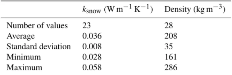
verti-cal profiles of the three measured physiverti-cal variables reflect the observed stratigraphy rather well, with higher values of all three variables for the wind slab and lower values for the depth hoar, as already noted by Domine et al. (2016). The basal snow temperature was−17.1◦C. Despite spatial variations in snow height and layer thickness, the profiles of Fig. 2 are fairly typical. We measured 10 such profiles on herb tundra. In particular, the values ofksnowand density in the basal depth hoar layer seemed to all be within a fairly narrow range, as detailed in Table 1.
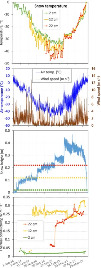
Figure 3 shows time series forksnow, as well as snow
tem-perature, air temtem-perature, wind speed and snow height. Snow height is spatially very variable in the Arctic at the 50 cm scale, mostly because of wind effects and of microtopogra-phy. Typically, in May around our site, snow height varied between 22 and 45 cm within 5 m. Measurements using an avalanche probe at 236 spots within 200 m of our site on 12 May 2015 showed a mean snow height of 25.3 cm, with a standard deviation of 13.1 cm (Domine et al., 2016). There-fore, snow height given by our acoustic snow gauge can only be taken as an indication of the actual snow height at the very NP site, about 5 m away. On 12 May 2015, snow height was 27 cm at the pit shown in Fig. 2, 50 cm from the NP post, while the snow gauge indicated 35 cm.
The lowest NP, at 2 cm, was covered by the first snow-fall on 12 September 2014. That initial snow partially melted and the first data point that was almost certainly obtained in snow was on 24 September. After initial
val-Table 1.Variations in values of thermal conductivity,ksnow, and
density of the basal depth hoar layer (lowest 5 cm) based on mea-surements in 10 pits on herb tundra.
ksnow(W m−1K−1) Density (kg m−3)
Number of values 23 28
Average 0.036 208
Standard deviation 0.008 35
Minimum 0.028 161
Maximum 0.058 286
ues around 0.04 W m−1K−1,ksnowdropped to values around
0.02 W m−1K−1 because of rapid depth hoar formation.
These values may seem a bit low, especially considering that air has a thermal conductivity of 0.023 W m−1K−1, but the
low value can be attributed to a negative systematic error of about 20 % caused by the NP method and to anisotropy as described in Riche and Schneebeli (2013) and discussed above. Indeed, depth hoar is very anisotropic and its verti-cal component has the highest value (Riche and Schneebeli, 2013). Our NP measured a mixture of vertical and horizontal components producing another negative artefact. Taking into account all error sources, the actual vertical component is probably 25 to 30 % greater than measured here, i.e. around 0.025 W m−1K−1.
The NP at 12 cm was probably in fresh snow on 1 Novem-ber. On 10 to 11 November, the strongest wind storm of the winter, reaching a speed of 12.9 m s−1, appears to have
formed a wind slab that buried the 12 cm NP, withksnow= 0.28 W m−1K−1.ksnowremained close to that value until 28
March. Until 1 January, data are noisy, possibly because the NP was close to the snow surface and therefore subject to air advection by wind, which, by adding a heat loss process, pro-duced randomly a slight positive artifact.ksnowthen dropped
to 0.23 W m−1K−1on 30 March, while no special
meteoro-logical event was recorded. Between 27 and 30 March, the wind remained under 4 m s−1 and the temperature showed
regular diurnal cycles between−40 and−20◦C. The value
ofksnowstarted rising steadily on 5 May to reach a value of
0.33 W m−1K−1on 29 May. Considerations of the evolution
of metamorphic conditions in the snowpack, discussed sub-sequently, are required to explain this process.
The NP at 22 cm was definitely covered by snow on 21 January 2015. ksnow remained around 0.06 W m−1K−1
until 8 February, indicating that it remained as undis-turbed precipitation. On that date, a moderate wind storm started, reaching 5.6 m s−1at 11:00 EST. The resulting wind
slab had ksnow=0.175 W m−1K−1, increasing steadily to 0.25 W m−1K−1 on 23 April, most likely because of slow
sintering. On 25 April, the value rose to 0.309 W m−1K−1,
Figure 3. Snow temperature, air temperature, wind speed, snow
height and snow thermal conductivity at three heights during the 2014–2015 winter season at Bylot Island. The levels of the three thermal conductivity needle probes (NPs) are indicated in the snow height panel. Note that the snow height gauge and the NPs were about 5 m away, so that snow height between both spots may have been different. Snow temperatures were measured with the NPs ev-ery other day at 05:00.
Figure 4.Vertical profiles of soil physical variables in pits dug in the polygon where our instrument station is located, during summers 2013 to 2015.(a)Temperature;(b)thermal conductivity;(c) volu-metric liquid water content.
Figure 5.Seasonal evolution of the thermal conductivity, temper-ature and volume water content of the soil at 10 cm depth for the 2014–2015 season. The 5TM probe which measures both tempera-ture and water content hourly is about 2 m from the TP08 NP, which measures thermal conductivity and temperature every 2 days.
ksnow stabilised around 0.26 W m−1K−1 until the end of
May, which we will discuss subsequently in light of meta-morphic conditions.
Three soil pits were dug in the summers 2013 to 2015 down to the thaw front in the polygon where our instruments are located to measure soil physical properties and another two pits were dug just for observations. An organic litter layer 3.5 to 6 cm thick was observed. Lower down was a layer of organic-rich silt-looking material. Figure 4 shows vertical profile of soil temperature, thermal conductivity, ksoil, and volume water content fraction. The general trend is an in-crease ofksoil with depth, while temperature expectedly de-creases. Soil grain size distribution was obtained from 5 sam-ples taken around 10 cm depth. The average data show a bi-modal size distribution with modes centred at 17 and 59 µm. If the standard 50 µm size limit between sand and silt is used, then our sample is 65 % silt and 35 % sand by mass, so that the soil here is a mixture of silt and fine sand.
Figure 5 shows the evolution of theksoil and temperature
28 July 2014 and 26 June 2015. Figure 5 also shows hourly soil temperature and volume water content at 10 cm depth measured by a 5TM probe located about 1 m away. Both temperature measurements show similar variations, but the 5TM is 1 to 2◦C warmer, in part due to a positive 0.5◦C
offset on the 5TM. The soil temperature reached 0◦C on
9 September and stayed at that temperature without signif-icant freezing, as indicated by the water content, until 27 September. The soil water freezing continued until 10 Oc-tober, at which point only water in small pores remained liquid. Until 30 September 2014, the soil thermal conduc-tivity stayed constant with ksoil=0.73 W m−1K−1, with a standard deviation of 0.02 W m−1K−1, while the soil
vol-ume water content was 49.5±1.3 %. Except for very low water contents, soil freezing is expected to manifest itself in an increase inksoil, (Penner, 1970; Inaba, 1983) because ice has a much higher thermal conductivity than water (2.22 vs. 0.56 W m−1K−1 at 0◦C). Measurements of ksoil show
de-tectable soil freezing between 30 September and 2 October, withksoilincreasing from 0.76 to 1.16 W m−1K−1. The value of ksoil then rapidly increased to 1.8 W m−1K−1on 10
Oc-tober, confirming 5TM data that the soil was then almost essentially frozen at 10 cm depth, except for water in small pores (Penner, 1970; Inaba, 1983). The average and standard deviation ofksoil then were 1.95±0.20 W m−1K−1for the winter season. The large standard deviation only indicates the greater uncertainty of our instrument for high ksoil
val-ues, because NP heating is less pronounced. Theksoilvalues
of both unfrozen and frozen soil are consistent with those expected from a fine grain mineral material mixed with or-ganic matter (Penner, 1970; Kujala et al., 2008). Even as the soil temperature decreases to−30◦C, no further increase in ksoilis observed, suggesting that essentially all the water that could was already frozen on 10 October. The value of ksoil then decreased in just a few days when thawing took place on 20 June 2015 andksoilreturned to its previous thawed value.
Figure 5 shows that the increase inksoil upon freezing takes
place at the initiation of freezing, i.e. at low ice content. In contrast, in spring the decrease inksoiltakes place at the
ini-tiation of thawing, i.e. at high ice content. There is therefore a hysteresis loop betweenksoiland water content.
3.2 2013–2014 season
Figure 6 shows the value ofksnowat a height of 7 cm for the
2013–2014 season, as only that NP was sufficiently covered to give reliable data. As previously, we also show snow tem-perature and height, wind speed and air temtem-perature. That season, the snow height at our snow gauge was noticeably lower than at our NP post. On 14 May 2014, the gauge in-dicated 13 cm, while there was 18 cm of snow at the NP post. Measurements using an avalanche probe at 314 spots within 200 m of our site on 14 May 2015 showed a mean snow height of 16.2 cm, with a standard deviation of 13.7 cm (Domine et al., 2016).
Figure 6.Snow temperature, air temperature, wind speed, snow
height and snow thermal conductivity at 7 cm height during the 2013–2014 winter season at Bylot Island. The levels of the three thermal conductivity needle probes (NPs) are indicated in the snow height panel, showing that only the lowermost NP was covered.
Figure 7.Stratigraphy and vertical profiles of snow physical properties near our study site on 14 May 2014. Fresh snow is just a 2 mm thick
sprinkling, also visible in the SSA profile. Density data are for the middle of the 3 cm high sample. Snow type symbols are those of Fierz et al. (2009), except for the lower wind slab, which transformed into depth hoar to form an indurated layer, as detailed in the text. Red-filled black squares in the stratigraphy indicate where thermal conductivity measurements were made.
Figure 8.Gaps in the snow in the basal depth hoar layer.(a, b)Gaps
due to the spontaneous collapse of the depth hoar, following season-long mass loss because of the upward water vapour flux.(c, d)
Lem-ming burrows, easily identifiable by their regular shape and the pres-ence of characteristic feces (c, foreground).
other observations, it was definitely < 200 kg m−3and more
likely around 150 kg m−3, perhaps even less. Gaps in the
basal layer were frequent, indicating that it had collapsed nat-urally in many places. These spontaneous collapse features cannot be mistaken for lemming burrows (Fig. 8). This very
soft and fragile structure was most likely due to the loss of matter caused by the upward water vapour flux generated by the temperature gradient in the snowpack. Such basal depth hoar collapse in the low and high Arctic have already been described by Domine et al. (2015, 2016). Above the basal depth hoar was a layer of indurated depth hoar formed by the metamorphism of a hard wind slab into depth hoar, as de-tailed above. Although brittle, the indurated depth hoar ob-served was fairly solid and could readily be sampled with-out damaging its structure. It has a high thermal conductiv-ity (0.37 W m−1K−1), high density (383 kg m−3) and a SSA
(14.6 to 19.6 m2kg−1) slightly lower than most wind slabs
but higher than typical depth hoar. No symbol for indurated depth hoar formed in wind slabs exists in the classification of Fierz et al. (2009). Since the symbol we proposed earlier for indurated depth hoar formed in refrozen snow consists of a depth hoar symbol with a large open circle, we propose to use a depth hoar symbol with a dot (the fine grain depth hoar) for indurated symbol formed in wind slabs.
The intermediate layer of faceted crystals around 10 cm indicates an extended period of low wind weather, as visi-ble in Fig. 6 between 21 January and 5 March, during which temperature gradient metamorphism could proceed without perturbation by any wind compaction episode. Few precipi-tation events took place that winter, as indicated by the small amount of snow observed in May 2014. The snow gauge (Fig. 6) also indicates little precipitation, although many wind-erosion episodes at our gauge spot limit our ability to evaluate precipitation in 2013–2014.
to a wind event that lasted about 14 hours on 7 Novem-ber, with wind speed reaching 7 m s−1, and which must have
formed a wind slab of moderate density and thermal conduc-tivity around 0.1 W m−1K−1, which remained stable for a
few days before increasing to 0.178 W m−1K−1between 17
and 21 November. This is well correlated to two consecutive wind events, each lasting over 24 h on 18 and 21 November and, respectively, reaching 8.8 and 9.4 m s−1. We propose
that erosion and redeposition of snow took place, leading to the formation of a denser layer that rapidly sintered. On 23 November,ksnow decreased to 0.077 W m−1K−1, which
we attribute to wind erosion and subsequent redeposition of softer snow of lowksnow, as the 21 November storm lasted
until noon, while the measurement took place at 05:00. The next observed rise inksnowwas on 3 December to 0.156 and
then to 0.192 W m−1K−1on 5 December. The rise between
29 November and 3 December was caused by a 48 h wind storm that reached 9.3 m s−1, making the 1 December
heat-ing plot unreliable. The subsequent rise is attributed to an-other storm on 2–3 December that reached 8.1 m s−1.
Vari-ations inksnowwere thereafter small. The NP was certainly
buried several centimetres below the surface and little more affected directly by wind. Factors which can affect the value of ksnowinclude temperature, through its effect on the
ther-mal conductivity of ice (which increases as temperature de-creases), wind which through wind pumping may add an-other heat transfer process and produce a positive artefact on ksnow, changes in snow structure due to metamorphism and
simply noise in the data. Deconvolution of all these effects, given their small impact and the presence of noise in the data, appears of little interest. It is nevertheless noteworthy that the drop from 0.238 to 0.193 W m−1K−1on 8 March coincides
with a wind event on 7 March (6.2 m s−1). We speculate that
this may have caused wind pumping leading to sublimation, mass loss and a drop inksnow.
On 14 May 2014, we excavated the snow around the NPs, essentially ending our time series. A photograph of the snow profile is shown in Fig. 9. The NP at 7 cm was in an in-durated depth hoar layer, but very close to the border with a thin depth hoar layer. Above that was a layer of faceted crystals/depth hoar. Given the stratigraphy, the 7 cm NP had been completely buried for months and changes inksnowfor
the past few months cannot be interpreted in terms of precip-itation/erosion processes.
Figure 10 shows soil data for the 2013–2014 season. Be-fore the initiation of freezing, the soil volume water con-tent at 10 cm depth was 56.6±0.8 %. The soil tempera-ture at 10 cm depth reached 0◦C on 6 September.
Freez-ing was very slow until 12 September, when the water con-tent started showing a detectable decrease. Most of the wa-ter was frozen on 1 October and the temperature started to drop. Until 20 September,ksoilwas essentially constant, with ksoil=0.71±0.04 W m−1K−1. This is not significantly dif-ferent from the values measured in September 2014, while the volume water content is slightly larger (56.6 vs. 49.5 %).
Figure 9. Photograph of the snow stratigraphy taken on
14 May 2014. The NPs are 7 and 17 cm above the ground. The various depth hoar and indurated depth hoar layers between 0 and about 11 cm are clearly visible, as well as the wind slab between 11 and 16 cm.
Figure 10.Seasonal evolution of the thermal conductivity, temper-ature and volume water content of the soil at 10 cm depth for the 2013–2014 season. The 5TM probe which measures both tempera-ture and water content hourly is about 2 m from the TP08 NP, which measures thermal conductivity and temperature every 2 days.
Again, here in autumn the increase in ksoil upon freezing
takes place at low ice content whereas in spring the decrease inksoil takes place at high ice content, confirming the
exis-tence of a hysteresis loop betweenksoiland water content.
4 Discussion
(Ben-Figure 11.Time series of the temperature gradient in the snow.
Val-ues were obtained from the heated needle probes at 2, 12 and 22 cm, with a data point every 2 days. Thermistors at 2 and 17 cm also measured temperature every hour, and the values are shown with an hourly resolution. The different start dates of each curve are deter-mined by the date where the snow height reached the relevant level.
son and Sturm, 1993; Domine et al., 2002; Sturm and Ben-son, 2004; Sturm et al., 2008), especially in areas of mod-erate wind, and mostly consists of a lower depth hoar layer and an upper wind slab. The depth hoar layer forms because of the elevated temperature gradient at the beginning of the season. Figure 11 shows the temperature gradients in the 2– 12 and 12–22 cm snow height ranges, as obtained from the NPs temperature measurements every other day at 05:00. Higher time resolution measurements would have been de-sirable, but most of the thermistors that logged temperature every hour were damaged by a fox. Figure 11 nevertheless shows that NP data are similar to the gradient derived from thermistor data at 2 and 17 cm, so that reasoning on NP data is still adequate. Values barely reach 100 K m−1, while other
Arctic or subarctic locations showed early season values in the 200–300 K m−1 range (Sturm and Benson, 1997;
Tail-landier et al., 2006). Reasons for the lower values reported here are twofold. Firstly, we only obtained values starting on 1 November because our thermistor at 7 cm did not function and we had to wait for the 12 cm NP to be covered to obtain data. Early season values, when the snowpack was thinner and the ground not completely frozen, were almost certainly higher. Secondly, sites with higher gradients were inland sites and atmospheric cooling was faster, reaching −35◦C
in November (Taillandier et al., 2006). Here, the presence of the sea and the latent heat released by sea water freez-ing led to a much slower and gradual coolfreez-ing, as shown in Figs. 3 and 6. Figure 11 shows that the temperature gradient in both height ranges are pretty similar until 17 March. Be-tween 15 and 17 March, the air temperature rose from−37 to−10.5◦C (Fig. 3), and that brutal and irreversible warming
dramatically changed the thermal regime of the snowpack, as seen in Fig. 11, where the gradient in the upper regions sud-denly becomes much greater than in the lower one.
With regards to metamorphism, the actual variable of in-terest is the water vapour flux rather than just the
tem-Figure 12.Time series of the water vapour flux at two levels in the
snowpack. Positive fluxes are upward.
perature gradient. This flux is the product of the diffu-sion coefficient of water vapour in snow,Dv, by the water vapour concentration gradient.Dv as reported by Calonne et al. (2014) depends on snow density and we estimate that it was 2×10⁻⁵m2s−1 below 12 cm height because of the presence of depth hoar and 1×10⁻⁵m2s−1between 12 and 22 cm, where wind slabs prevail. Using known values of the water vapour pressures over ice (Marti and Mauersberger, 1993), we computed the fluxes shown in Fig. 12. Between 2 and 12 cm, the flux decreases exponentially over time due to snow cooling and the exponential dependence of vapour pressure on temperature. On 1 December, flux values had decreased to less than a quarter of their 1 November values. This is when the snow height increased from 10 to 18 cm (Fig. 3) and, based on Fig. 2 and other pit observations, when deposited snow stopped transforming into depth hoar. The transition from depth hoar to wind slab in Arctic snowpack is almost always very abrupt, so that there is certainly a thresh-old effect, as already indicated by previous studies (Mar-bouty, 1980). Given the discontinuous nature of precipitation and snow accumulation (where wind plays a key role), these data suggest that at some point in the season, a snow accu-mulation episode (whether caused by precipitation or wind) will decrease the temperature gradient and hence the water vapour flux below the threshold, triggering the depth hoar to wind slab abrupt transition.
It is interesting to evaluate whether calculated fluxes can explain the mass loss leading to snow collapse. Assuming all the flux comes from a 5 cm thick depth hoar layer of den-sity 250 kg m−3, this represents 12.5 kg m−2 of depth hoar.
Assuming early season fluxes reached 0.5 mg m2s−1by
ex-trapolating the data of Fig. 12, this leads to a mass loss of 2.6 kg m−2of depth hoar over 2 months, insufficient to
Sturm and Johnson (1991) did observe such convection in depth hoar, and the irregular nature of collapse (Fig. 8) is compatible with the presence of convection cells. Another possible factor is wind-induced air advection. Wind pumping was indeed favoured by the rough snow surface, the nearly continuous wind in the early season in both years studied (Figs. 3 and 6) and the shallow and highly permeable snow-pack. Finally, these estimates are based on the Dv values
measured by Calonne et al. (2011), who, based on details given, do not seem to have studied large-grain depth hoar as found in the Arctic. It cannot be ruled out that vapour dif-fusion enhancement by the sublimation–condensation cycles (Sturm and Benson, 1997) does not take place in Arctic depth hoar. Sturm and Benson (1997) found an average enhance-ment factor of 4; if such a factor applied to our case, it would explain the near-complete disappearance of the basal depth hoar. We therefore do not present a final fully quantitative ex-planation of depth hoar collapse here, but this phenomenon is nevertheless real and has also been observed using automated measurements before (Domine et al., 2015).
Figure 12 shows that in the upper region, the water vapour flux was much lower and apparently insufficient to allow depth hoar formation. For most of the snow season, there was a continuous upward water vapour flux, leading to overall water vapour loss to the atmosphere. The late season reversal of the flux direction in early May lasted only about a month and was insufficient to reverse the overall loss trend. This re-versal coincides with the change in the trend of evolution of ksnowat 12 and 22 cm. At 12 cmksnowstarted to rise, and at
22 cmksnowstopped rising at that moment. We propose that
at 12 cm the water vapour flux led to a density increase and enhanced sintering caused by the growth of bonds between grains under the low temperature gradient conditions (Col-beck, 1998), resulting in a ksnowincrease. At 22 cm on the other hand, the snow became warmer than the other layers (Fig. 3), so that the dominant process switched from conden-sation to sublimation, leading to a density decrease, halting the rise inksnowor perhaps even producing a slight decrease.
There is also a temperature gradient, and hence a water vapour flux, between the soil and the snow, as already men-tioned by Sturm and Benson (1997) from observations in interior Alaska. The resulting soil water vapour loss is de-tectable in Fig. 10. In late summer 2013, the liquid water con-tent in the soil at 10 cm depth was about 58 %. After thaw-ing in early July 2014, the water content only rises back to 31 %, meaning that almost half of the water present in the soil the previous summer has been lost by sublimation during the snow season. If this value applies to the top 10 cm of the soil, then it lost 17 kg m−2of water, the same order of magnitude
as observed by Sturm and Benson (1997), 5 kg m−2. Within a
few weeks, the water content had risen back to 47 % because of precipitation in July 2014. At 2 and 5 cm depth, the loss appears even greater, but the signal is not as simple, as erratic water percolation due to snowmelt is superimposed onto the thawing signal.
4.2 Snowpack structure and subnivean life
The presence of a soft depth hoar layer clearly facilitates sub-nivean travel and food search. The softer the layer is, the easier the travel and presumably the better the feeding and reproductive success of subnivean species. Factors that ad-versely affect the softness of this layer include wind pack-ing and melt–freeze events. The strength of the temperature gradient may allow the transformation of wind slabs and ice crusts into indurated depth hoar, but such depth hoar is much harder than that formed in softer snow (Domine et al., 2009, 2012). This is probably what happened in autumn 2014, as signs of early season melt–freeze cycling were still observ-able in May 2015 (Fig. 3). Based on these observations, it appears that feeding conditions for subnivean species may have been slightly better in 2013–2014 than in 2014–2015.
The recent work of Fauteux et al. (2016) is consistent with our observations. These authors measured lemming abun-dance very close to our snow study site right after snow melt in a large 9 ha exclosure to minimise predator impact on populations. The exclosure data are therefore expected to be more likely to be affected mostly by just snow conditions. Their data show counts of 6 lemmings ha−1in June 2014 vs.
2 lemmings ha−1in June 2015, consistent with our field
ob-servations. This correlation is of course very preliminary but serves to illustrate the potential impacts of snow conditions on lemming population dynamics.
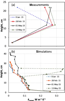
4.3 Measurements vs. simulations of snow ksnow
Our time series ofksnowallow us to test the ability of a de-tailed snow physics model to predict the value of this vari-able. This test is important, as the water vapour flux is an important process in the shaping of Arctic snowpacks. Given that detailed snow physics models such as Crocus (Vionnet et al., 2012) or SNOWPACK (Fierz and Lehning, 2001) do not take into account these fluxes, their ability to predictksnow
needs testing. A paper on SNOWPACK (Bartelt and Lehning, 2002) states that the model does include water vapour fluxes, but the scheme described was never actually implemented in the model (C. Fierz, private communication, 2015). Fig-ure 13 compares our measFig-urements ofksnowwith those
sim-ulated by Crocus. The Crocus runs performed are those de-tailed in Domine et al. (2016) for herb tundra conditions.
It is clear that simulations and measurements yield very different results. Measurements show low values for the lower depth hoar layers and high values for the upper wind slabs. On the contrary, simulations show a value around 0.26 W m−1K−1 for the very basal layer,
indicat-ing a melt–freeze crust, values around 0.12 W m−1K−1 for
the lower depth hoar layers and values always lower than 0.07 W m−1K−1for the upper layers. On 13 May, high
sim-ulated values appear around 22 cm.
Cro-Figure 13. Vertical profiles ofksnow:(a)measured by the needle probes;(b)modelled by CROCUS.
cus simulated a melting episode in late September, giving the basal layer a high thermal conductivity. This is consistent with our observations of a melt–freeze relic in the basal depth hoar layer. However, Crocus cannot predict the transforma-tion of a melt–freeze layer into depth hoar because it does not simulate the required vapour fluxes. These fluxes lead to mass loss in the lower layers and mass gain in the upper ones. This is an important process that contributes to the observed inverted density profiles (Fig. 2) (Sturm and Benson, 1997) and hence the inverted thermal conductivity profiles because thermal conductivity is calculated from density only. The dif-ferences highlighted in Fig. 13 are not due to specificities of Crocus. Simulations with SNOWPACK version 3.30 driven by North American Regional Reanalysis (NARR) data (http: //www.esrl.noaa.gov/psd/data/gridded/data.narr.html) for the same dates (not shown) revealed similar inverted density and thermal conductivity profiles (A. Langlois and J.-B. Madore, personal communication, 2016). The other processes that lead to dense upper layers are wind packing and to a smaller extent weight compaction. The Crocus representation of the wind-packing process cannot be evaluated here, as the den-sity increase also has contributions from water vapour depo-sition due to the upward flux and their respective contribu-tions cannot be observed separately. An appropriate descrip-tion of the water vapour flux is required to test the repre-sentation of wind packing here. In any case, it is clear that omitting vapour fluxes in Arctic snowpacks leads to an
in-adequate simulation of the density and thermal conductivity profile of the snowpack.
A detailed evaluation of the ability of Crocus to reproduce the ground thermal regime is in order. However, ground tem-perature also depends on soil properties so that coupling to a land surface scheme is required for full testing. Crocus is currently coupled to the land surface scheme ISBA through the SURFEX interface. Improved snow and soil schemes for ISBA are being tested (Decharme et al., 2016) and the evalu-ation of these new schemes will be the subject of future work. Lastly, the parameterization of Yen (1981) to calcu-late thermal conductivity from density may not be suit-able for Arctic snow. For a density representative of the depth hoar studied, 200 kg m−3(Yen, 1981) predictsksnow=
0.11 W m−1K−1, while we consistently measured values in the range 0.025 to 0.035 W m−1K−1. The more
re-cent parameterization of Calonne et al. (2011) predicts 0.10 W m−1K−1. That of Löwe et al. (2013) predicts
0.12 W m−1K−1. These parameterization are based on a
lim-ited number of values (30 for Calonne et al., 2011) obtained on alpine or temperate snows that were sampled for mea-surement in the laboratory. This means that they could not work (or do so with extreme difficulty) on low-density depth hoar, as this snow often collapses at the slightest contact. Their data sets then exclude one snow type of particular in-terest to us. Using their data to discuss our work is there-fore irrelevant. By contrast, using the parameterization of Sturm et al. (1997) based on over 500 values of Arctic or subarctic snows predictsksnow=0.065 W m−1K−1. That of Domine et al. (2011) based on 106 alpine and Arctic snows predicts 0.088 W m−1K−1. Both latter studies show values
as low as measured here and also indicate that for a given density value, the range ofksnowvalues varies by a factor of 4 to 5, and our measured values are within this range. These correlation-based estimations ofksnowshow that (i) density– thermal conductivity correlations cannot accurately predict ksnow and (ii) using parameterisations based on a data sets
consisting mostly of alpine or temperate snow cannot be used for Arctic snow.
4.4 Seasonal variations ofksoil
Understanding and predicting the seasonal variations ofksoil
Nordic soils. Here, we provide such data for the soil at our location and these will be used in future work to test our abil-ity to simulate the permafrost thermal regime using the ISBA code (Decharme et al., 2016).
A tempting approximation would be to use a bimodal dis-tribution of thermal conductivity values, as we find transition periods of less than 10 days. The transition from thawed to frozenksoil values takes 6 days in 2013 and 8 days in 2014
(remember that measurements are made every 2 days only). The transition from frozen to thawedksoilvalues takes 2 days
in 2015. In 2014, the data are not of sufficient quality to deter-mine the transition duration accurately. However, a bimodal distribution, despite its advantage of being simple to imple-ment in models, can lead to errors in soil temperature greater than 2◦C, as shown by Smerdon and Mendoza (2010) for
peat. Further work is required to test its interest for our more mineral soil.
5 Conclusion
We feel that the following points are important conclusions of this study:
1. Vertical water vapour fluxes induced by the temperature gradients in the soil and the snowpack strongly deter-mine snow conditions, soil dehydration and the water budget of the surface.
2. Water vapour fluxes also determine the snow thermal conductivity profile and the ground thermal regime. The comparison of observed vs. simulated thermal conduc-tivity profile demonstrates that omitting these fluxes leads to a radically different snow thermal conductivity profile.
3. Major snow models (Crocus, SNOWPACK) do not de-scribe water vapour fluxes. The consequences on the water budget, on the ground thermal regime, on the en-ergy budget of the surface and possibly on climate may be quite significant.
4. For both years studied, a layer of soft depth hoar was present at the base of the snowpack, which seems to be favourable conditions for subnivean life. In the sec-ond year, a melt–freeze layer at the very base of the snow pack may have rendered conditions somewhat less favourable for a few weeks, butksnowmonitoring
indi-cates that it transformed rapidly into depth hoar. In May 2015, however, we observed that basal depth hoar was harder than in May 2014. We note with interest that lem-ming populations were also higher in spring 2014 than in spring 2015 (Fauteux et al., 2016).
5. Soil thermal conductivity showed transition periods of just a few days between the thawed and the frozen val-ues. Modelling soil thermal conductivity with a step
function may therefore be tested. A hysteresis process was observed, with the change from thawed to frozen value taking place at low ice content and the change from frozen to thawed values at high ice content. Fur-ther work is needed to determine wheFur-ther these pro-cesses need to be taken into account for adequate sim-ulation of the permafrost thermal regime at our study site.
The Supplement related to this article is available online at doi:10.5194/tc-10-2573-2016-supplement.
Author contributions. Florent Domine designed research. De-nis Sarrazin built and deployed the instruments with assistance from Florent Domine. Mathieu Barrere and Florent Domine performed the field measurements. Florent Domine and Mathieu Barrere anal-ysed the field data. Mathieu Barrere performed the model simula-tions. Florent Domine prepared the manuscript with comments from Mathieu Barrere and Denis Sarrazin.
Acknowledgements. This work was supported by the French Polar Institute (IPEV) through grant 1042 to FD and by NSERC through the discovery grant program. We thank Laurent Arnaud for advice in writing the program to run the needle probes. The Polar Continental Shelf Program (PCSP) efficiently provided logistical support for the research at Bylot Island. We are grateful to Gilles Gauthier and Marie-Christine Cadieux for their decades-long efforts to build and maintain the research base of the Centre d’Etudes Nordiques at Bylot Island. Winter field trips were shared with the group of Dominique Berteaux, who helped make this research much more efficient and fun. Bylot Island is located within Sirmilik National Park, and we thank Parks Canada and the Pond Inlet community (Mittimatalik) for permission to work there. The assistance of Matthieu Lafaysse, Samuel Morin and Vincent Vionnet at Centre d’Etudes de la Neige (Météo France-CNRS) for the use of Crocus is gratefully acknowledged. We thank J.-B. Madore and A. Langlois (University of Sherbrooke) for sharing with us their results on SNOWPACK simulations. Constructive comments by Martin Schneebeli, Matthew Sturm, an anonymous reviewer, and the editor Ross Brown are gratefully acknowledged.
Edited by: R. Brown
Reviewed by: M. Sturm, M. Schneebeli and one anonymous referee
References
Bartelt, P. and Lehning, M.: A physical SNOWPACK model for the Swiss avalanche warning Part I: numerical model, Cold Reg. Sci. Technol., 35, 123–145, 2002.
Bilodeau, F., Gauthier, G., and Berteaux, D.: The effect of snow cover on lemming population cycles in the Canadian High Arctic, Oecologia, 172, 1007–1016, 2013.
Brun, E., Vionnet, V., Boone, A., Decharme, B., Peings, Y., Valette, R., Karbou, F., and Morin, S.: Simulation of northern Eurasian local snow depth, mass and density using a detailed snowpack model and meteorological reanalysis, J. Hydrometeorol., 14, 203–214, 2013.
Burke, E., Dankers, R., Jones, C., and Wiltshire, A.: A retrospective analysis of pan Arctic permafrost using the JULES land surface model, Clim. Dynam., 41, 1025–1038, 2013.
Buteau, S., Fortier, R., Delisle, G., and Allard, M.: Numerical simu-lation of the impacts of climate warming on a permafrost mound, Permafrost Periglac., 15, 41–57, 2004.
Calonne, N., Flin, F., Morin, S., Lesaffre, B., du Roscoat, S. R., and Geindreau, C.: Numerical and experimental investigations of the effective thermal conductivity of snow, Geophys. Res. Lett., 38, L23501, doi:10.1029/2011GL049234, 2011.
Calonne, N., Geindreau, C., and Flin, F.: Macroscopic Modeling for Heat and Water Vapor Transfer in Dry Snow by Homogenization, J. Phys. Chem. B, 118, 13393–13403, 2014.
Chadburn, S. E., Burke, E. J., Essery, R. L. H., Boike, J., Langer, M., Heikenfeld, M., Cox, P. M., and Friedlingstein, P.: Impact of model developments on present and future simulations of permafrost in a global land-surface model, The Cryosphere, 9, 1505–1521, doi:10.5194/tc-9-1505-2015, 2015.
Colbeck, S. C.: Sintering in a dry snow cover, J. Appl. Phys., 84, 4585–4589, 1998.
Decharme, B., Brun, E., Boone, A., Delire, C., Le Moigne, P., and Morin, S.: Impacts of snow and organic soils parameteri-zation on northern Eurasian soil temperature profiles simulated by the ISBA land surface model, The Cryosphere, 10, 853–877, doi:10.5194/tc-10-853-2016, 2016.
Dee, D. P., Uppala, S. M., Simmons, A. J., Berrisford, P., Poli, P., Kobayashi, S., Andrae, U., Balmaseda, M. A., Balsamo, G., Bauer, P., Bechtold, P., Beljaars, A. C. M., van de Berg, L., Bid-lot, J., Bormann, N., Delsol, C., Dragani, R., Fuentes, M., Geer, A. J., Haimberger, L., Healy, S. B., Hersbach, H., Holm, E. V., Isaksen, L., Kallberg, P., Kohler, M., Matricardi, M., McNally, A. P., Monge-Sanz, B. M., Morcrette, J. J., Park, B. K., Peubey, C., de Rosnay, P., Tavolato, C., Thepaut, J. N., and Vitart, F.: The ERA-Interim reanalysis: configuration and performance of the data assimilation system, Q. J. Roy. Meteor. Soc., 137, 553–597, 2011.
Devries, D. A.: A nonstationary method for determining thermal conductivity of soil insitu, Soil Sci., 73, 83–89, 1952.
Domine, F., Cabanes, A., and Legagneux, L.: Structure, micro-physics, and surface area of the Arctic snowpack near Alert during the ALERT 2000 campaign, Atmos. Environ., 36, 2753– 2765, 2002.
Domine, F., Bock, J., Morin, S., and Giraud, G.: Linking the effec-tive thermal conductivity of snow to its shear strength and its den-sity, J. Geophys. Res., 116, F04027, doi:10.1029/2011JF002000, 2011.
Domine, F., Gallet, J.-C., Bock, J., and Morin, S.: Structure, specific surface area and thermal conductivity of the snow-pack around Barrow, Alaska, J. Geophys. Res., 117, D00R14, doi:10.1029/2011JD016647, 2012.
Domine, F., Barrere, M., Sarrazin, D., Morin, S., and Arnaud, L.: Automatic monitoring of the effective thermal conductivity of snow in a low-Arctic shrub tundra, The Cryosphere, 9, 1265– 1276, doi:10.5194/tc-9-1265-2015, 2015.
Domine, F., Barrere, M., and Morin, S.: The growth of shrubs on high Arctic tundra at Bylot Island: impact on snow physical prop-erties and permafrost thermal regime, Biogeosciences Discuss., doi:10.5194/bg-2016-3, in review, 2016.
Domine, F., Morin, S., Brun, E., Lafaysse, M., and Carmag-nola, C. M.: Seasonal evolution of snow permeability un-der equi-temperature and temperature-gradient conditions, The Cryosphere, 7, 1915–1929, doi:10.5194/tc-7-1915-2013, 2013. Domine, F., Taillandier, A.-S., Cabanes, A., Douglas, T. A.,
and Sturm, M.: Three examples where the specific surface area of snow increased over time, The Cryosphere, 3, 31–39, doi:10.5194/tc-3-31-2009, 2009.
Ekici, A., Chadburn, S., Chaudhary, N., Hajdu, L. H., Marmy, A., Peng, S., Boike, J., Burke, E., Friend, A. D., Hauck, C., Krin-ner, G., Langer, M., Miller, P. A., and Beer, C.: Site-level model intercomparison of high latitude and high altitude soil thermal dynamics in tundra and barren landscapes, The Cryosphere, 9, 1343–1361, doi:10.5194/tc-9-1343-2015, 2015.
Elberling, B., Michelsen, A., Schadel, C., Schuur, E. A. G., Chris-tiansen, H. H., Berg, L., Tamstorf, M. P., and Sigsgaard, C.: Long-term CO2production following permafrost thaw, Nature Clim. Change, 3, 890–894, 2013.
Fauteux, D., Gauthier, G., and Berteaux, D.: Seasonal demography of a cyclic lemming population in the Canadian Arctic, J. Anim. Ecol., 84, 1412–1422, 2015.
Fauteux, D., Gauthier, G., and Berteaux, D.: Top-down limitation of lemmings revealed by experimental reduction of predators, Ecol-ogy, in press, doi:10.1002/ecy.1570, 2016.
Fierz, C. and Lehning, M.: Assessment of the micro structure-based snow-cover model SNOWPACK: thermal and mechanical prop-erties, Cold Reg. Sci. Technol., 33, 123–131, 2001.
Fierz, C., Armstrong, R. L., Durand, Y., Etchevers, P., Greene, E., McClung, D. M., Nishimura, K., Satyawali, P. K., and Sokra-tov, S. A.: The International classification for seasonal snow on the ground UNESCO-IHP, ParisIACS Contribution no. 1, 80 pp., 2009.
Fortier, D. and Allard, M.: Frost-cracking conditions, Bylot Island, Eastern Canadian Arctic Archipelago, Permafrost Periglac., 16, 145–161, 2005.
Gallet, J.-C., Domine, F., Zender, C. S., and Picard, G.: Measument of the specific surface area of snow using infrared re-flectance in an integrating sphere at 1310 and 1550 nm, The Cryosphere, 3, 167–182, doi:10.5194/tc-9-1343-2015, 2009. Gouttevin, I., Menegoz, M., Dominé, F., Krinner, G., Koven,
C., Ciais, P., Tarnocai, C., and Boike, J.: How the insulat-ing properties of snow affect soil carbon distribution in the continental pan-Arctic area, J. Geophys. Res., 117, G02020, doi:10.1029/2011JG001916, 2012.
Hall, D. K., Sturm, M., Benson, C. S., Chang, A. T. C., Foster, J. L., Garbeil, H., and Chacho, E.: Passive microwave remote and insitu measurements of Arctic and sub-arctic snow covers in Alaska, Remote Sens. Environ., 38, 161–172, 1991.
Camill, P., Yu, Z., Palmtag, J., and Kuhry, P.: Estimated stocks of circumpolar permafrost carbon with quantified uncertainty ranges and identified data gaps, Biogeosciences, 11, 6573-6593, doi:10.5194/bg-11-6573-2014, 2014.
Inaba, H.: Experimental-study on thermal-properties of frozen soils, Cold Reg. Sci. Technol., 8, 181–187, 1983.
Kausrud, K. L., Mysterud, A., Steen, H., Vik, J. O., Ostbye, E., Cazelles, B., Framstad, E., Eikeset, A. M., Mysterud, I., Solhoy, T., and Stenseth, N. C.: Linking climate change to lemming cy-cles, Nature, 456, 93–U93, 2008.
Kujala, K., Seppala, M., and Holappa, T.: Physical properties of peat and palsa formation, Cold Reg. Sci. Tech., 52, 408–414, 2008. Löwe, H., Riche, F., and Schneebeli, M.: A general treatment
of snow microstructure exemplified by an improved rela-tion for thermal conductivity, The Cryosphere, 7, 1473–1480, doi:10.5194/tc-7-1473-2013, 2013.
Marbouty, D.: An experimental study of temperature-gradient meta-morphism, J. Glaciol., 26, 303–312, 1980.
Marti, J. and Mauersberger, K.: A survey and new measurements of ice vapor-pressure at temperatures between 170 and 250 K, Geophys. Res. Lett., 20, 363–366, 1993.
Morin, S., Domine, F., Arnaud, L., and Picard, G.: In-situ measure-ment of the effective thermal conductivity of snow, Cold Reg. Sci. Technol., 64, 73–80, 2010.
Overduin, P. P., Kane, D. L., and van Loon, W. K. P.: Measuring thermal conductivity in freezing and thawing soil using the soil temperature response to heating, Cold Reg. Sci. Technol., 45, 8– 22, 2006.
Paquin, J. P. and Sushama, L.: On the Arctic near-surface per-mafrost and climate sensitivities to soil and snow model formu-lations in climate models, Clim. Dynam., 44, 203–228, 2015. Penner, E.: Thermal conductivity of frozen soils, Can. J. Earth Sci.,
7, 982–987, 1970.
Penner, E., Johnston, G. H., and Goodrich, L. E.: Thermal-conductivity laboratory studies of some mackenzie highway soils, Can. Geotech. J., 12, 271–288, 1975.
Riche, F. and Schneebeli, M.: Thermal conductivity of snow mea-sured by three independent methods and anisotropy considera-tions, The Cryosphere, 7, 217–227, doi:10.5194/tc-7-217-2013, 2013.
Schneider von Deimling, T., Meinshausen, M., Levermann, A., Hu-ber, V., Frieler, K., Lawrence, D. M., and Brovkin, V.: Estimating the near-surface permafrost-carbon feedback on global warming, Biogeosciences, 9, 649–665, doi:10.5194/bg-9-649-2012, 2012. Schuur, E. A. G., McGuire, A. D., Schadel, C., Grosse, G., Harden, J. W., Hayes, D. J., Hugelius, G., Koven, C. D., Kuhry, P., Lawrence, D. M., Natali, S. M., Olefeldt, D., Romanovsky, V. E., Schaefer, K., Turetsky, M. R., Treat, C. C., and Vonk, J. E.: Cli-mate change and the permafrost carbon feedback, Nature, 520, 171–179, 2015.
Smerdon, B. D. and Mendoza, C. A.: Hysteretic freezing charac-teristics of riparian peatlands in the Western Boreal Forest of Canada, Hydrol. Process., 24, 1027–1038, 2010.
Spaans, E. J. A. and Baker, J. M.: The soil freezing characteristic: Its measurement and similarity to the soil moisture characteristic, Soil Sci. Soc. Am. J., 60, 13–19, 1996.
Sturm, M. and Benson, C.: Scales of spatial heterogeneity for peren-nial and seasonal snow layers, Ann. Glaciol., 38, 253–260, 2004. Sturm, M. and Benson, C. S.: Vapor transport, grain growth and depth-hoar development in the subarctic snow, J. Glaciol., 43, 42–59, 1997.
Sturm, M., Derksen, C., Liston, G., Silis, A., Solie, D., Holm-gren, J., and Huntington, H.: A reconnaissance snow survey across northwest territories and Nunavut, Canada, April 2007, Cold Regions Research and Engineering laboratory, Hanover, N.H.ERDC/CRREL TR 08-3, 1–80, 2008.
Sturm, M., Holmgren, J., Konig, M., and Morris, K.: The thermal conductivity of seasonal snow, J. Glaciol., 43, 26–41, 1997. Sturm, M., Holmgren, J., and Perovich, D. K.: Winter snow cover
on the sea ice of the Arctic Ocean at the Surface Heat Budget of the Arctic Ocean (SHEBA): Temporal evolution and spatial vari-ability, J. Geophys. Res., 107, 8047, doi:10.1029/2000JC000400, 2002.
Sturm, M. and Johnson, J. B.: Natural-convection in the sub-arctic snow cover, J. Geophys. Res.-Earth, 96, 11657–11671, 1991. Sturm, M. and Johnson, J. B.: Thermal-conductivity measurements
of depth hoar, J. Geophys. Res.-Earth, 97, 2129–2139, 1992. Taillandier, A. S., Domine, F., Simpson, W. R., Sturm, M., Douglas,
T. A., and Severin, K.: Evolution of the snow area index of the subarctic snowpack in central Alaska over a whole season. Con-sequences for the air to snow transfer of pollutants, Environ. Sci. Technol., 40, 7521–7527, 2006.
Taillandier, A. S., Domine, F., Simpson, W. R., Sturm, M., and Dou-glas, T. A.: Rate of decrease of the specific surface area of dry snow: Isothermal and temperature gradient conditions, J. Geo-phys. Res., 112, F03003, doi:10.1029/2006JF000514, 2007. Vionnet, V., Brun, E., Morin, S., Boone, A., Faroux, S., Le Moigne,
P., Martin, E., and Willemet, J.-M.: The detailed snowpack scheme Crocus and its implementation in SURFEX v7.2, Geosci. Model Dev., 5, 773–791, doi:10.5194/gmd-5-773-2012, 2012. Vuichard, N. and Papale, D.: Filling the gaps in meteorological
con-tinuous data measured at FLUXNET sites with ERA-Interim re-analysis, Earth Syst. Sci. Data, 7, 157–171, doi:10.5194/essd-7-157-2015, 2015.