www.atmos-chem-phys.net/17/297/2017/ doi:10.5194/acp-17-297-2017
© Author(s) 2017. CC Attribution 3.0 License.
Particle settling and vertical mixing in the Saharan Air Layer as
seen from an integrated model, lidar, and in situ perspective
Josef Gasteiger1,2, Silke Groß3, Daniel Sauer3, Moritz Haarig4, Albert Ansmann4, and Bernadett Weinzierl2 1Meteorologisches Institut, Ludwig-Maximilians-Universität, München, Germany
2Faculty of Physics, University of Vienna, Vienna, Austria
3Institut für Physik der Atmosphäre, Deutsches Zentrum für Luft- und Raumfahrt, Oberpfaffenhofen, Germany 4Leibniz Institute for Tropospheric Research, Leipzig, Germany
Correspondence to:Josef Gasteiger ([email protected])
Received: 6 June 2016 – Published in Atmos. Chem. Phys. Discuss.: 17 June 2016 Revised: 15 November 2016 – Accepted: 11 December 2016 – Published: 5 January 2017
Abstract.Long-range transport of aerosol in the Saharan Air Layer (SAL) across the Atlantic plays an important role for weather, climate, and ocean fertilization. However, processes occurring within the SAL and their effects on aerosol prop-erties are still unclear. In this work we study particle settling and vertical mixing within the SAL based on measured and modeled vertical aerosol profiles in the upper 1 km of the transported SAL. We use ground-based lidar measurements and airborne particle counter measurements over the western Atlantic, collected during the SALTRACE campaign, as well as space-based CALIOP lidar measurements from Africa to the western Atlantic in the summer season. In our model we take account of the optical properties and the Stokes gravita-tional settling of irregularly shaped Saharan dust particles.
We test two hypotheses about the occurrence of verti-cal mixing within the SAL over the Atlantic to explain the aerosol profiles observed by the lidars and the particle counter. Our first hypothesis (H1) assumes that no mixing occurs in the SAL leading to a settling-induced separation of particle sizes. The second hypothesis (H2) assumes that ver-tical mixing occurs in the SAL allowing large super-micron dust particles to stay airborne longer than without mixing.
The uncertainties of the particle linear depolarization ratio (δl) profiles measured by the ground-based lidars are compa-rable to the modeled differences between H1 and H2 and do not allow us to conclude which hypothesis fits better. The SALTRACE in situ data on size-resolved particle number concentrations show a presence of large particles near the SAL top that is inconsistent with H1. The analysis of the CALIOP measurements also reveals that the averageδl
pro-file over the western Atlantic is inconsistent with H1. Fur-thermore, it was found that the averageδlprofile in the upper 1 km of the SAL does not change along its transport path over the Atlantic. These findings give evidence that vertical mixing within the SAL is a common phenomenon with sig-nificant consequences for the evolution of the size distribu-tion of super-micron dust particles during transport over the Atlantic. Further research is needed to precisely characterize the processes that are relevant for this phenomenon.
1 Introduction
signifi-cant effects for radiative properties and deposition of Saharan aerosols (e.g., Otto et al., 2009; Mahowald et al., 2014).
Size distribution measurements performed at Izaña (Ca-nary Islands) and Puerto Rico (Caribbean) by Maring et al. (2003) revealed that Saharan dust particles withr >3.6 µm are preferentially removed during the transport over the Atlantic. Maring et al. (2003) cannot explain their mea-surements by assuming that Stokes gravitational settling is the only process occurring during transport over the At-lantic. They have to reduce the Stokes settling velocity by 0.0033 m s−1to match the measurements, which could be an indication for vertical mixing of air during the transport. The lack of significant vertical changes of particle size distribu-tions found by Reid et al. (2003) in the Caribbean also indi-cates that settling is counteracted by some other processes.
Lidar remote sensing is a powerful tool for localizing and characterizing aerosols, including their size distributions. The particle linear depolarization ratio δl (Sassen, 1991), measured by advanced lidar systems, is a particularly use-ful parameter for characterizing Saharan aerosols. For ex-ample, in a case study, Liu et al. (2008) characterize a dust outbreak that was transported from the Sahara over the At-lantic. They use measurements of the CALIOP lidar (Winker et al., 2009), which is operated onboard the CALIPSO satel-lite and measures δl at a wavelength of 532 nm. Liu et al. (2013) investigate Asian dust and its transport over the Pa-cific using data from the same instrument. The network EAR-LINET (Pappalardo et al., 2014) provides a comprehensive data set on ground-based lidar measurements throughout Eu-rope, which is useful for studying Saharan aerosols trans-ported to Europe (see e.g., Mattis et al., 2002; Papayannis et al., 2008; Wiegner et al., 2011). During field campaigns like PRIDE (Reid et al., 2003), SAMUM (Heintzenberg, 2009; Ansmann et al., 2011), Fennec (Ryder et al., 2013), and SALTRACE (Weinzierl et al., 2016), Saharan aerosol was measured using a wide set of techniques, including lidar, photometer, and airborne in situ instrumentation. The com-bination of different measurement techniques enables one to better constrain the properties of the rather complex Sa-haran aerosol. Polarization-sensitive (near-) backscattering by dusty aerosols is also studied in laboratories (e.g., Sakai et al., 2010; Järvinen et al., 2016).
Yang et al. (2013) investigate Saharan aerosols on their way over the Atlantic based onδldata from CALIOP. They useδlfrom volumes that the CALIPSO operational algorithm classified as dust-laden and averageδlas function of height above sea level, over the summer season 2007. The averaged
δl profiles show an increasing height dependence with in-creasing distance from Africa. Over the western Atlantic they find the largestδl values at altitudes of about 4–5 km and a decrease ofδlwith decreasing altitude. Yang et al. (2013) ex-plain the averaged CALIOPδlprofiles with settling-induced separation of particle shapes using a model that assumes that particles with nearly spherical shape settle faster and have
smallerδlthan particles with stronger deviation from spheri-cal shape.
In our study we investigate the Saharan aerosol transport over the Atlantic by combining advanced modeling efforts with data obtained from ground-based lidar, airborne particle counters, and the CALIOP lidar. We show theoretical pro-files for Saharan aerosols considering gravitational settling as a function of particle size and shape. We differentiate be-tween two hypotheses about the occurrence of vertical mix-ing within the SAL. The lidar-relevant optical properties are simulated based on the particle microphysics explicitly using an optical model. We compare our modeled profiles with the measured data that we evaluate as a function of distance from the SAL top. The ground-based and airborne measurements used in our study were performed during the SALTRACE field campaign (Weinzierl et al., 2016) in the summer of 2013 in the vicinity of Barbados (Caribbean). From CALIOP, we use nighttime profile data covering 15 summer months and the Saharan aerosol transport region from Africa to the Caribbean.
After describing our modeling approach (Sect. 2) we in-vestigate modeled lidar profiles after 5 days of transport without vertical mixing (Sect. 3.1), which is a typical trans-port time of Saharan aerosol to the Caribbean. The sensitivity ofδlprofiles to particle shape (Sect. 3.2) and to the shape de-pendence of the settling velocity (Sect. 3.3) is subsequently investigated. In Sect. 3.4 we model the effect of daytime con-vective vertical mixing occurring in the SAL during trans-port. Subsequently, the modeled profiles are compared in a case study to lidar and in situ profiles measured in Barba-dos during SALTRACE (Sect. 4) to test our two hypothe-ses about vertical mixing in the SAL over the Atlantic. In Sect. 5 we continue testing these hypotheses by using aver-aged CALIOP profiles before we give concluding remarks in Sect. 6.
2 Model description
We also consider the case of a diurnal cycle of the convective vertical mixing activity.
2.1 Stokes settling
The settling velocityv of a particle relative to the ambient air is determined by the balance between gravitational force
Fgand drag forceFdif other forces can be neglected. The gravitation force is given by
Fg= 4 3π rv
3ρg,
(1) with the volume-equivalent radiusrvof the particle, the grav-itational accelerationg=9.81 m s−2, and the particle density
ρthat we assume to be 2.6×10³kg m−3for mineral dust par-ticles (Hess et al., 1998). The drag force of a settling aerosol particle in the size range ofr≈0.5 µm tor≈10 µm (being in the Stokes drag regime) can be approximated by
Fd=6π ηrcv, (2)
with the dynamic viscosity of airη=17 µPa s (approximate value for a temperature of 0◦C and tropospheric pressures) and the cross-section-equivalent radiusrcof the particle. We userc instead ofrvin this equation because the drag force is related more to the cross section of the particle than to its volume.
We note that using rc in Eq. (2) is an approximation be-cause determining the exact Stokes drag force of an irregu-larly shaped particle is a more complex issue; see e.g., Loth (2008). The drag force of a particle larger than r≈10 µm is stronger than calculated with Eq. (2). For example, in the case of spherical particles,Fdis increased by about 5 % for r=20 µm and about 15 % for r=30 µm compared to Stokes law (Hinds, 1999). In addition, because of the flow around the settling particle, coarse nonspherical particles can become horizontally aligned. Using the formula about the probability distributions of orientation angles of prolate spheroids compiled by Ulanowski et al. (2007), we estimate that settling-induced alignment occurs for dust particles with
r >5 µm. In the Stokes regime, for typical dust aspect ratios of 1.6–1.8, Fd of a spheroid in horizontal orientation is on average about 5 % stronger than the averageFdof the same particle in random orientation (Clift et al., 1978). In the fol-lowing, we stick to Eq. (2) for the calculation ofFdbecause these deviations have only a negligible effect on the profiles presented below.
Setting Fg=Fd and using the conversion factor ξvc=
rv/rc(Gasteiger et al., 2011) results in a settling velocity of the particle relative to the ambient air of
v=2gρ 9η ·r
2 c·ξ
3
vc. (3)
ξvc of our six irregular model shapes is 0.955 (shape A), 0.932 (B), 0.911 (C), 0.871 (D), 0.925 (E), and 0.866 (F).
0 2 4 6 8 10 12
Maximum cross-section-equivalent radius rmax [µm] 0
200
400
600
800
1000
dz [m] ξξvcvc = 0.85 = 0.90
ξvc = 0.95 ξvc = 1.00
ts
= 8 h
ts
= 1 d
ts
= 5 d
Figure 1.Maximum cross-section-equivalent radiusrmaxof dust
particles as a function of distance dzfrom the SAL top after dif-ferent settling time periodstsassuming different shape-dependent
conversion factorsξvc.ξvc=1 corresponds to spherical particles.
Note that the dynamic shape factor χ (Hinds, 1999) is
χ=ξvc−1 ifrvis assumed andχ=ξvc−3if rc is assumed for the radius. Henceforth, unless otherwise stated, we use the cross-section-equivalent radiusr=rcfor describing particle size.
As a result of gravitational settling during a time periodts without vertical mixing, the maximum particle radiusrmaxat a distance dzfrom the upper boundary of the SAL is given by
rmax= s
9ηdz
2gρξ3 vcts
. (4)
Figure 1 illustratesrmaxas function of dzfor different set-tling time periodsts. The solid lines showrmaxfor a conver-sion factorξvc=0.9, which is in the range of our dust model shapes. The vertical axis was chosen such that the top of the SAL (dz=0 m) is at the top of the figure. For example, at
ts=5 d, no particles with radiir >2 µm andξvc=0.9 exist in the upper 400 m of the SAL.
2.2 Hypotheses about occurrence of vertical mixing
Hypothesis H1
Hypothesis H2
Convection Particle settling, no vertical mixing ts
SAL reaches Atlantic
Settling,
no mixing
Sunset Sunrise ts
inight=1
Convection
etc.
Settling,
no mixing
Sunset Sunrise ts
inight=2
Convection Settling,
no mixing
Sunset Sunrise ts
inight=3
Convection
West Africa East Atlantic Towards the Caribbean
Figure 2.Schematic view of timing in hypotheses about the
occur-rence of settling and convective vertical mixing within the SAL.
and Prospero (1972) or further down in Fig. 8). We empha-size that the convection activity studied here is not connected to the convection occurring in the marine boundary layer (which sometimes affects the lower parts of the SAL).
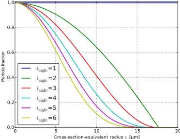
Both hypotheses are illustrated in Fig. 2. We model the transport for one vertical column, ignoring possible wind shear or convergence. For simplicity, we assume that the SAL reaches the Atlantic at first sunset. Furthermore, we assume convective vertical mixing to always be perfect, though in reality convection may be weak and the vertical mixing im-perfect. In the case of H2, the initial aerosol size distribution atts=0 varies from night to night because a certain fraction of particles is removed by settling during the convection-free time each night before convective vertical mixing starts again with sunrise. The fractionf of particles that remains in the SAL after one night is calculated for zsettled(r, ξvc) < HSAL using
f (r, ξvc)=
expHSAL−zsettled(r,ξvc)
Hscale
−1 expHSAL
Hscale
−1
, (5)
wherezsettled(r, ξvc)is the distance the particles have settled during the night. No particles withzsettled(r, ξvc) > HSALare in the SAL after the first night.zsettledis calculated usingv from Eq. (3) and a night duration of 11 h, which is a typical value for the northern tropical Atlantic during summertime.
HSALis the depth of the SAL within which convective verti-cal mixing occurs each day. We useHSAL=3 km. In Eq. (5) we assume that the particles are well-mixed within the SAL at sunset. Those particles that settle during the night below the lower boundary of the SAL (determined by HSAL) are considered as removed from the SAL at sunrise when mixing starts again. Equation (5) considers the exponential decrease of the air density and thus the amount of aerosol (in the case of well-mixed layers) with height. We assume a scale height
Hscale=10 km, which implies an exponential decrease by a factor of efrom the ground to 10 km height. This value of
0 5 10 15 20
Cross-section-equivalent radius rc [µm]
0.0 0.2 0.4 0.6 0.8 1.0
Particle fraction
inight
=1
inight
=2
inight
=3
inight
=4
inight
=5
inight
=6
Figure 3.Fraction of particles (relative to initial size distribution)
existing in SAL at the beginning of each night (ts=0) in the case
of H2 andξvc=0.90.
Hscale was estimated from the tropical standard atmosphere provided by Anderson et al. (1986).
Figure 3 shows the fraction of the particles present in the SAL at the beginning of each night for H2 (counted by
inightas illustrated in Fig. 2). This fraction is calculated from Eq. (5) using
f (r, ξvc)(inight−1) (6)
and is multiplied with the initial aerosol size distribution, which is described below, to get the size distribution at the beginning of each night.
Henceforward in this paper, we denote the hypotheses and points of time using the following notation: for the first hy-pothesis we write [H1,ts] and for the second hypothesis we write [H2,inight,ts].
2.3 Aerosol mixtures and optical modeling
ranges (r <0.1–0.25 µm) consist mainly of ammonium sul-fate. Volatile ammonium sulfate particles were also identified in airborne in situ measurements during SAMUM (Weinzierl et al., 2009) and SALTRACE (Weinzierl et al., 2016).
The mineral dust particles of the reference ensemble are an equiprobable mix of shapes B, C, D, and F (Gasteiger et al., 2011). The optical properties of dust particles with 2π rv/ λ≤25 were calculated with the discrete dipole ap-proximation code ADDA (Yurkin and Hoekstra, 2011) and for larger particles it was assumed that the lidar ratioSand the linear depolarization ratioδlare size-independent, i.e.,S and δl calculated for 2π rv/ λ=25 were also applied for larger particles.
It has been shown for Saharan aerosols that the refractive index varies from dust particle to dust particle (e.g., Kan-dler et al., 2011), and that this variability can have signif-icant effects on lidar-relevant optical properties (Gasteiger et al., 2011). In our model, we consider the refractive index variability using the following approximating approach: the imaginary part of the dust refractive index, which is relevant for absorption, is distributed such that 50 % of the dust par-ticles are non-absorbing while the other 50 % have an imag-inary part that is doubled compared to the value provided by OPAC, leading to good agreement with SAMUM lidar mea-surements (Gasteiger et al., 2011).
We apply a maximum cutoff radiusrmaxthat is varied as a function of distance dzfrom the SAL top as given by Eq. (4). The maximumrmaxis 40 µm (at dz≤1 km only relevant for
ts<1 h). In the case of a diurnal cycle of convective vertical mixing (H2), we additionally consider the partial removal of particles due to settling each night, as described above (Eq. 6, Fig. 3). The evolution of the mineral dust size distribution for H2 (each night atts=0) is illustrated in the Supplement S1. We simulate vertical profiles of the extinction coefficient
α, the backscatter coefficientβ, the lidar ratio
S=α
β =
4π ω0F11(180◦)
, (7)
and the linear depolarization ratio
δl=
1−F22(180◦) / F11(180◦) 1+F22(180◦) / F11(180◦)
. (8)
Here,ω0is the single scattering albedo of the aerosol parti-cles andF11(180◦)andF22(180◦)are elements of their scat-tering matrix at backward direction. We consider the height dependence of the particle concentration of the initially well-mixed layer by multiplying all modeledαandβprofiles with exp(dz / Hscale). In this paper, α, β, S, and δl are always aerosol particle properties, i.e., without gas contributions.
3 Modeled lidar profiles
In this section we first present modeling results for our first hypothesis (H1) with a settling duration of 5 days, which is
the typical time span for transport of aerosol in the SAL from the African coast to Barbados (e.g., Schütz, 1980). H1 is se-lected here because the effects are stronger than in the case of H2. We investigate the sensitivity of theδlprofile to the par-ticle shape and the shape dependence of the settling velocity
v. Finally in the last part of this section, we investigate the effect of the diurnal convective vertical mixing cycle (H2) on theδlprofile.
3.1 Effect of particle settling (H1)
Vertical profiles of lidar-relevant optical properties of the aerosol in the upper 1 km of the SAL, modeled according to H1 after 5 days without vertical mixing of air ([H1, 5 d]) are shown in Fig. 4. The solid lines show results for the refer-ence ensemble at three different lidar wavelengths (indicated by color). To illustrate the effect of the WASO particles, we also consider a case in which we removed all WASO particles (dashed lines of same colors).
The lidar ratio S increases towards the top of the SAL (Fig. 4a).Satλ=532 and 1064 nm has peaks of about 75– 80 sr in the upper 70 m of the SAL, decreasing again in the last few meters below the SAL top. Removing the WASO particles from the ensemble has a significant effect onSonly near the top of the SAL (compare dashed with solid line).
We find a decrease of the linear depolarization ratio δl with decreasing distance dzfrom the SAL top (Fig. 4b). The absolute decrease of δl depends on wavelength; for exam-ple, from dz=1000 m to dz=100 mδldecreases by 0.065, 0.074, and 0.121 at λ=355, 532, and 1064 nm, respec-tively. Removing WASO particles strongly increases δl at all heights, in particular at short wavelengths (compare blue lines forλ=355 nm), illustrating their importance in model-ingδl of Saharan aerosols. The decrease ofδl is shifted to-wards smaller dzif WASO is neglected but the general shape of theδlprofiles does not change.
The backscatter coefficient β, normalized by β at
λ=355 nm and dz=1000 m, is shown in Fig. 4c. It de-creases with decreasing dz, e.g., at dz=100 m and the three lidar wavelengths.β of the reference ensemble is re-duced by 41, 49, and 63 %, respectively, compared toβ at dz=1000 m.
The extinction coefficientα (Fig. 4d) also decreases to-wards the SAL top; the relative decrease, however, is smaller than forβ, e.g., for the reference ensemble we find values of 36, 40, and 50 % for the height levels mentioned above. WASO particles influence the wavelength dependence ofβ
andαat any dz.
40 50 60 70 80 90
Lidar ratioS [sr]
0 200 400 600 800 1000
dz [m]
(a)
0.00 0.05 0.10 0.15 0.20 0.25 0.30 0.35 0.40
Linear depolarization ratioδl
0 200 400 600 800 1000
dz [m]
(b)
Ref. ens. - λ = 355 nm
No WASO - λ = 355 nm
Ref. ens. - λ = 532 nm
No WASO - λ = 532 nm
Ref. ens. - λ = 1064 nm
No WASO - λ = 1064 nm
0.0 0.2 0.4 0.6 0.8 1.0 1.2
Norm alized backscatter coefficient β
0 200 400 600 800 1000
dz [m]
(c)
0.0 0.2 0.4 0.6 0.8 1.0 1.2
Norm alized extinction coefficient α
0 200 400 600 800 1000
dz [m]
(d)
Figure 4.Optical aerosol properties of the upper 1 km of the SAL for [H1, 5 d] assuming the reference ensemble (solid lines) at three lidar
wavelengths (indicated by color).βandαare normalized to the value of the reference ensemble atλ=355 nm and dz=1000 m. The dashed lines present profiles when WASO particles are removed from the reference ensemble.
Figure 5.Linear depolarization ratio profiles atλ=532 nm in the
upper 1 km of the SAL for [H1, 5 d]. The reference ensemble is ap-plied (as in Fig. 4), but only a single dust particle shape is assumed in each profile as indicated in the legend. The approximate aspect ratio is written on each particle.
3.2 Sensitivity ofδlprofiles to particle shape
The shape mixture in our reference ensemble may not be fully representative for desert aerosol. Therefore, it is worth-while to estimate the sensitivity of the lidar profiles to parti-cle shape. Figure 5 showsδl profiles atλ=532 nm for [H1,
5 d] where all dust particles of the reference ensemble were replaced by particles of only a single shape, as indicated in the legend together with their approximate aspect ratios. The other microphysical properties of the dust particles and the properties of the spherical WASO particles were left un-changed. For each profile, the shape-specific ξvc, as given above, is considered in the calculations.
The absolute value ofδl atλ=532 nm depends on par-ticle shape, with a variation range from about 0.2 to 0.4 at dz=1000 m.δlof elongated shapes (C, F) tends to be smaller thanδlof the more compact counterparts (A, E), illustrating that there is no direct correlation between large aspect ratios and largeδl(in contrast to what is often assumed in the lit-erature, e.g., Yang et al., 2013).δldecreases with decreasing dzfor all considered shapes and the decrease is not strongly sensitive to the selection of the particle shape. However, the decrease ofδlin the case of shapes D–F (aggregate particles, edged particles) tends to be shifted to larger dzcompared to
δlin the case of shapes A–C (deformed spheroids). The sensi-tivity ofδlprofiles to realistic changes of the refractive index and the size distribution was found to be lower (not shown) than the sensitivity to the particle shape (Fig. 5).
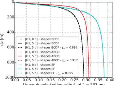
3.3 Sensitivity ofδlprofiles to shape dependence of settling velocity
0.00 0.05 0.10 0.15 0.20 0.25 0.30 0.35 0.40
Linear depolarization ratio δl
at
λ= 532 nm
0
200
400
600
800
1000
dz [m]
[H1, 0 d] - shapes BCDF[H1, 5 d] - shapes BCDF[H1, 5 d] - shapes BCDF - ξvc = 0.895
[H1, 0 d] - shapes ABCD [H1, 5 d] - shapes ABCD
[H1, 5 d] - shapes ABCD - ξvc = 0.917
[H1, 0 d] - shapes EF [H1, 5 d] - shapes EF
[H1, 5 d] - shapes EF - ξvc = 0.895
Figure 6.Analogous to Fig. 5, but assuming mixtures of different
shapes of mineral dust particles as indicated in the legend (shapes BCDF=reference ensemble). The solid lines show profiles for [H1, 5 d]. The dashed lines show the same profiles when no shape depen-dence of the settling velocity is assumed (ξvcof all shapes is set to
the average value, which is given in the legend). The dotted lines show the modeled profile at the beginning of the settling.
settling velocityvbut not the size dependence ofv. Here, we investigate how sensitive δl profiles are to the shape depen-dence ofv compared to the size dependence of v. For this purpose, Fig. 6 showsδlprofiles atλ=532 nm for [H1, 5 d] and for three different shape mixtures, which are indicated by color (mixture BCDF corresponds to the reference ensem-ble used in most other parts of this paper). The solid lines illustrate results when shape-dependent ξvc are considered. By contrast, results shown as dashed lines assumed the av-erage ξvc value (as displayed in the legend) for the settling of all dust shapes, implying that the shape dependence of
v is switched off. For comparison, the initial δl profiles at [H1, 0 d] are also shown as dotted lines. Thus, the differ-ences between the dotted and the solid lines show the total settling effect after 5 days without vertical mixing and the differences between solid and dashed lines show the effect of the shape dependence of the settling velocity. The latter ef-fect is much smaller than the total settling efef-fect, independent of the assumed shape mixture. This allows us to conclude that the settling-induced separation of particle shapes is only of minor importance forδlcompared to the settling-induced separation of particle sizes. These results are consistent with results presented by Ginoux (2003).
3.4 Effect of diurnal convection cycle (H2)
Figure 7 showsδlprofiles for both hypotheses, different time periods without mixing (ts), and different number of nights (inight), assuming our reference ensemble as the initial en-semble. The effect of settling on theδlprofile increases with
0.20
0.22
0.24
0.26
0.28
0.30
Linear depolarization ratio δl
at
λ= 532 nm
0
200
400
600
800
1000
dz [m]
(b)
[H1, 0 d]
[H1, 1 d]
[H1, 3 d]
[H1, 5 d]
[H2, 1, 8 h]
[H2, 2, 8 h]
[H2, 4, 8 h]
[H2, 6, 8 h]
Figure 7.Linear depolarization ratioδlprofiles atλ=532 nm in the
upper 1 km of the SAL for both hypotheses after different transport time periods.
increasingts, in particular in the upper few hundred meters of the SAL (H1, compare dashed lines). In case daytime vertical mixing occurs (H2), the nighttimeδlprofile (shown here for 8 h after sunset) changes only slightly from day to day, with the maximum changes occurring at lower altitudes (compare solid lines). For example, δl is reduced by about 0.007 at dz=1000 m from the first night (inight=1) to the sixth night (inight=6). The differences between the δl profiles for H1 and those for H2 increase with time (lines of same color cor-respond to approximately the same transport time), illustrat-ing the sensitivity of theδlprofiles to the occurrence of ver-tical mixing.
4 Comparison with SALTRACE data
We now discuss our modeling results based on a compari-son with aerosol data measured during the SALTRACE field campaign (Weinzierl et al., 2016) in the upper 1 km of the SAL and test our two hypotheses using this data set. 4.1 Lidar measurements
30 35 40 45 50 Potential temperature [°C] 3800
4000 4200 4400 4600 4800
Height above ground [m]
(a)
Potential temp. Water vapour
0.0 0.5 1.0 1.5 2.0 Bsc. coef. β [10−6· (m sr) ]−1
(b)
β from POLIS [H1, 5 d] [H2, 6, 2 h] POLIS 0:00-0:57UTC
0.0 0.1 0.2 0.3
Linear depol.ratioδl
(c)
δl from POLIS [H1, 5 d] [H2, 6, 2 h] POLIS 0:00-0:57UTC
0.0 0.5 1.0 1.5 2.0 Bsc. coef. β [10−6· (m sr) ]−1
(d)
β from BERTHA [H1, 5 d] [H2, 6, 2 h] BERTHA 23:15-0:45UTC
0.0 0.1 0.2 0.3
Linear depol. ratio δl
(e)
δl from BERTHA [H1, 5 d] [H2, 6, 2 h] BERTHA 23:15-0:45UTC
0 2 4 6 8 10
Water vapour mixing ratio [g kg ]-1
Figure 8.Vertical profiles over Barbados around 00:00 UTC on 11 July 2013.(a)Profile of potential temperature (black) and water vapor
mixing ratio (blue) from a radiosonde launched at 23:39 UTC on 10 July 2013.(b)Particle backscatter coefficientβand(c)particle linear de-polarization ratioδlatλ=532 nm from POLIS measured between 00:00 and 00:57 UTC on 11 July 2013.(d)Particle backscatter coefficient
βand(e)particle linear depolarization ratioδlatλ=532 nm from BERTHA measured between 23:15 UTC on 10 July 2013 and 00:45 UTC
on 11 July 2013. The shaded areas indicate the sum of the systematical and statistical uncertainties of the measured profiles. Corresponding modeled lidar profiles for H1 (red) and H2 (green) are shown. The SAL top heights of the modeled profiles were fitted to the measuredβ
profiles (heights given in main text). A flat smoothing window of about 50 m is used for the measured and modeled lidar profiles.
S and extinction coefficientα. A vertical smoothing length of at least 500 m is required for those properties, but even with this smoothing length the signal-to-noise ratio of the Raman measurements is still too low for a meaningful com-parison with our modeled vertical profiles. Therefore, we restrict our comparison to the linear depolarization ratio δl and the backscatter coefficient β, for which a significantly shorter smoothing length is sufficient. Furthermore, we con-sider onlyλ=532 nm for our comparison.
The lidar measurements presented in this section were per-formed around 00:00 UTC at night from 10 to 11 July 2013. Sunset was at 22:28 UTC. Back trajectory analysis for this air mass using HYSPLIT (Stein et al., 2015) suggests that it had left the African continent about 5 days before the measure-ments (see the Supplement S2). To test our hypotheses about the occurrence of vertical mixing, we assume for this com-parisonts=5 d in the case of H1, andts=2 h andinight=6 in the case of H2.
Figure 8a shows radiosonde data of water vapor mixing ratio (blue) and potential temperature (black). The potential temperature is nearly constant within the SAL, which ex-tends up to about 4600 m above ground. This potential tem-perature profile indicates that vertical mixing might have oc-curred during the transport of this air mass over the Atlantic. The relative humidity at 4500–4600 m is about 50 to 54 %. The vertical structure of the water vapor mixing ratio and the potential temperature might be regarded as typical for the SAL (Carlson and Prospero, 1972).
Figure 8b and c showβandδlprofiles measured by POLIS (black line), temporally averaged over almost 1 h, including the sum of the systematic and statistical uncertainties. Fig-ure 8d and e showβ andδlprofiles measured by BERTHA (black line), temporally averaged over 1.5 h, including the es-timated uncertainties. For comparison, profiles modeled for our hypotheses H1 (red) and H2 (green) are also plotted in Fig. 8. The SAL top heights of the modeled profiles were fitted to the measuredβ profiles. The fitted SAL top height is 4700 m for H1 and 4650 m for H2 in the case of POLIS, whereas it is 4770 m for H1 and 4720 m for H2 in the case of BERTHA. Measured and modeled lidar profiles shown in Fig. 8 were vertically smoothed with a flat window of about 50 m length.
0.000 0.001 0.002 0.003 0.004 0.005 0.006
Ratio of counts of large to small particles
0
200
400
600
800
1000
dz [m]
(a)
count(r=2.5µm) count(r=0.32−0.59µm)
count(r=3.25µm) count(r=0.32−0.59µm)
0.000 0.001 0.002 0.003 0.004 0.005 0.006
Ratio of counts of large to small particles
0
200
400
600
800
1000
dz [m]
(b)
count(r=2.5µm) count(r=0.32−0.59µm)
count(r=3.25µm) count(r=0.32−0.59µm)
0.000 0.001 0.002 0.003 0.004 0.005 0.006
Ratio of counts of large to small particles
0
200
400
600
800
1000
dz [m]
(c)
count(r=2.5µm) count(r=0.32−0.59µm)
count(r=3.25µm) count(r=0.32−0.59µm)
Figure 9.Ratios between counts in different size ranges measured by CAS-DPOL during aircraft ascent and descent(a)between 18:09 and
20:10 UTC on 22 June 2013,(b)between 15:14 and 16:42 UTC on 10 July 2013, and(c)between 12:45 and 13:50 UTC on 11 July 2013. The aircraft locations are illustrated in the Supplement S3. The vertical axis shows the distance from the SAL top. The data were grouped in 100 m wide vertical bins. The error bars are Poisson 95 % confidence intervals.
4.2 Optical particle counter measurements
During SALTRACE, the Cloud and Aerosol Spectrometer with Depolarization Detection (CAS-DPOL manufactured by DMT, Boulder, CO, USA) was operated under a wing of the research aircraft Falcon of the Deutsches Zentrum für Luft- und Raumfahrt (DLR). The ambient air streams through this optical particle counter. It uses a laser as a light source operating atλ=658 nm and measures the intensity of light scattered forward into 4–12◦by individual particles fly-ing through its samplfly-ing area. Each particle is counted and from the measured intensity its size is inverted. The counts are collected in 30 size bins, covering a nominal radius range from 0.25 to 25 µm. These size bins and the size calibration used here were provided by the manufacturer of the instru-ment. The size-resolved in situ data from CAS-DPOL allow us to more directly test the maximum cutoff radius calculated in the case of H1.
For this test we use data from flights performed during daytime on the 22 June and 10 and 11 July 2013. The aircraft
position at the time when the data used here were measured is illustrated in the Supplement S3. To extract the informa-tion about settling-induced separainforma-tion of sizes, we use size bins for which we would expect no counts at low dzdue to settling in the case of H1 and normalize them by counts mea-sured with the same instrument in a size range that is almost not affected by settling (Fig. 1). The results are illustrated in Fig. 9. The blue lines show the counts in the nominal size bin
r=2.5 µm (size bin no. 17), whereas the green lines show the counts in the nominal size binr=3.25 µm (size bin no. 18), both normalized by the counts in the size bins fromr=0.32 to 0.59 µm (size bin nos. 2–9). Analysis of calibration mea-surements performed during SALTRACE suggests that the sizes presented here are underestimated because the instru-ment optics were polluted by dust particles, which reduced the amount of light reaching the detector.
data in 100 m wide vertical bins. The vertical bins are de-scribed by their distance dzfrom the SAL top as determined from the CAS-DPOL data. The SAL top was at 3700 m a.s.l. both during ascent and descent on 22 June, at 5050 m a.s.l. during ascent and at 4900 m a.s.l. during descent on 10 July, and at 4630 m a.s.l. during ascent and at 4550 m a.s.l. during descent on 11 July 2013. Each dzbin covers about 25 s of data, except bins in which the ascent or descent was paused flying at constant altitude.
As illustrated in Fig. 1, in the case of our first hypothe-sis (H1), particles with r≈2.5 µm and larger are removed from dz <550 m after 5 days over the Atlantic. However, the curves in Fig. 9 show that such particles are also detected in the upper 100 m of the SAL near Barbados. This indicates H1 to be unrealistic even if intrinsic uncertainties of the size determination by CAS-DPOL on the order of±50 % are as-sumed. A similar height dependence was also found during the PRIDE campaign, which was based in Puerto Rico (Reid et al., 2003). This suggests that some processes within the SAL keep large particles in the air longer than expected from gravitational settling.
5 Comparison with averageδlprofiles from CALIOP
After presenting SALTRACE case studies in the previous section, we now use averaged CALIOP δl profiles to get a more general view on the modification of the aerosols during the transport over the Atlantic and to test our hypotheses. We note that in reality the SAL transport is much more complex than our hypotheses assume and it varies from case to case. Nonetheless, we expect that averaged profiles of the intensive propertyδl contains evidence about whether the occurrence of vertical mixing within the SAL is typical or not. In the following, we first describe how we calculate the averageδl from the CALIOP data, then compare our modeling results to the averaged profiles in the upper 1 km of the SAL, and finally discuss our findings.
5.1 Averaging CALIOP data
We restrict our analysis to δl at 532 nm because this pa-rameter is relatively insensitive to errors encountered in the extinction-backscatter retrieval (Liu et al., 2013), which may result from uncertainties in the lidar ratio, for example (Wandinger et al., 2010; Amiridis et al., 2013). We again an-alyze the upper 1 km of the SAL, where potential settling and mixing effects should be observable with lidar (Fig. 7). We use CALIPSO level 2 aerosol profile products v3.01 (NASA, 2010) of backscatter coefficients β and the perpendicular components of the backscatter coefficientsβ⊥atλ=532 nm measured during summer 2007–2011, i.e., from June to Au-gust of each of the 5 years. We excluded profiles measured on 23 June and on 2 August 2009 because of unrealistic out-liers found in the data from these days. Powell et al. (2009)
describe how backscattering quantities are calculated from the CALIOP raw data. Vaughan et al. (2009) show the auto-mated procedure for detecting aerosol and cloud layers using these backscattering quantities, and Liu et al. (2009) demon-strate how aerosols are discriminated from clouds. We re-strict our evaluation to measurements in the region from 10 to 30◦N and 0 to 75◦W. We group these measurements in three longitude ranges of 25◦width along the transport path from Africa to the western Atlantic. Only nighttime measure-ments are considered; all measuremeasure-ments were performed ap-proximately 8 h after sunset.
The CALIOP measurements are performed with a verti-cal resolution of 30 m and a horizontal resolution of 330 m. The backscatter coefficientsβ and β⊥ are provided in the level 2 data with a vertical resolution of 60 m (i.e., for bins of 60 m height) and a horizontal resolution of 5 km, which reduces the noise compared to the measured resolution. As discussed by Vaughan et al. (2009), aerosol features are de-tected with 30 m vertical resolution using an iterative pro-cedure starting with the horizontal resolution of 5 km. Since the noise can be considerable at 5 km resolution, in particular if particle concentrations are low, the horizontal resolution is subsequently increased to 20 and 80 km to also detect weaker features. Depending on the results of the feature detection, the backscatter coefficients are horizontally averaged over 5, 20, or 80 km, and the horizontal averaging range can depend on height. In the following we use only data horizontally av-eraged over 5 km.
From the large set of aerosol profiles, profiles that fulfill the following criteria are selected for averaging:
– The uppermost aerosol-containing bin is between 3 and 8 km a.s.l.
– Both sub-bins (30 m height each) of the upper-most containing bin are classified as aerosol-containing.
– All 16 bins (i.e., up to ≈1 km) below the uppermost containing bin are also classified as aerosol-containing.
– No cloud-containing bin is detected in or above the 17 uppermost aerosol-containing bins.
– Data is horizontally averaged over 5 km (not 20 or 80 km) in each of the 17 uppermost aerosol-containing bins.
– Linear depolarization ratioδl, averaged over the 17 up-permost aerosol-containing bins, is larger than 0.10.
βandβ⊥of each of the 17 vertical bins is summed up over all selected profiles. From these sums, the averageδlfor each bin is calculated according to
δl= P
β⊥ P
β−P
β⊥
0.15
0.20
0.25
0.30
Linear depolarization ratio δl
at
λ= 532 nm
0
200
400
600
800
1000
dz [m]
[H1, 0 d][H1, 2 d][H1, 5 d][H2, 1, 8 h] [H2, 3, 8 h] [H2, 6, 8 h] CALIOP 0-25W CALIOP 25-50W CALIOP 50-75W
Figure 10.Linear depolarization ratioδlprofiles atλ=532 nm in
the upper 1 km of the SAL. CALIOP profiles averaged over profiles from summer months 2007 to 2011 that fulfill conditions listed in the text are shown as solid blue, green, and red lines. The colors de-note different longitude ranges. Error bars of the CALIOP profiles show the estimated statistical uncertainty1δlof the averageδl. For
comparison model results for both hypotheses are also shown as dotted (H1) and dashed (H2) lines.
The measurement uncertainties1βand1β⊥provided in the CALIOP profile data are based on a simplified analysis as-suming that all the uncertainties are random, uncorrelated, and produce no biases (Young, 2010). The magnitude of the uncertainties is mainly determined by the signal-to-noise ra-tio (Hunt et al., 2009). To calculate the estimated statistical uncertainty1δl of the averageδlvalue for each bin (Eq. 9), we sum up the squares of the measurement uncertainties of each profile and use
1δl= q
P β2·P
(1β⊥)2+ Pβ⊥ 2
·P (1β)2
P
β−P
β⊥
2 . (10)
As we average over a large number of profiles, the uncertain-ties of the averaged profiles are reduced considerably com-pared to the uncertainties of single profiles.
5.2 Comparison with averaged profiles
Figure 10 shows the averagedδlprofiles calculated from the CALIOP profile data considering all profiles that fulfilled the abovementioned criteria. The averaged data of the uppermost bin are plotted at dz≈30 m, the subsequent bin at dz≈90 m, etc. While the solid blue line shows the averageδl close to the aerosol source region, the distance from the source re-gion increases with the green line (central Atlantic) and red line (western Atlantic). A map illustrating these regions is provided in the Supplement S4. Averages were taken over 9061, 9114, and 3846 individual profiles in the three
respec-tive regions along the SAL transport path. Considering the statistical uncertainty of the average, the averageδldoes not vary along the SAL transport path and is height-independent with values close to 0.30 for dz >250 m.δldecreases towards the SAL top to values of about 0.23–0.25 in the uppermost bin.
Comparing the measured with the modeled profiles, it be-comes clear that the strong decrease ofδlin the upper 100 m of the SAL, as modeled for long-range transport without ver-tical mixing (H1, dotted red line), is not found in the aver-aged CALIOP data over the western Atlantic (solid red line). This indicates that our first hypothesis (H1) is unrealistic. A further result that renders H1 unlikely is the fact that the aver-ageδlprofile from CALIOP is not modified during transport, while one would expect significant changes of theδlprofile during transport if H1 is assumed (compare the dotted lines of different colors).
The dashed lines in Fig. 10 show theδlprofile when day-time convective vertical mixing is assumed (H2). These mod-eledδl profiles are relatively height-independent, except in the upper 100 m of the SAL. Figure 10 shows that consid-ering vertical mixing (using H2 instead of H1) considerably reduces the deviation of the model from the measurements after long-range transport. The measured invariability of the averageδlprofile between the different regions is also much better captured if H2 is assumed. Our model for H2 predicts a reduction ofδlby about 0.007 at dz=1 km after about 5 days (see dashed lines). This reduction is not seen in the CALIOP profiles, possibly because it is within the range of the statis-tical uncertainty of the averagedδlprofiles from CALIOP. 5.3 Discussion of comparison with averaged profiles
Our model assuming daytime vertical mixing (H2) explains the averaged CALIOP data and their invariability between the regions for the most part. However, deviations of theδl profile between this model and the averaged CALIOP data occur in the upper 2–3 bins (compare dashed to solid lines in Fig. 10). The measurements indicate on average a stronger removal of large particles in the upper 100 m of the SAL over Africa and over the Atlantic than H2 suggests. We again emphasize that we average over a large number of different cases. Theδl profiles may vary from case to case, which is hard to quantify from the CALIOP data however because of large statistical uncertainties of single profiles.
con-siderations is that the measuredδlprofile seems to be inde-pendent of region, while one would expect that such effects become larger with distance from the source regions.
Another source of uncertainty is related to our aerosol model. Natural desert aerosol has very complex microphys-ical properties (e.g., Kandler et al., 2011), and as a sequence, our model of the Saharan aerosol mixtures con-tains several assumptions and the calculated optical proper-ties are connected with uncertainproper-ties. Though we argue that our model mixture represents lidar-relevant optical properties of Saharan aerosols well (Gasteiger et al., 2011), we can not exclude that the deviations of the modeled δl profiles (H2) from the averaged measurements in the upper 2–3 bins are related to assumptions in our aerosol mixture and the optical modeling approach.
A further aspect that needs to be kept in mind is that multiple scattering could affect the CALIOP measurements (Wandinger et al., 2010). In the case of our SAL top study, the multiple scattering effect would increase with increasing dzsince the lidar pulse penetrates the SAL from its top. It is well-known that with an increasing amount of particles the multiple scattering effect increases (e.g., Bissonnette et al., 1995). Using the CALIOP profile data, we do not find a sig-nificant dependence of theδl profiles on the absolute values ofβ(not shown), indicating that multiple scattering does not significantly affect the averagedδlprofiles.
To investigate the CALIOP profiles in more detail, an anal-ysis is provided in the Supplement S4, also considering 20 and 80 km horizontal averages, year-by-year variability, sub-bin classification, cloud-aerosol discrimination, and sensitiv-ity to theδlthreshold. The sensitivity of the averagedδl pro-file to these parameters was found to be low. As a conse-quence, it seems likely that the simplifications in H2 (includ-ing the optical model) are the reason for the remain(includ-ing de-viations near the SAL top. The averageβ profile (see Sup-plement S4), as well as the variability of the backscatter co-efficient β from case to case (not shown), can also not be explained using H2, showing the need to consider in future research further aspects for precise SAL transport modeling.
6 Summary and conclusions
Transport of aerosol in the Saharan Air Layer (SAL) over the Atlantic is relevant for weather and climate but important processes within the SAL still are not well understood. To gain insights into relevant processes, we developed a model that describes the modification of the vertical aerosol distri-bution in the upper 1 km of the SAL during transport based on the physical processes of gravitational settling and verti-cal mixing. From the vertiverti-cal aerosol distributions, lidar pro-files are calculated using explicit optical modeling. Sensitiv-ity studies revealed (a) that generally the particle linear de-polarization ratio decreases towards the SAL top for all con-sidered model shapes and (b) that the size dependence of the
settling velocity is significantly more important for the linear depolarization ratio profile than the shape dependence of the settling velocity.
The model results were compared to lidar and in situ mea-surements and two hypotheses about the occurrence of verti-cal mixing within the SAL were tested (H1 without mixing, H2 with mixing during the day). Comparisons with ground-based depolarization lidar measurements in Barbados, per-formed in the framework of the SALTRACE campaign, re-vealed that the measurement uncertainties are in the same order as the differences between both hypotheses. Vertically resolved in situ measurements of the size distribution dur-ing SALTRACE found large particles in the upper part of the SAL that are not consistent with H1, indicating that verti-cal mixing occurs in the SAL over the Atlantic. These find-ings are supported by results from an analysis using night-time data from CALIOP. The CALIOP data show that the average linear depolarization ratio profile in the upper 1 km of the SAL does not change along its transport path over the Atlantic, which disproves H1. These findings are consistent with results from other studies, which found that long-range transported Saharan aerosol contains unexpectedly large par-ticles or that the aerosol properties do not change signifi-cantly during long-range transport, e.g., Reid et al. (2003); Maring et al. (2003); Weinzierl et al. (2011, 2016); Ma-howald et al. (2014); Denjean et al. (2016a, b); van der Does et al. (2016).
We could show that vertical mixing occurs within the SAL, and our model assuming daytime vertical mixing (H2), which is driven by the idea that the Saharan aerosol absorbs sunlight triggering convection, explains most data quite well. However, there are limitations of this idealized model. For example, profiles of extensive properties like the backscatter coefficient can often not be explained with H2, and remain-ing deviations from the averaged CALIOP depolarization data are still unexplained. We did not consider the possibil-ity of weak vertical mixing, or size-selective particle removal at the lower boundary of the SAL during vertical mixing, or effects due to electrical fields in the SAL. Radiative effects in the thermal infrared might be an important aspect for un-derstanding the vertical mixing in the SAL, as discussed by Carlson and Prospero (1972). The development of turbulence due to vertical wind shear, more realistic air layer dynamics, and feedbacks of radiative effects with the dynamics (Chen et al., 2010) are further possible aspects to be considered for a precise understanding of the processes within the SAL, their variability, and their effect on size distributions and lifetime of super-micron particles.
7 Data availability
CALIOP data were obtained via https://eosweb.larc.nasa. gov/project/calipso/cal_lid_l2_05kmapro-prov-v3-01_table.
The Supplement related to this article is available online at doi:10.5194/acp-17-297-2017-supplement.
Acknowledgements. The research leading to these results received
funding from LMU Munich’s Institutional Strategy LMUexcel-lent within the framework of the German Excellence Initiative and from the European Research Council under the European Community’s Horizon 2020 research and innovation framework program, ERC grant agreement no. 640458 – A-LIFE. Silke Groß acknowledges funding by a DLR VO-R young investigator group. The SALTRACE campaign was mainly funded by the Helmholtz Association, DLR, LMU, and TROPOS. The Caribbean Institute for Meteorology and Hydrology in Bridgetown, Barbados, kindly provided the infrastructure to perform the SALTRACE lidar measurements. The CALIOP data were obtained from the NASA Langley Research Center Atmospheric Science Data Center. We are grateful to Volker Freudenthaler for fruitful discussions on our model and the lidar data. We thank the reviewers for their suggestions that helped us to substantially improve our paper.
Edited by: C. Hoose
Reviewed by: two anonymous referees
References
Althausen, D., Müller, D., Ansmann, A., Wandinger, U., Hube, H., Clauder, E., and Zörner, S.: Scanning 6-Wavelength 11-Channel Aerosol Lidar, J. Atmos. Ocean. Technol., 17, 1469–1482, doi:10.1175/1520-0426(2000)017<1469:SWCAL>2.0.CO;2, 2000.
Amiridis, V., Wandinger, U., Marinou, E., Giannakaki, E., Tsekeri, A., Basart, S., Kazadzis, S., Gkikas, A., Taylor, M., Baldasano, J., and Ansmann, A.: Optimizing CALIPSO Saharan dust retrievals, Atmos. Chem. Phys., 13, 12089–12106, doi:10.5194/acp-13-12089-2013, 2013.
Anderson, G. P., Clough, S. A., Kneizys, F. X., Chetwynd, J. H., and Shettle, E. P.: AFGL atmospheric constituent profiles (0– 120 km), Tech. rep., AFGL-TR-86-0110, Environemental Re-search papers No. 954, 1986.
Ansmann, A., Petzold, A., Kandler, K., Tegen, I., Wendisch, M., Müller, D., Weinzierl, B., Müller, T., and Heintzen-berg, J.: Saharan Mineral Dust Experiments SAMUM-1 and SAMUM-2: What have we learned?, Tellus B, 63, 403–429, doi:10.1111/j.1600-0889.2011.00555.x, 2011.
Ben-Ami, Y., Koren, I., and Altaratz, O.: Patterns of North African dust transport over the Atlantic: winter vs. summer, based on CALIPSO first year data, Atmos. Chem. Phys., 9, 7867–7875, doi:10.5194/acp-9-7867-2009, 2009.
Bissonnette, L. R., Bruscaglioni, P., Ismaelli, A., Zaccanti, G., Cohen, A., Benayahu, Y., Kleiman, M., Egert, S., Flesia, C., Schwendimann, P., Starkov, A. V., Noormohammadian, M., Op-pel, U. G., Winker, D. M., Zege, E. P., Katsev, I. L., and Polonsky,
I. N.: LIDAR multiple scattering from clouds, Appl. Phys. B, 60, 355–362, doi:10.1007/BF01082271, 1995.
Carlson, T. N. and Prospero, J. M.: The large-scale move-ment of Saharan air outbreaks over the northern equatorial Atlantic, J. Appl. Meteor., 11, 283–297, doi:10.1175/1520-0450(1972)011<0283:TLSMOS>2.0.CO;2, 1972.
Chen, S.-H., Wang, S.-H., and Waylonis, M.: Modification of Sa-haran air layer and environmental shear over the eastern Atlantic Ocean by dust-radiation effects, J. Geophys. Res.-Atmos., 115, D21202, doi:10.1029/2010JD014158, 2010.
Clift, R., Grace, J. R., and Weber, M. E.: Bubbles, Drops, and Par-ticles, Academic Press, 380 pp., 1978.
Cuesta, J., Marsham, J. H., Parker, D. J., and Flamant, C.: Dynami-cal mechanisms controlling the vertiDynami-cal redistribution of dust and the thermodynamic structure of the West Saharan atmospheric boundary layer during summer, Atmos. Sci. Lett., 10, 34–42, doi:10.1002/asl.207, 2009.
Denjean, C., Cassola, F., Mazzino, A., Triquet, S., Chevaillier, S., Grand, N., Bourrianne, T., Momboisse, G., Sellegri, K., Schwarzenbock, A., Freney, E., Mallet, M., and Formenti, P.: Size distribution and optical properties of mineral dust aerosols transported in the western Mediterranean, Atmos. Chem. Phys., 16, 1081–1104, doi:10.5194/acp-16-1081-2016, 2016a. Denjean, C., Formenti, P., Desboeufs, K., Chevaillier, S.,
Tri-quet, S., Maillé, M., Cazaunau, M., Laurent, B., Mayol-Bracero, O. L., Vallejo, P., Quiñones, M., Gutierrez-Molina, I. E., Cas-sola, F., Prati, P., Andrews, E., and Ogren, J.: Size distribu-tion and optical properties of African mineral dust after inter-continental transport, J. Geophys. Res.-Atmos., 121, 7117–7138, doi:10.1002/2016JD024783, 2016b.
Esselborn, M., Wirth, M., Fix, A., Weinzierl, B., Rasp, K., Tesche, M., and Petzold, A.: Spatial distribution and optical proper-ties of Saharan dust observed by airborne high spectral res-olution lidar during SAMUM 2006, Tellus B, 61, 131–143, doi:10.1111/j.1600-0889.2008.00394.x, 2009.
Freudenthaler, V., Seefeldner, M., Groß, S., and Wandinger, U.: Ac-curacy of linear depolarization ratios in clean air ranges mea-sured with POLIS-6 at 355 and 532 nm, EPJ Web of Conferences, 119, 25013, doi:10.1051/epjconf/201611925013, 2016. Gasteiger, J., Wiegner, M., Groß, S., Freudenthaler, V., Toledano,
C., Tesche, M., and Kandler, K.: Modeling lidar-relevant optical properties of complex mineral dust aerosols, Tellus B, 63, 725– 741, doi:10.1111/j.1600-0889.2011.00559.x, 2011.
Ginoux, P.: Effects of nonsphericity on mineral dust modeling, J. Geophys. Res.-Atmos., 108, 4052, doi:10.1029/2002JD002516, 2003.
Groß, S., Freudenthaler, V., Schepanski, K., Toledano, C., Schäfler, A., Ansmann, A., and Weinzierl, B.: Optical properties of long-range transported Saharan dust over Barbados as measured by dual-wavelength depolarization Raman lidar measurements, Atmos. Chem. Phys., 15, 11067–11080, doi:10.5194/acp-15-11067-2015, 2015.
Heintzenberg, J.: The SAMUM-1 experiment over Southern Morocco: overview and introduction, Tellus B, 61, 2–11, doi:10.1111/j.1600-0889.2008.00403.x, 2009.
Hess, M., Koepke, P., and Schult, I.: Optical Properties of Aerosols and Clouds: The Software Package OPAC, B. Am. Meteor. Soc., 79, 831–844, doi:10.1175/1520-0477(1998)079<0831:OPOAAC>2.0.CO;2, 1998.
Hinds, W. C.: Aerosol technology: properties, behavior, and mea-surement of airborne particles, John Wiley & Sons, 504 pp., 1999.
Hunt, W. H., Winker, D. M., Vaughan, M. A., Powell, K. A., Lucker, P. L., and Weimer, C.: CALIPSO Lidar Description and Perfor-mance Assessment, J. Atmos. Ocean. Technol., 26, 1214–1228, doi:10.1175/2009JTECHA1223.1, 2009.
Järvinen, E., Kemppinen, O., Nousiainen, T., Kociok, T., Möh-ler, O., Leisner, T., and Schnaiter, M.: Laboratory in-vestigations of mineral dust near-backscattering depolariza-tion ratios, J. Quant. Spectrosc. Rad. Trans., 178, 192–208, doi:10.1016/j.jqsrt.2016.02.003, 2016.
Kaaden, N., Massling, A., Schladitz, A., Müller, T., Kandler, K., Schütz, L., Weinzierl, B., Petzold, A., Tesche, M., Lein-ert, S., Deutscher, C., EbLein-ert, M., Weinbruch, S., and Wieden-sohler, A.: State of mixing, shape factor, number size distribu-tion, and hygroscopic growth of the Saharan anthropogenic and mineral dust aerosol at Tinfou, Morocco, Tellus B, 61, 51–63, doi:10.1111/j.1600-0889.2008.00388.x, 2009.
Kandler, K., Lieke, K., Benker, N., Emmel, C., Küpper, M., Müller-Ebert, D., Scheuvens, D., Schladitz, A., Schütz, L., and Wein-bruch, S.: Electron microscopy of particles collected at Praia, Cape Verde, during the Saharan Mineral dust experiment: parti-cle chemistry, shape, mixing state and complex refractive index, Tellus B, 63, 475–496, doi:10.1111/j.1600-0889.2011.00550.x, 2011.
Knippertz, P., Ansmann, A., Althausen, D., Müller, D., Tesche, M., Bierwirth, E., Dinter, T., Müller, T., Von Hoyningen-Huene, W., Schepanski, K., Wendisch, M., Heinold, B., Kandler, K., Pet-zold, A., Schütz, L., and Tegen, I.: Dust mobilization and trans-port in the northern Sahara during SAMUM 2006 – a mete-orological overview, Tellus B, 61, 12–31, doi:10.1111/j.1600-0889.2008.00380.x, 2009.
Koepke, P., Gasteiger, J., and Hess, M.: Technical Note: Optical properties of desert aerosol with non-spherical mineral parti-cles: data incorporated to OPAC, Atmos. Chem. Phys., 15, 5947– 5956, doi:10.5194/acp-15-5947-2015, 2015.
Liu, Z., Omar, A., Vaughan, M., Hair, J., Kittaka, C., Hu, Y., Powell, K., Trepte, C., Winker, D., Hostetler, C., Ferrare, R., and Pierce, R.: CALIPSO lidar observations of the optical properties of Sa-haran dust: A case study of long-range transport, J. Geophys. Res., 113, D07207, doi:10.1029/2007JD008878, 2008.
Liu, Z., Vaughan, M., Winker, D., Kittaka, C., Getzewich, B., Kuehn, R., Omar, A., Powell, K., Trepte, C., and Hostetler, C.: The CALIPSO Lidar Cloud and Aerosol Dis-crimination: Version 2 Algorithm and Initial Assessment of Performance, J. Atmos. Ocean. Technol., 26, 1198–1213, doi:10.1175/2009JTECHA1229.1, 2009.
Liu, Z., Fairlie, T. D., Uno, I., Huang, J., Wu, D., Omar, A., Kar, J., Vaughan, M., Rogers, R., Winker, D., Trepte, C., Hu, Y., Sun, W., Lin, B., and Cheng, A.: Transpacific transport and evolution
of the optical properties of Asian dust, J. Quant. Spectrosc. Rad. Trans., 116, 24–33, doi:10.1016/j.jqsrt.2012.11.011, 2013. Loth, E.: Drag of non-spherical solid particles of
regu-lar and irreguregu-lar shape, Powder Technol., 182, 342–353, doi:10.1016/j.powtec.2007.06.001, 2008.
Mahowald, N., Albani, S., Kok, J. F., Engelstaeder, S., Scanza, R., Ward, D. S., and Flanner, M. G.: The size distribution of desert dust aerosols and its impact on the Earth system, Aeolian Res., 15, 53–71, doi:10.1016/j.aeolia.2013.09.002, 2014.
Maring, H., Savoie, D. L., Izaguirre, M. A., Custals, L., and Reid, J. S.: Mineral dust aerosol size distribution change dur-ing atmospheric transport, J. Geophys. Res.-Atmos., 108, 8592, doi:10.1029/2002JD002536, 2003.
Mattis, I., Ansmann, A., Müller, D., Wandinger, U., and Althausen, D.: Dual-wavelength Raman lidar observations of the extinction-to-backscatter ratio of Saharan dust, Geophys. Res. Lett., 29, 20-1–20-4, doi:10.1029/2002GL014721, 2002.
NASA: CALIPSO Lidar Level 2
Aerosol Profile Products Version 3.01,
doi:10.5067/CALIOP/CALIPSO/CAL_LID_L2_05kmAPro-Prov-V3-01_L2-003.01, 2010.
Otto, S., Bierwirth, E., Weinzierl, B., Kandler, K., Esselborn, M., Tesche, M., Schladitz, A., Wendisch, M., and Trautmann, T.: So-lar radiative effects of a Saharan dust plume observed during SA-MUM assuming spheroidal model particles, Tellus B, 61, 270– 296, doi:10.1111/j.1600-0889.2008.00389.x, 2009.
Papayannis, A., Amiridis, V., Mona, L., Tsaknakis, G., Balis, D., Bösenberg, J., Chaikovski, A., de Tomasi, F., Grigorov, I., Mattis, I., Mitev, V., Müller, D., Nickovic, S., Pérez, C., Pietruczuk, A., Pisani, G., Ravetta, F., Rizi, V., Sicard, M., Trickl, T., Wiegner, M., Gerding, M., Mamouri, R. E., D’Amico, G., and Pappalardo, G.: Systematic lidar observations of Saharan dust over Europe in the frame of EARLINET (2000–2002), J. Geophys. Res., 113, D10204, doi:10.1029/2007JD009028, 2008.
Pappalardo, G., Amodeo, A., Apituley, A., Comeron, A., Freuden-thaler, V., Linné, H., Ansmann, A., Bösenberg, J., D’Amico, G., Mattis, I., Mona, L., Wandinger, U., Amiridis, V., Alados-Arboledas, L., Nicolae, D., and Wiegner, M.: EARLINET: to-wards an advanced sustainable European aerosol lidar network, Atmos. Meas. Tech., 7, 2389–2409, doi:10.5194/amt-7-2389-2014, 2014.
Powell, K. A., Hostetler, C. A., Vaughan, M. A., Lee, K.-P., Trepte, C. R., Rogers, R. R., Winker, D. M., Liu, Z., Kuehn, R. E., Hunt, W. H., and Young, S. A.: CALIPSO Lidar Calibration Algo-rithms. Part I: Nighttime 532-nm Parallel Channel and 532-nm Perpendicular Channel, J. Atmos. Ocean. Technol., 26, 2015– 2033, doi:10.1175/2009JTECHA1242.1, 2009.
Prospero, J. M. and Carlson, T. N.: Vertical and areal distribution of Saharan dust over the western equatorial North Atlantic Ocean, J. Geophys. Res., 77, 5255–5265, doi:10.1029/JC077i027p05255, 1972.
the Puerto Rico Dust Experiment (PRIDE), J. Geophys. Res.-Atmos., 108, 8586, doi:10.1029/2002JD002493, 2003.
Ryder, C. L., Highwood, E. J., Rosenberg, P. D., Trembath, J., Brooke, J. K., Bart, M., Dean, A., Crosier, J., Dorsey, J., Brind-ley, H., Banks, J., Marsham, J. H., McQuaid, J. B., Sodemann, H., and Washington, R.: Optical properties of Saharan dust aerosol and contribution from the coarse mode as measured during the Fennec 2011 aircraft campaign, Atmos. Chem. Phys., 13, 303– 325, doi:10.5194/acp-13-303-2013, 2013.
Sakai, T., Nagai, T., Zaizen, Y., and Mano, Y.: Backscattering lin-ear depolarization ratio measurements of mineral, sea-salt, and ammonium sulfate particles simulated in a laboratory chamber, Appl. Opt., 49, 4441–4449, doi:10.1364/AO.49.004441, 2010. Sassen, K.: The Polarization Lidar Technique for Cloud
Research: A Review and Current Assessment, B. Am. Meteor. Soc., 72, 1848–1866, doi:10.1175/1520-0477(1991)072<1848:TPLTFC>2.0.CO;2, 1991.
Schütz, L.: Long range transport of desert dust with special em-phasis on the Sahara, Ann. NY Acad. Sci., 338, 515–532, doi:10.1111/j.1749-6632.1980.tb17144.x, 1980.
Stein, A. F., Draxler, R. R., Rolph, G. D., Stunder, B. J. B., Cohen, M. D., and Ngan, F.: NOAA’s HYSPLIT Atmospheric Trans-port and Dispersion Modeling System, B. Am. Meteor. Soc., 96, 2059–2077, doi:10.1175/BAMS-D-14-00110.1, 2015.
Tsamalis, C., Chédin, A., Pelon, J., and Capelle, V.: The sea-sonal vertical distribution of the Saharan Air Layer and its mod-ulation by the wind, Atmos. Chem. Phys., 13, 11235–11257, doi:10.5194/acp-13-11235-2013, 2013.
Ulanowski, Z., Bailey, J., Lucas, P. W., Hough, J. H., and Hirst, E.: Alignment of atmospheric mineral dust due to electric field, At-mos. Chem. Phys., 7, 6161–6173, doi:10.5194/acp-7-6161-2007, 2007.
van der Does, M., Korte, L. F., Munday, C. I., Brummer, G.-J. A., and Stuut, G.-J.-B. W.: Particle size traces modern Saharan dust transport and deposition across the equatorial North At-lantic, Atmos. Chem. Phys., 16, 13697–13710, doi:10.5194/acp-16-13697-2016, 2016.
Vaughan, M. A., Powell, K. A., Kuehn, R. E., Young, S. A., Winker, D. M., Hostetler, C. A., Hunt, W. H., Liu, Z., McGill, M. J., and Getzewich, B. J.: Fully Automated De-tection of Cloud and Aerosol Layers in the CALIPSO Li-dar Measurements, J. Atmos. Ocean. Technol., 26, 2034–2050, doi:10.1175/2009JTECHA1228.1, 2009.
Wandinger, U., Tesche, M., Seifert, P., Ansmann, A., Müller, D., and Althausen, D.: Size matters: Influence of multiple scattering on CALIPSO light-extinction profiling in desert dust, Geophys. Res. Lett., 37, L10801, doi:10.1029/2010GL042815, 2010.
Weinzierl, B., Petzold, A., Esselborn, M., Wirth, M., Rasp, K., Kan-dler, K., Schütz, L., Koepke, P., and Fiebig, M.: Airborne mea-surements of dust layer properties, particle size distribution and mixing state of Saharan dust during SAMUM 2006, Tellus B, 61, 96–117, doi:10.1111/j.1600-0889.2008.00392.x, 2009.
Weinzierl, B., Sauer, D., Esselborn, M., Petzold, A., Veira, A., Rose, M., Mund, S., Wirth, M., Ansmann, A., Tesche, M., Groß, S., and Freudenthaler, V.: Microphysical and optical properties of dust and tropical biomass burning aerosol layers in the Cape Verde re-gion - An overview of the airborne in situ and lidar measurements during SAMUM-2, Tellus B, 63, 589–618, doi:10.1111/j.1600-0889.2011.00566.x, 2011.
Weinzierl, B., Ansmann, A., Prospero, J. M., Althausen, D., Benker, N., Chouza, F., Dollner, M., Farrell, D., Fomba, W. K., Freuden-thaler, V., Gasteiger, J., Groß, S., Haarig, M., Heinold, B., Kan-dler, K., Kristensen, T. B., Mayol-Bracero, O. L., Müller, T., Re-itebuch, O., Sauer, D., Schäfler, A., Schepanski, K., Spanu, A., Tegen, I., Toledano, C., and Walser, A.: The Saharan Aerosol Long-range Transport and Aerosol-Cloud-Interaction Experi-ment (SALTRACE): overview and selected highlights, B. Am. Meteor. Soc., doi:10.1175/BAMS-D-15-00142.1, 2016. Wiegner, M., Groß, S., Freudenthaler, V., Schnell, F., and Gasteiger,
J.: The May/June 2008 Saharan dust event over Munich: Inten-sive aerosol parameters from lidar measurements, J. Geophys. Res., 116, D23213, doi:10.1029/2011JD016619, 2011.
Winker, D. M., Vaughan, M. A., Omar, A., Hu, Y., Pow-ell, K. A., Liu, Z., Hunt, W. H., and Young, S. A.: Overview of the CALIPSO Mission and CALIOP Data Pro-cessing Algorithms, J. Atmos. Ocean. Technol., 26, 2310–2323, doi:10.1175/2009JTECHA1281.1, 2009.
Yang, W., Marshak, A., Kostinski, A. B., and Várnai, T.: Shape-induced gravitational sorting of Saharan dust during transatlantic voyage: Evidence from CALIOP lidar depolar-ization measurements, Geophys. Res. Lett., 40, 3281–3286, doi:10.1002/grl.50603, 2013.
Young, S. A.: Uncertainty Analysis for Particulate Backscat-ter, Extinction and Optical Depth Retrievals reported in the CALIPSO Level 2, Version 3 Data Release, https://eosweb.larc.nasa.gov/sites/default/files/project/calipso/ CALIOP_Version3_Extinction_Error_Analysis.pdf, (last access: 3 January 2017), 2010.

![Figure 4. Optical aerosol properties of the upper 1 km of the SAL for [H1, 5 d] assuming the reference ensemble (solid lines) at three lidar wavelengths (indicated by color)](https://thumb-eu.123doks.com/thumbv2/123dok_br/18137357.326012/6.918.197.720.101.468/figure-optical-properties-assuming-reference-ensemble-wavelengths-indicated.webp)