ISSN 1549-3644
© 2012 Science Publications
Corresponding Author: Rokhana Dwi Bekti, Department of Statistics and Computer Science, School of Computer Science, Bina Nusantara University, Jl. K.H Syahdan no. 9, Palmerah, Jakarta Barat, 11480, Indonesia
396
Spatial Durbin Model to Identify Influential Factors of Diarrhea
1
Rokhana Dwi Bekti and
2Sutikno
1Department of Statistics and Computer Science,
School of Computer Science, Bina Nusantara University,
Jl. K.H Syahdan no. 9, Palmerah, Jakarta Barat, 11480, Indonesia
2Departmen of Statistics, Faculty of Mathematics and Natural Sciences,
Institut Teknologi Sepuluh Nopember Surabaya,
Kampus ITS Sukolilo, Surabaya, 60111, Indonesia
Abstract: Problem statement: An analysis of regression modeling which influenced by the characteristics of the region is very important. That modeling is the spatial autoregressive model. One type of spatial autoregressive model is a Spatial Durbin Model (SDM), which performs a lag effect of the dependent and independent variables. This model was developed because the dependencies in the spatial relationships doesn’t only occur in the dependent variable, but also on the independent variables. Modeling of diarrhea and the factors that influence is the case that followed this method.
Approach: This problem was solved by identification of spatial autocorrelation and modeling to get the influence factors of diarrhea. The modelings were Ordinary Least Square (OLS) and SDM. Then, it was compared between two models. This research located in Tuban Regency, East Java, Indonesia.
Results: There were a spatial autocorrelation on diarrhea and the factors variable that influence it. Furthermore, the SDM was giving better performance than OLS model. The results of SDM showed that the lag in the dependent and independent variables significantly affected. These independent variables were source of drinking water, health center and medical personnel which were significant at α = 5%. Conclusion: SDM has good performance to identify influential factors of diarrhea which has spatial factors.
Key words: Diarrhea, spatial, spatial durbin model
INTRODUCTION
Spatial method is a method to get information of observations influenced by space or location effect. Spatial model often use dependency relationship in the form of covariance structure through autoregressive model (Wall, 2004). LeSage and Pace (2009) stated that the autoregressive process is indicated by the dependency relationship among a set of observations or locations.
Anselin (1988) has shown that one model of spatial autoregressive is Mixed Regressive-Autoregressive, which the function is y = ρW1y + Xβ1 + ε. It shows the spatial lag effect on the dependent variable. Spatial relationship among observations is expressed by the weight matrix (W1). Parameter ρ is the spatial lag parameter on dependent variable and β1 is spatial lag parameter on the independent variable. The model called a Mixed Regressive-Autoregressive model
because it combines the linear regression and a spatial lag regression model on the dependent variable. The model is also called the Spatial Autoregressive Models (SAR).
Special cases of SAR mode is add lag effect of the independent variables, so that the model is y = ρW1y +
β0 + Xβ1 + W1Xβ2 + ε. β2 is parameter of lag on W1X. This model is called Spatial Durbin Model (SDM). This model was developed because the dependencies in the spatial relationships not only occur in the dependent variable, but also on the independent variables. Therefore, it is necessary to add spatial lag W1X.
397 Spatial modeling has also been developed in the healthy and environment cases, such as Myaux et al. (1997) and Kazembe et al. (2009). Myaux et al. (1997) showed that the analysis of health data which included related to space is very important in epidemiological research and healthy planning of infectious diseases. This research aims to looking at the geographic distribution of acute watery diarrhea cases in community and to assess the disease which is more common in certain areas. Murad (2011) used GIS in health care planning in Jeddah City. This application was considered as spatial decision suport system for health planners. In other various fields are agriculture, meteorology, forestry, poverty and econometrics. Elobaid et al. (2009) investigated the spatial correlation of the mean diameter of trees. In poverty, Bekti and Sutikno (2011) use Geographically Weighted Regression (GWR) to modeling on the relationship between asset society and poverty in East Java, Indonesia.
A diarrhea case in public was influenced by physical and environmental conditions, socioeconomic and cultural as well as where they live. The indicators used are the criteria of availability of sanitation and wastewater infrastructure and the criteria for resident status. These indicators can be used to determine the factors that influence diarrhea.
In Tuban Regency, Indonesia, diarrhea was one of the health problems until now. According to data from the Health Department 2007, diarrhea was occupies the second highest percentage after acute respiratory infections by 18.05%. Susenas data 2007 shows that the percentage of patients with diarrhea was 0.73%. Arumsari and Sutikno (2010) have analyzed the incidence of diarrhea in Tuban with spatial models. The variables that significanly affect are the availability of
drinking water facilities and distance of the home with feces landfills (less than 10 m). The spatial modeling used was Geographically Weighted Poisson Regression (GWPR) which is the approach point. It was need the development of spatial modeling which approach to spatial area and use the spatial effect on dependent and independent variables. So, this research is modelling SDM to identify factors that affect the incidence of diarrhea in Tuban Regency.
MATERIALS AND METHODS
The data used in this study are the data from Susenas, Central Bureau of Statistics Indonesia in 2007, Tuban Regency Figures 2008 and Department of Health. The research locations are 20 districts in Tuban. Variables used in the study include the dependent and independent variables in Table 1. The analysis steps are:
• Exploration data to determine the pattern of dependency on each variable
• Test of spatial dependence or autocorrelation with Moran’s I for each variable. Type of weighted matrix which used was rook continguity
• Ordinary Least Square (OLS) modeling (parameter estimation, hypothesis test and residual assumptions)
• Spatial Durbin Model (parameter estimation, hypothesis test)
• Compared SDM and OLS models
Moran’s I: Moran’s I coefficient is used to test the spatial dependence or autocorrelation between observations or location (Lee and Wong, 2001).
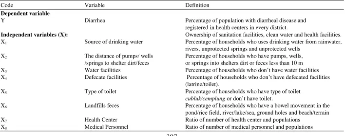
Table 1: Variables
Code Variable Definition
Dependent variable
Y Diarrhea Percentage of population with diarrheal disease and registered in health centers in every district.
Independent variables (X): Ownership of sanitation facilities, clean water and health facilities. X1 Source of drinking water Percentage of households who uses drinking water from rainwater,
rivers, unprotected springs and unprotected wells X2 The distance of pumps/ wells Percentage of households who have pumps, wells,
/springs to shelter dirt/feces or springs into shelters dirt or feces less than 10 m X3 Water facilities Percentage of households who don’t have water facilities
X4 Defecate facilities Percentage of households who don’t have defecated facilities
(latrine/toilet).
X5 Type of toilet Percentage of households who have type of toilet
cubluk/cemplung or don’t have toilet.
X6 Landfills feces Percentage of households who have a bowel movement in the
pond/rice field, river/lake/sea, ground holes and beach/terrain X7 Health Center Ratio of number of health center and populations
398 The formula of hypothesis test is Eq. 1:
o I I Z var(I) − = (1) Where: n n
ij i j
i 1 j 1
n n n
2
ij j
i 1 j 1 i 1
w (x x)(x x) n
I
w (x x)
= = = = = − − = −
∑∑
∑∑
∑
o 1 E(I) I n 1 = = − −Var (I) is the variance of Moran’s I and E (I) is the expected value. Reject Ho and there is a spatial autocorrelation if |Z|>Zα/2. The value of Moran’s I is
between -1 and 1. Value I> Io is shows the positive autocorrelation and I<Io is shows the neagtive autocorrelation.
Spatial durbin model: General model of Spatial Autoregressive (SAR) is shown in Eq. 2 and 3 (LeSage, 1999; Anselin, 1988):
y = ρW1y + Xβ + u (2)
And:
u = λW2u +ε (3)
ε ~ N(0,σ2I)
where, yrepresent vector of dependent variable (n×1), Xrepresent matrix of independent variable (n × (k+1)), β represent vector of regression coefficient parameter ((k+1) ×1), ρ represent spatial lag coefficient parameter on dependent variable, λ represent spatial lag coefficient parameter on error u and ε error (n×1), W1 and W2 represent weighted matrix (n×n), I represent identity matrix (n×n), n represent number of observations or locations (i = 1,2,3,...,n) and k represent number of independent variable (k = 1,2,3,...,l).
If X = 0 and W2 = 0, Equation 2 would be first order spatial autoregressive model y = ρW1y + ε. This model represents the variance on y as linear combination of variance among neighboring locations without independent variable. If W2 = 0 or λ = 0, Equation 2 would be Mixed Regressive-Autoregressive model or Spatial Autoregressive Model (SAR) y = ρW1y + Xβ + ε. This model assumed that autoregressive process just on dependent variable.
If W1 = 0 or ρ = 0, Eq. 2 would be Spatial Error Model (SEM) y = Xβ + λW2u+ε. λW2u is represents structure spatial λW2 on spatially dependent error (ε). When W1, W2≠0, λ≠0, or ρ ≠ 0 Eq. 2 is called Spatial Autoregressive Moving Average (SARMA). Then, if ρ
= 0 and λ = 0 Equation 2 is called linear regression y = Xβ + ε, which don’t spatial effect.
Spatial Durbin Model (SDM) is special cases of SAR, which adding spatial lag on independent variable (Anselin, 1988). This model was developed because the dependencies in the spatial relationships not only occur in the dependent variable, but also in the independent variable. SDM model is show in Eq. 4:
1 o 1 1 2
y= ρW y+ β + β +X W Xβ + ε (4) Vector coefficient parameter of spatial lag on independent variable is 2 β.
Model Eq. 4 can be formed into Eq. 5 and 6:
1 1
1 2
1
y (I W ) Z
y ~ N((I W ) Z , I) −
−
= − ρ β + ε
− ρ β σ (5)
Where:
Z = [I X WX] β = [β0, β1, β2]T (6) Parameter estimation of SDM can be performing by Maximum Likelihood Estimation (MLE). It was reference from Ord (1975); Anselin (1988); Arbia (2006); Mur and Angulo (2006) and also LeSage and Pace (2009).
RESULTS
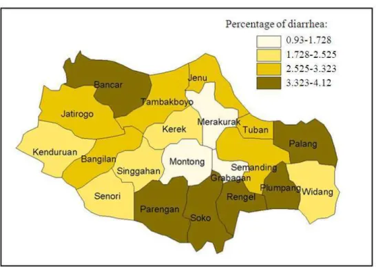
In 2007, the population of Tuban Regency was 1,127,416 persons with the population density of 613 persons per km2. Health Department noted that there are 2.82% or 31.770 persons who suffering diarrhea. Compared to regencies in East Java, Tuban Regency was ranked the ninth to the incidence of diarrhea. That number has declined over the previous year. It shows from 2.84% or 31 917 persons who suffer diarrhea.
399
Fig. 1: Percentage of Diarrhea in Tuban Regency 2007 Source: Health Center, 2007
Table 2:Moran’s I test
Variables Moran’s I Zscore
Diarrhea (Y) 0,015 0,514
Source of drinking water (X1) 0,052 1,705**
The distance of pumps/wells/springs 0,178 1,896** to shelter dirt/feces(X2)
Water facilities (X3) 0,005 0,446
Defecate facilities (X4) 0,165 1,650**
Type of toilet (X5) 0,171 1,654**
Landfills feces (X6) 0,405 3,446*
Health Center (X7) -0,131 -0,557
Medical Personnel (X8) 0,053 0,836
Note: (*) significant at α = 5%, (**) significant at α = 10% Z0,025=
1,96, Z0,05 = 1,64
The distributions of other variables are presented in Fig. 2. The figure also shows that there were clustered sub district that have same characteristics. Sub districts which have high percentage of households who have type of toilet cubluk or cemplung or don’t have toilet were in north area (Fig. 2d). There were Jatirogo, Bancar and Jenu which have 68.492-90.63%. Then, sub districts in middle area have lower percentage than other.
Moran’s I: The result of spatial autocorrelation test was shown in Table 2. The result of spatial autocorrelation test was landfills feces variables (X6) have autocorrelation among sub districts at level significant 5%. The results at level significant 10%
were source of drinking variable (X1), the distance of pumps/wells/springs to shelter dirt/feces variable (X2), defecate facilities (X4) and type of toilet (X5) have autocorrelation among sub districts. It showed from the value Z score which exceed Z0,025 = 1,96 and Z0,05 = 1,64.
Most of the independent variable have the value of Moran’s I greater than Io = -0.053. It indicates that there was positive autocorrelation or clustered data pattern. Sub districts which in the some cluster have similar characteristics. The diarrhea incidence as the dependent variable has Moran’s I of 0.015 which was not significant both at α = 5% and 10%. Based on comparison by Io, it indicates that the data pattern is spread. Among sub districts have different characteristics of diarrhea. Other variables that have a pattern of spread were water facilities (X3), health center (X7), medical personnel (X8).
400 independent variable in model. Furthermore, testing on residual assumption, residual were normally distributed
and independent, but not identic or heterodeskedasitas. Parameter estimation on SDM is presented on Table 4.
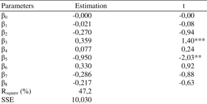
401 Table 3:Parameters estimation by OLS
Parameters Estimation t
β0 -0,000 -0,00
β1 -0,021 -0,08
β2 -0,270 -0,94
β3 0,359 1,40***
β4 0,077 0,24
β5 -0,950 -2,03**
β6 0,330 0,92
β7 -0,286 -0,88
β8 -0,217 -0,63
Rsquare (%) 47,2
SSE 10,030
Note: (*) significant at α = 10%, (**) significant at α = 20%, n = 20
τ0, 95; 11 1,796, τ0,9;11 = 1,363
Table 4: Parameter estimation by SDM
Parameters Estimation Wald
β0 0.3296 3.1280**
β11 0.6468 3.3371**
β12 -0.4006 3.3434**
β13 0.7229 15.2629*
β14 0.1010 0.1294
β15 -0.4729 1.5849
β16 -0.3522 0.7819
β17 0.6351 3.1593**
β18 -0.7977 7.9760*
β21 2.3123 4.8657*
β22 -1.1092 3.5350**
β23 0.9243 0.5276
β24 0.1932 0.1202
β25 -0.5305 0.1142
β26 -1.6347 2.6102***
β27 2.1869 3.8805*
β28 -2.3712 7.9906*
ρ -0.4293 1.8221***
Rsquare(%) 66,06
SSE 5.9743
Note: (*) significant at α = 5%, (**) significant at α = 10%, (***) significant at α = 20%, n = 20 χ20,05;1 = 3841, χ20,10;1 = 2,706,
χ20,20;1 = 1,642
DISCUSSION
The pattern of diarrhea distribution was clustered and similar characteristics among nearby locations showed that the spatial analysis needs to ρ be done. Furthermore, moran’s I show that there were a spatial autocorrelation in some variable.
OLS method has poor performance, because the assumption of identical residual not met. Not identic would effect on residual variances which was not homogeneous. It indications that residual was clustered. Therefore it was necessary for spatial modeling.
The result of SDM was that there was dependency lag on dependen and independent variable. It was shown by parameter ρ and β2 which significant effect. The significance of the lagged independent variable was indicated by the independent variables with weighting which significant effect to model. These variables were source of drinking water, health center
and medical personnel which were significant at α = 5%. Other variables which were significant at α = 20% were the distance of pumps/wells/springs to shelter dirt/feces and landfills feces. Coefficient determinansi is 66.06% and sum square error is 5.9743.
Coefficient of weighted sources of drinking water variable was 2.3123. It is positive value. It indicates sub district, which was nearby with other sub districts by the high percentage of households who used drinking water from rain water, rivers, unprotected springs and unprotected wells, will has high percentage of diarrheal disease. Otherwise, sub district, which was nearby with other sub districts by the low percentage households who uses drinking water from rain water, rivers, unprotected springs and unprotected wells, will has low diarrheal disease.
Model comparison of OLS and SDM showed that SDM was given better performance than OLS. It has sum square error smaller and there were many parameters which significant effect on model. Based on the analysis, it can be concluded that the lagged dependent and independent variable is very important about the role of modeling the diarrhea and the factors that influence it. Furthermore, based on the relationship between the incidence of diarrhea and ownership of sanitation, water and health facilities, the similarities or differences in the characteristics many sub districts may result an increase or decrease the diarrhea incidence. Example, sub district which have high percentage of households uses a source of drinking water from springs and wells unprotected will be triggered by a nearby districts which have low percentage incidence of diarrhea. These triggers can be done by the relevant programs which have been implemented by government.
CONCLUSION
Diarrhea case in Tuban Regency has spatial effect. It can be shown from Morans’I and SDM of diarrhea incidence and factors that influence it. The results of SDM show that the lag in the dependent and independent variables significantly affected. These independent variables were source of drinking water, health center and medical personnel which were significant at α = 5%. Furthermore, SDM was give better performance than OLS. It has sum square error smaller and there were many parameters which significant effect on model. In SDM model, lag on dependent and some independent variable.
ACKNOWLEDGEMENT
402
REFERENCES
Anselin, L., 1988. Spatial Econometrics: Methods and Models. Ist Edn., Kluwer Academic Publishers, Netherlands, ISBN-10: 9024737354, pp: 304. Arbia, G., 2006. Spatial Econometrics: Statistical
Foundations and Applications to Regional Convergence. 1st Edn., Springer,Berlin Heidelberg New York, ISBN-10: 354032304X, pp: 208. Arumsari, N. and Sutikno, 2010. Modeling of Diarrhea
by Spatial Regression. Case Study: Tuban Regency, East Java Provincy. Proceedings of Seminar Nasional Pasca Sarjana X, Aug. 4-4, ITS Surabaya, pp: 6-31.
Bekti, R.D. and Sutikno, 2011. Spatial Modeling on the Relationship between asset society and poverty in East Java. J. Matematika Sains, 16: 140-146. Brasington, D.M. and D. Hite, 2005. Demand for
environmental quality: A spatial hedonic analysis. Regional Sci. Urban Econ., 35: 57-82. DOI: 10.1016/j.regsciurbeco.2003.09.001
Elobaid, R.M., M. Shitan, N.A. Ibrahim, A.N.A. Ghani and Daud, 2009. Evolution of spatial correlation of mean diameter: A case study of trees in natural Dipterocarp Forest. J. Math. Stat., 5: 267-269. DOI: 10.3844/jmssp.2009.267.269
Kazembe, L.N., A.S. Muula and C. Simoonga, 2009. Joint spatial modelling of common morbidities of childhood fever and Diarrhoea in Malawi. Health
Place, 15: 165-172. DOI:
10.1016/j.healthplace.2008.03.009
Kissling, W.D. and G. Carl, 2007. Spatial autocorrelation and the selection of simultaneous autoregressive models. Global Ecol. Biogeography, 17: 59-71. DOI: 10.1111/j.1466-8238.2007.00334.x
Lee, J. and D.W.S. Wong, 2001. Statistical Analysis with ArcView GIS. Ist Edn., John Wiley and Sons, New York, ISBN-10: 047143776X, pp: 208. LeSage, J.P. and R.K. Pace, 2009. Introduction to
Spatial Econometrics. 1st Edn., Taylor and Francis, Boca Raton, ISBN-10: 142006424X, pp: 340. LeSage, J.P., 1999. The theory and practice of spatial
econometrics. University of Toledo.
Mur, J. and A. Angulo, 2006. The spatial Durbin model and the common factor tests. Spatial Econ. Anal., 1: 207-226. DOI: 10.1080/17421770601009841 Murad, A.A., 2011. Creating a geographical
information systems-based spatial profile for exploring health services supply and demand. Am. J. Applied Sci., 8: 644-651. DOI: 10.3844/ajassp.2011.644.651
Myaux, J., M. Ali, A. Felsenstein, J. Chakraborty and A.D. Francisco, 1997. Spatial distribution of watery diarrhoea in children: Identification of “Risk Areas” in a rural community in Bangladesh. Health Place, 3: 181-186. DOI: 10.1016/S1353-8292(97)00013-0
Ord, K., 1975. Estimation methods for models of spatial interaction. J. Am. Stat. Assoc., 70: 120-126. DOI: 10.1080/01621459.1975.10480272