www.hydrol-earth-syst-sci.net/10/209/2006/ © Author(s) 2006. This work is licensed under a Creative Commons License.
Earth System
Sciences
Efficient reconstruction of dispersive dielectric profiles using time
domain reflectometry (TDR)
P. Leidenberger1, B. Oswald1,*, and K. Roth1
1Institute of Environmental Physics, University of Heidelberg, Heidelberg, Germany *now at: Paul Scherrer Institute, Villigen, Switzerland
Received: 29 July 2005 – Published in Hydrol. Earth Syst. Sci. Discuss.: 15 August 2005 Revised: 20 January 2006 – Accepted: 10 February 2006 – Published: 11 April 2006
Abstract.We present a numerical model for time domain re-flectometry (TDR) signal propagation in dispersive dielectric materials. The numerical probe model is terminated with a parallel circuit, consisting of an ohmic resistor and an ideal capacitance. We derive analytical approximations for the ca-pacitance, the inductance and the conductance of three-wire probes. We couple the time domain model with global opti-mization in order to reconstruct water content profiles from TDR traces. For efficiently solving the inverse problem we use genetic algorithms combined with a hierarchical param-eterization. We investigate the performance of the method by reconstructing synthetically generated profiles. The algo-rithm is then applied to retrieve dielectric profiles from TDR traces measured in the field. We succeed in reconstructing dielectric and ohmic profiles where conventional methods, based on travel time extraction, fail.
1 Introduction
1.1 Motivation
Time Domain Reflectometry (TDR) has become an indis-pensable technique for measuring the water content of soils in hydrology, civil engineering, agriculture and related fields over the last years, for a review see Robinson et al. (2003). Early realizations of the method delivered a single water con-tentθ from a TDR trace (Birchak et al., 1974; Topp et al., 1980, 1982a,b; Topp and Davis, 1985; Dasberg and Dalton, 1985). A second phase of TDR development has targeted to deliver spatially resolved water content profiles along the TDR probe (Yanuka et al., 1988; Hook et al., 1992; Das-berg and Hopmans, 1992; Lundstedt and Str¨om, 1996; Nor-gren and He, 1996; Pereira, 1997; Todoroff et al., 1998; Feng
Correspondence to:B. Oswald ([email protected])
et al., 1999; Oswald, 2000; Oswald et al., 2003; Lin, 2003; Heimovaara et al., 2004; Schlaeger, 2005).
Because the dielectric permittivity of soil material typi-cally depends considerably on frequency, particularly if there are clay and loam components (Hoekstra and Delaney, 1974; Sposito and Prost, 1982; Ishida et al., 2000; Huisman et al., 2004; Robinson et al., 2005), in a third phase methods have been studied to recover the average dispersive dielectric pa-rameters from TDR traces (Heimovaara, 1994; Heimovaara et al., 1996; Hilhorst et al., 2001; Lin, 2003). Clearly, the next logical step are methods to extract the full dielectric pro-file from a TDR trace.
1.2 Objectives
In this paper we study an efficient method for the recon-struction of spatially resolved profiles of water content and electrical conductivity from TDR traces assuming disper-sive dielectric properties of the soil material along the probe. In particular, we want to reconstruct field measured TDR traces (Wollschl¨ager and Roth, 2005) which could not be suc-cessfully reconstructed with techniques used by Roth et al. (1990).
2 Methods
The propagation of TDR signals, voltagev (x, t) and cur-renti (x, t ), on probes of two or more conducting rods is de-scribed by transmission line theory (e.g. Ramo et al., 1984). Our approach for numerically modeling TDR probes is es-sentially based on Oswald et al. (2003). A transmission line is described by capacitanceC′, conductanceG′, induc-tanceL′ and resistanceR′, all per unit length, respectively. These parameters are functions of the probe geometry and the dielectric and ohmic properties of the material between the probe’s conductorsC′=C′(d, D, ǫ), G′=G′(d, D, σ ),
L′=L′(d, D, µ) and R′=R′(d, D, Rskin) where d is the spacing between the probe rods (for a three rod probe this is the distance between neighboring rods) andDis the diam-eter of the probe rods. We assume rods of identical diamdiam-eter. For piecewise constant transmission line parameters, volt-agev (x, t )and currenti (x, t )are described by the the fol-lowing two linear first order, partial differential equations (PDE) (Ramo et al., 1984):
∂v ∂x = −
R′+L′∂ ∂t
i (1)
∂i ∂x = −
G′+C′ ∂ ∂t
v. (2)
The piecewise constant dielectric permittivityǫ and ohmic conductivityσ can be discontinuous, because the water con-tent θ in general is discontinuous across soil boundaries. With a variable water contentθ (x)along the probe the pa-rameters G′ and C′ vary accordingly; L′ is assumed to be constant, because the materials’ magnetic permeability equalsµ0; resistanceR′, caused by skin effect, is neglected in the current study.
For extracting dielectric and ohmic profiles from measured TDR traces we use an iterative, globally optimizing approach based on Oswald et al. (2003) in order to solve the non-linear, inverse, electromagnetic problem. The global optimization method uses genetic algorithms (GA) from a publicly avail-able library Levine (1996).
To calculate the TDR signal for a given dielectric profile we numerically solve Eqs. (1) and (2) using a finite difference time domain (FDTD) approach (Taflove, 1998). The spatial discretization of thex coordinate is given by x=k1x and temporal discretization byt=n1twith:
1x≤ λmin
10 (3)
whereλminis the minimum wavelength present in the sys-tem, which in non-magnetic material, is determined by the maximum frequencyfmaxand the largest permittivity value
ǫmax(Taflove, 1998):
λmin=
c0
fmax√ǫr,max
. (4)
We estimate the maximum relevant frequency from
trise·f3 dB=0.34, (5)
an expression widely used in electrical engineering. It refers to a Gaussian type time domain waveform with rise timetrise. This is a good model for a TDR input signal.
To keep the explicit time domain integration scheme sta-ble, an upper limit for1t must be observed (Taflove, 1998; Kunz and Luebbers, 1993):
1t ≤ 1x c0
(6) 2.1 Numerical solution of transmission line equations Numerically, there are three spatially different regions, at the beginning of the probe x=0, at the end of the probe,
x=3, and in-between,x<0<3. At the ends of the probe, the discretized set of PDE is connected to a lumped elec-trical model, such as voltage sources or resistive-capacitive terminations.
2.1.1 Boundary conditions
The termination of a TDR probe is modeled with a parallel circuit, consisting of an ohmic resistor and an ideal capaci-tance. The voltage current relationship of this parallel circuit is given by
IT =
VT
RT +
CT
∂VT
∂t (7)
whereIT is the current at the end of the TDR probe through
the terminal resistor RT and the terminal capacitance CT.
VT is the voltage drop at the end of the TDR probe over the
parallel circuit ofRT andCT. To couple this parallel circuit
to the distributed transmission line model we use Eq. (1). We truncate the FDTD scheme of the probe through coupling Eqs. (1) and (7) using the definitions:
i (x=3, t )=IT (8)
v (x=3, t )=VT. (9)
We rewrite Eq. (1)
∂v ∂x = −R
′
ki−L′k
∂i ∂t
x
=3
(10)
⇒∂x∂ v (x=3, t )= −RK′ i (3, t )−L′K ∂
∂ti (3, t ) . (11)
All current terms in Eq. (11) are replaced by inserting Eq. (7). Note that the currents in the expressions, both constitutive and first-order PDE, are equivalent. Also, the voltages at the end of the probe and across the resistor are equal:
∂
∂xv (3, t )= − RK′ RT
v (3, t )−R′KCT
∂
∂tv (3, t) −L
′
K
RT
∂
∂tv (3, t )−L ′
KCT
∂2
We select a suitable discretization of Eq. (12): (i) the dis-cretization must result in a fully explicit update scheme; (ii) the scheme must not require values outside the spatial com-putational domainx=[0. . . 3]. We choose the “backward differencing in space” and “forward differencing in time” scheme using the Taylor series expansion of first-order accu-racy. The sum of backward and forward second-order Tay-lor series expansion in time provides the second order time derivative. With the usual notation we write the discretized version of Eq. (12):
vn
K−v
n K−1
1x
= −R
′
K
RT
vnK−RK′ CT
vKn+1−vnK 1t
!
−L ′
K
RT
vKn+1−vnK 1t
!
−L′KCT
vKn+1−2vKn +vKn−1 1t2
!
. (13)
Finally, by rearranging Eq. (13) we obtain the explicit update procedure, in the time domain, for the voltage at the end of the TDR probex=3.
vKn+1=
R′
KCT
1t +
L′K RT1t +
L′KCT
1t2 −1
·
vKn
2L′KCT
1t2 +
L′K RT1t +
RK′ CT
1t −
R′K RT
−1x1
−L ′
KCT
1t2 v
n−1
K +
1
1xv
n K−1
(14)
and similarly for the current atx=3from, using Eq. (7):
iKn+1= 1 RT
vKn+1+CT
vnK+1−vKn
1t . (15)
As special cases we mention CT=0, RT<∞ and CT=0,
RT→∞. An overview of the equations of all these boundary
conditions is given in Table 1. We have implemented them in our TDR code, so almost any given experimental setup can be modeled. The values ofCT andRT can also be optimized
for, if so desired.
To implement the excitation we employ the same approach used by Oswald et al. (2003). We couple a resistive voltage source to the distributed transmission line. The resistive volt-age source consists of a series of an ideal ohmic resistorRS
and an ideal voltage sourcevnS. To avoid reflections between the voltage source and the cable connecting the TDR instru-ment to the probe we adjustRS to the impedance of the
con-necting cable. The current flow out of the resistive voltage source isiSn. The time derivative of the source voltage is im-plemented with a discretized version of the given expression for the time domain signal shape.
Fig. 1.Three-rod probe configuration and parameters.
2.1.2 Transmission line parameters for three-rod TDR probe
To solve the forward TDR problem the transmission line parameters for the three-rod probe, C′,G′, L′ and R′, are essential. Closed-form, analytical expressions for the two-rod probe and the coaxial line are well known (Ramo et al., 1984). This is however not the case for the three-rod probe. We will derive an analytical model for the three-rod TDR probe based on an approximation of the electric and mag-netic fields. The resulting transmission line parameters are compared to numerical simulations.
We calculate the electric parameters,C′andG′, from the
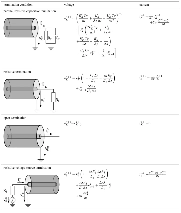
Table 1.Summary of boundary conditions.
termination condition voltage current
parallel resistive capacitive termination
vKn+1= R
′
KCT
1t + L′K RT1t +
L′KCT
1t2
!−1
·
"
vKn 2L ′
KCT
1t2 + L′K RT1t
+R
′
KCT
1t − RK′ RT −
1 1x
!
− L
′
KCT
1t2 v
n−1
K +
1 1xv
n K−1
#
iKn+1=R1TvnK+1
+CT vKn+1−vKn
1t
resistive termination
vKn+1=vnK 1−R
′
K1t
L′K − 1t RT L′K1x
!
+vKn −1
1t RT
L′K1x
ikn+1= R1TvKn+1
open termination
vKn+1=vKn+1
−1 i
n+1
K =0
resistive voltage source termination
vkn+1=vnk 1−1t R
′
1 L′1
1t RS
L′11x
!
+1t RS
L′11xv
n k+1+
1t R1′ L′1 v
n S
+1t∂v
n S
∂t
i1n+1=v
n+1 S (t )−v
n+1 1
RS
a specific conductor. The details of the derivation are given in Appendix A. The electrostatic potential, magnetic field, and the geometrical basis of the three-rod probe for
Table 2.Fit functions and parameters for numerical extracted transmission line parameters for a three rod probe. The fit functions following the structure of Eqs. (16)–(18). Validated forκ=1.5. . .40.
fit function a b c d e f g
C(κ)= b aπ ǫ
+ln(cκ+d)+eln(f κ+g)
G(κ)= aπ σ
b+ln(cκ+d)+eln(f κ+g)
9.758·10+1 1.090 9.486·10+1 −1.421·10+2 7.516·10+1 1.278 3.772·10−1
L(κ)= aµπ (b+ln(cκ+d)
+eln(f κ+g)) 7.692·10−
3 7.857·10−1 7.654·10+1 −1.147·10+2 9.846·10+1 1.395 2.592·10−1
0 5 10 15 20 25
0 1 2 3 G’ [S/m]
κ [−] numerical simulation fit
analytic approximation
0 5 10 15 20 25
-20 -10 0 10 20 30 40
relative deviation [%] κ [−]
simulation to fit analytic approx. to fit
Fig. 2. Comparison of numerical and analytical extracted conduc-tance per unit lengthG′for a three-rod probe as a function of probe geometryκ=Dd;σ=0.5. Top: transmission line parameter from: (i) numerical simulations and a fit through them, Table 2; (ii) analyti-cal approximation, Eq. (17). Bottom: relative deviation of the: (i) numerical results to the fit; (ii) approximative model forG′to the fit.
κ=Dd are then obtained as
C′= 4π ǫ
ln44κκ2−−11+2 ln(2κ−1)
(16)
G′= 4π σ
ln44κκ2−−11+2 ln(2κ−1)
(17)
L′= 3µ0
4π
ln(2κ−1)+1
3ln
2κ+1 4κ−1
. (18)
For assessing the quality of the approximate solutions we use the commercially available 3-dimensional electrodynamics
0 5 10 15 20 25
0 2.0e-7 4.0e-7 6.0e-7 8.0e-7 1.0e-6 1.2e-6 1.4e-6 1.6e-6 L’ [H/m]
κ [−] numerical simulation fit
analytic approximation
0 5 10 15 20 25
-30 -20 -10 0 10 20
relative deviation [%]
κ [−]
simulation to fit analytic approx. to fit
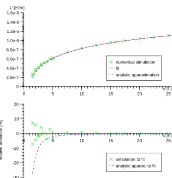
Fig. 3. Comparison of numerical and analytical extracted induc-tance per unit lengthL′for a three-rod probe as a function of probe geometryκ=Dd. Top: transmission line parameter from: (i) nu-merical simulations and a fit through them, Table 2; (ii) analytical approximation, Eq. (18);µr=1. Bottom: relative deviation of the:
(i) numerical results to the fit; (ii) approximative model forL′to the fit.
solver HFSS™ from Ansoft Inc. First, we determined the transmission line parameters for a two rod probe. The dif-ferences between the numerical values and the exact solution are less than 1%. We then numerically evaluate the transmis-sion line parameters of a three-rod probe using HFSS and fit them to an appropriately parameterized function. The re-sults of the analytical model and the numerical simulations are shown in Figs. 2–3. Table 2 presents the used fit func-tions and their corresponding parameters.
computation time increase considerably. Forκ>5 we get an excellent agreement between the analytic approximation and the heuristic fit basing on the numerical simulation. Forκ≤5 the analytic approximation becomes inaccurate and the nu-meric simulation starts to oscillate. This is a problem of the discretization and can be alleviated by using a machine with more memory.
Calculating the propagation velocity with the fit functions forL′andC′, viac=√1
L′C′, the maximum relative deviation of the speed of lightc0is 0.14% overκ=1.5. . .25. For the two three rod TDR probes we useκ is 4.69 and 6.25 so we get an error in speed of lightc0of 0.12% and 0.13%. The quality of the analytical model improves with increasingκ, corresponding more and more to the situation of infinitely thin line charges and current filaments, respectively.
2.2 Time domain dispersive dielectric modeling
Experience gained from TDR traces measured in the field has shown that it is mandatory to consider dispersive di-electric soil properties. We start with a Debye model using one single relaxation frequency (Debye, 1929; Nyfors and Vainikainen, 1989; Taflove, 1998). The Debye model de-scribes the orientation polarization of polar molecules. Let us think of an electric field, switched on instantaneously. The polar molecules turn and the polarization evolves exponen-tially, with a time constantτ, to its final state. The relative dielectric permittivityǫras a function of frequency is then:
ǫr(ω)=ǫ′∞+
ǫ′
s−ǫ′∞
1+j ωτ. (19)
Hereǫ∞′ is the permittivity at infinite frequency, where the orientation polarization of the molecules has no time to de-velop. The static permittivityǫ′
s corresponds to a state where
the orientation polarization has had sufficient time to develop fully. For solving the transmission line equations in the time domain, we transform Eq. (19) into the time domain.
ǫr(t )=ǫ∞′ δ (t)+
1ǫ′ τ e
−τtU (t ) (20)
with1ǫ′r=ǫs′−ǫ∞′ . We end up with a time-dependent ca-pacitance per unit lengthC′(t ), which is split into a time-dependent and a time-intime-dependent part:
C′(t )=C0′ǫr(t ) (21)
Equation (21) with Eqs. (2) and (1) are discretized, using central finite differences both in space and in time. We obtain the update procedure for the voltage and current:
vkn+1= −21t G ′
k
C′
0kǫ∞′ k
vnk −21t 1ǫ ′
k
ǫ′ ∞kτk
vnk+vnk−1
−C′ 1t 0kǫ∞′ k1x
ikn+1−ikn−1 +21ǫ
′
k1t
τk2ǫ′ ∞k
ψkn (22)
ink+1= −2R ′
k1t
L′k i
n k +i
n−1
k −
1t 1xL′k v
n
k+1−vkn−1
(23) with the abbreviation
ψkn=e− 1t
τkψkn−1+1t
2
vkn+e− 1t τkvnk−1
. (24)
The detailed calculation for this discretization can be found in Appendix B.
2.3 Hierarchical optimization
Our profile reconstruction approach is based on Oswald et al. (2003). The non-linear inverse problem is solved iteratively with a transmission line solver to calculate TDR traces, based on a given profile of electric parameters. The forward solver is embedded into a global optimizer based on a genetic algo-rithm (Levine, 1996; Rahmat-Samii and Michielssen, 1999) which delivers electric parameter profiles, adapted accord-ing to their fitness. Fitness is a quantity which is roughly inversely proportional to the trace mismatch:
m=
Nstop X
n=Nstart
|vmeas(n1t )−vcalc(n1t )|, (25)
We use the sum of absolute values of the difference between calculated and measured TDR traces in contrast to the sum of squared differences (Oswald et al., 2003) because it is a robust estimator, typically used for non-Gaussian errors. In contrast the sum of squared differences, theL2-norm, is only applicable to Gaussian noise. The genetic algorithm operates on bit-strings which are mapped to real numbers to produce the electric parameter profiles. Hence the electric parameters are inherently discretized. Using a sufficient number of bits per parameter we provide a fine-grained set of values. The efficiency of profile reconstruction depends on the genetic algorithm’s parameters: mutation rate, crossover probability and population size. The corresponding values are listed in Tables 4 and 6.
While Oswald et al. (2003) achieve to solve the problem, there are still issues, namely (i) it is computationally inten-sive due to a large number of forward problem runs and (ii) the resulting electric parameter profiles may exhibit os-cillatory behavior even if their average corresponds to the converged state.
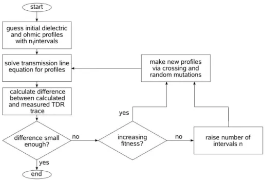
To reduce the computational burden and to achieve smoother parameter profiles we have implemented a hierar-chical optimization scheme (Fig. 4). The scheme starts out with a coarse spatial resolution which is increased as con-vergence rate decreases. For assessing the degree of conver-gence we calculate the envelope of the fitness and approxi-mate its slope with a line (Fig. 5). An envelope point (squares at green line) is retrieved as the maximum fitness value ofN
consecutive individuals, in our caseN=30. A complete en-velope consists ofM such points. As soon as the next N
Fig. 4.Flowchart for the hierarchical optimization.
Table 3.Parameters used for calculation of synthetic TDR traces for validation and demonstration of termination conditions and the disper-sive media, for all: probe length=0.1 m, TDR rise timetrise=300 ps,κ=10, conductor diameterD=4 mm.
Figure number ǫ′∞ 1ǫ′ frel(MHz) σ′
S m
RT () CT (F) tsec 1x (m)
6 10 – – 1·10−30 – – 0.25 1.2·10−3
7 1 – – 1·10−30 1438.8 5.0·10−12 0.10 5.0·10−4
9 10 10 100 1·10−30 – – 0.25 1.2·10−3
8 (green line) 10 – – 1·10−30 113 – 0.20 1.0·10−3
8 (red dotted line) 10 – – 1·10−30 1436.8 5·10−12 0.20 1.0·10−3
8 (blue dashed line) 10 – – 4·10−2 – – 0.20 1.0·10−3
10 (green line) 10 10 10 1·10−30 – – 0.20 1.0·10−3
10 (red dotted line) 10 5 100 1·10−30 – – 0.20 1.0·10−3
10 (blue dashed line) 10 10 100 1·10−30 – – 0.20 1.0·10−3
discarded and the whole envelope section is moved one point ahead with respect to the sequence of evaluated individuals. If the majority of envelope points is below the line (red line), with the slope defined in the job file, the spatial resolution is increased by cutting the intervals of dielectric properties into halves. The new intervals are initialized with the same dielectric properties, as the old intervals had at the same loca-tion. The optimization stops if a previously specified spatial resolution is reached and the fitness does not increase.
3 Results
3.1 Validation of parallel RC boundary condition
We show the results of TDR traces calculated for different probe termination conditions with a non-dispersive dielectric permittivity between the probe conductors, for all parameters cf. Table 3. Figure 6 shows a comparison for the open termi-nation, calculated with HFSS™ and our own code. All traces generated with HFSS™ were calculated under the assump-tions (i) that the TDR signal source is connected directly to the probe and (ii) that the source has the same impedance as the probe. Therefore, there is no initial reflection.
Fig. 5.Determination of the criteria when to increment spatial res-olution.
0 1.0 2.0 3.0 4.0 5.0 6.0 7.0 8.0 9.0 10.0
0 0.25 0.50 0.75 1.00
ρ
time [ns] our code HFSS
Fig. 6.Calculated TDR trace with HFSS (blue dashed line) and our code (green line) for two-rod probe with lengthl=0.1 m,D=4 mm, κ=10,ǫ∞′ =10,σ=10−30S/m, not dispersive, infinite termination.
and are not a pure result of numeric simulation. We calcu-late the TDR probe fully 3-dimensional with HFSS™ so it includes the finite length of the transmission line. Our code uses the ideal transmission line equations, only valid for in-finite long transmission lines. The influence of this effect is important in the content of spatial reconstruction of dielectric profiles. We expect a higher systematic error for the recon-structed dielectric parameters at the end of the probe, than for the rest.
Figure 7 shows the result of a probe with parallel resistive capacitive termination. At the reflection we can see the effect of the resistive capacitive termination: (i) in the beginning it behaves like a short circuit; (ii) if the capacitor is completely charged, it behaves like a pure resistive termination; (iii) and the edges of the reflections are smoothed. In Fig. 8 differ-ent termination conditions are calculated with our code. The TDR source here has an impedance of 50, therefore the first reflection results from the source-probe-transition, the second from the end of the probe. After these, there are mul-tiple reflections. The TDR probe terminated with the probe’s impedance produces the green trace. There are no reflections resulting from the end of the probe, as expected. The red
0 1.0 2.0 3.0 4.0 5.0
-0.75 -0.50 -0.25 0 0.25 0.50
ρ
time [ns]
our code HFSS
Fig. 7.Calculated TDR trace with HFSS (blue dashed line) and our code (green line) for two-rod probe with lengthl=0.1 m,D=4 mm, κ=10,ǫ∞′ =1,σ=10−30S/m, not dispersive, parallel resistive ca-pacitive termination,RT=1436.8,CT=5.0·10−12F.
0 1.0 2.0 3.0 4.0 5.0 6.0 7.0 8.0 9.0 10.0
0 0.25 0.50 0.75 1.00 1.25
ρ
time [ns] σ=10 S/m, R =113.0 -30 T Ω
σ=10 S/m, R =1436.8 , C =5*10 F-30 T Ω T -12
σ=4*10 S/m-2
Fig. 8. Calculated TDR trace with our code for two-rod probe with length l=0.1 m, D=4 mm, κ=10, ǫ∞′ =10, not dispersive: (i) (green line)σ=10−30S/m, resistive termination,RT=113;
(ii) (blue dashed line) σ=10−30S/m, parallel resistive capaci-tive termination,RT=1436.8,CT=5·10−12F; (iii) (red dashed
line) σ=4·10−2S/m, infinite termination. The discontinuity of impedance form TDR source to the probe causes the reflection at 0.3 ns.
dotted TDR trace demonstrates the effect of ohmic conduc-tivity between the probe conductors with an open terminated probe.
3.2 Validation of dispersive dielectric TDR model
Table 4.Parameters used for hierarchical TDR trace reconstruction of laboratory traces.
optimization parameter value to Figs. 12–14 value to Fig. 15
population size 50 50
crossover probability 0.6 0.05
mutation probability 0.01 0.01
bits forǫr′/ǫ∞′ 20 20
bits for1ǫ′ – 20
bits forfrel – 20
bits for conductivity 20 20
bits for terminal resistor – 10
bits for terminal capacitor – −
transmission line termination resistive resistive, optimized
termination resistor 214 786.9
TDR rise timetrise 28 ps 30 ps
spatial discretization 0.0005 m 0.001 m
time step security 0.9 0.25
TDR probe type two rod three rod
probe length 1.0 m 0.2 m
conductor diameterD 10.0 mm 4.0 mm
conductor center distanced 30.8 mm 25.0 mm
κ 3.08 6.25
0 1.0 2.0 3.0 4.0 5.0 6.0 7.0 8.0 9.0 10.0
0 0.25 0.50 0.75 1.00
ρ
time [ns] our code HFSS
Fig. 9.Calculated TDR trace with HFSS (blue dashed line) and our code (green line) for two-rod probe with lengthl=0.1 m,D=4 mm, κ=10,ǫ′∞=10,σ=10−30S/m, infinite termination, dispersive me-dia with1ǫ′=10,frel=100 MHz.
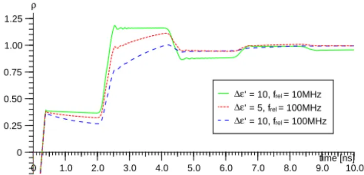
ohmic conductivity between the probe rods can be neglected; (ii) the reflections tend to smooth with the increasing effect of dispersion.
3.3 Hierarchical reconstruction of water content profiles 3.3.1 Traces measured in non-dispersive media
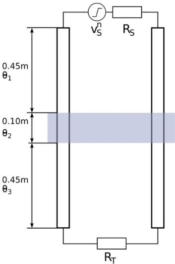
In Figs. 12–14 we show hierarchical reconstructions of the dielectric parameters for the same traces used by Oswald et al. (2003). The probe was in a sand tank with water con-tent θ1=θ3=0 and θ2 was varied. The experimental setup is sketched in Fig. 11. Relevant optimization parameters are given in Table 4. The vertical dashed lines in fitness and error
0 1.0 2.0 3.0 4.0 5.0 6.0 7.0 8.0 9.0 10.0
0 0.25 0.50 0.75 1.00 1.25
ρ
time [ns] ∆ε’ = 10, f = 10MHz’rel
∆ε’ = 5, f = 100MHz’rel
∆ε’ = 10, f = 100MHz’rel
Fig. 10.Calculated TDR trace with our code for two-rod probe with lengthl=0.1 m,D=4 mm,κ=10,ǫ∞′ =10,σ=10−30S/m, infinite termination and dispersion: (i) (green line)1ǫ′=10,frel=10 MHz; (ii) (red dotted line)1ǫ′=5,frel=100 MHz; (iii) (blue dashed line) 1ǫ′=10, frel=100 MHz. The discontinuity of impedance form TDR source to the probe causes the reflection at 0.3 ns.
history indicate an increase in spatial resolution. The number of spatial intervals are given in red in history and fitness.
Fig. 11. Experimental setup by Oswald et al. (2003): segmented sand tank with different water contents.
Table 5. Comparison of volumetric measured water content, per-mittivity of composite with Roth et al. (1990)’s model (α=0.5, ǫsoil=5,η=0.322) and the reconstructed relative dielectric permit-tivity corresponding to Fig. 15.
depth (cm) θ ǫc depth (cm) ǫr+1ǫ
volumetric reconstructed
0.0. . .2.5 4.32 0. . .4 0.001 3.41
2.5. . .5.0 3.99 5.0. . .7.5 3.95 5. . .9 0.001 3.41
7.5. . .10.0 4.33 10.0. . .12.5 8.72 10. . .14 0.022 4.06
12.5. . .15.0 11.31 15.0. . .17.5 12.44 15. . .19 0.224 13.18
17.5. . .20.0 12.16 20. . .24 0.322 19.48 – –
3.3.2 Traces measured in dispersive media
In Fig. 15 we show the hierarchical reconstruction of disper-sive dielectric parameters for a TDR trace, measured
verti-Table 6.Parameters used for hierarchical TDR trace reconstruction of field data.
TDR/optimization parameter value
population size 50
crossover probability 0.6 mutation probability 0.01
bits forǫ′∞ 20
bits for1ǫ′ 20
bits forfrel 20
bits for conductivity 20 bits for terminal resistor 10 bits for terminal capacitor 10
transmission line termination parallel resistive capacitive, optimized TDR rise timetrise 460 ps
measured samples 251
time between samples 107 ps spatial discretization 0.001 m
time step security 0.2
TDR probe type three rod
probe length 0.3 m
conductor diameterD 4.8 mm conductor center distanced 22.5 mm
κ 4.69 mm
cally in a sand tank. The probe ends in fully water saturated sand, while the sand at the probe head is dry. So we expect a strong gradient in the water content along the probe. We measure the water content volumetrically in different depths (probe head corresponds to z=0.0 m). If we compare the reconstructed dielectric parameters with volumetrically mea-sured parameters at Table 5, we see that they are in the same order; resistivity and permittivity increase in the longitudi-nal direction (for this comparison we use the relative dielec-tric permittivity ǫs′=ǫ∞′ +1ǫ′). Only the volumetric mea-surement at depth 10. . .14 cm and the reconstructed value at 10.0. . .12.5cm do not correspond. We denote that the differ-ent depths are not quite compatible: there is an uncertainty in the depth of the volumetric measurement and the TDR probe, is not calibrated.
In the discretized voltage update procedure, Eq. (22) the parameters describing the dispersion appear only as prod-ucts. If one of the reconstructed dispersion parametersfrel or1ǫ′approaches zero, the other dispersion parameter has
0 5000 0
2.0e+8 4.0e+8 6.0e+8 8.0e+8
1.0e+9 error of the individuals
[-]
individual [-]
1 2 4 8 16 32 64
0 5000
0 1 2 3
fitness of the individuals
[-]
individual [-]
1 2 4 8 16 32 64
0 2 4 6 8 10 12
0 0.25 0.50
0.75 measured TDR trace and calculated TDR trace ρ
time [nano sec.]
0 0.05 0.10 0.15 0.20 0.25 0.30 0.35 0.40 0.45 0.50 0.55 0.60 0.65 0.70 0.75 0.80 0.85 0.90 0
0.002 0.004 0.006
optimized absolute conductivity mean conductivity = 1.513223e-03 mS [mS/m]
probe length [m]
0 0.05 0.10 0.15 0.20 0.25 0.30 0.35 0.40 0.45 0.50 0.55 0.60 0.65 0.70 0.75 0.80 0.85 0.90 0
1 2
3 optimized relative permittivity mean permittivity = 2.717676e+00 [-]
probe length [m]
Fig. 12. Reconstruction of synthetic profile,θ2=0. Individual 7547 with error: 2.9·107and fitness: 3.4. Effective relative permittivityǫc
corresponding toθ2: (i) travel time evaluationǫc=2.78; (ii) Roth et al. (1990)’s modelǫc=2.49.
range of our TDR. It is not easy to extrapolate the relax-ation frequency very well and we get large errors for it with the frequency range of our TDR. Nevertheless the dispersion can not be neglected. Inclusion of dielectric dispersion is required to invert this TDR trace; reconstruction without dis-persion will inevitably fail.
3.3.3 Traces measured under field conditions
In Figs. 16–19 we show hierarchical reconstructions of TDR traces measured under field condition at the Grenzhof (Hei-delberg, Germany) test site (Wollschl¨ager and Roth, 2005). The traces were recorded with a “Campbell TDR 100” using a Campbell probe “CS610”. Essential TDR properties and the parameters used in the optimization to produce Figs. 16– 19 are shown in Table 6. The steps in all these measured traces result from finite time resolution in recording. The first reflection in all traces is a result of the TDR probe head. The head is simulated with a transmission line section.
Gen-erally, we can fit the transmission line parameters for this part with our simulation. Because the parameters are con-stant for every single probe, we fit them manually and fix the respective parameters in the job file, because it would unnec-essarily slow down the optimization if it was fitted for every trace from scratch once again. We particularly note Fig. 16. More conventional techniques (e.g. Roth et al., 1990) expe-rience severe problems, may even fail, to evaluate this trace, because there is no sharp reflection from the end of probe.
4 Discussion
0 5000 0
2.0e+8 4.0e+8 6.0e+8 8.0e+8
1.0e+9 error of the individuals
[-]
individual [-]
1 2 4 8 16 32 64
0 5000
0 1 2 3 4
fitness of the individuals
[-]
individual [-]
1 2 4 8 16 32 64
0 2 4 6 8 10 12
0 0.25 0.50
0.75 ρ measured TDR trace and calculated TDR trace
time [nano sec.]
0 0.05 0.10 0.15 0.20 0.25 0.30 0.35 0.40 0.45 0.50 0.55 0.60 0.65 0.70 0.75 0.80 0.85 0.90 0
0.002 0.004 0.006
optimized absolute conductivity mean conductivity = 1.303163e-03 mS [mS/m]
probe length [m]
0 0.05 0.10 0.15 0.20 0.25 0.30 0.35 0.40 0.45 0.50 0.55 0.60 0.65 0.70 0.75 0.80 0.85 0.90 0
1 2 3
optimized relative permittivity mean permittivity = 2.966710e+00 [-]
probe length [m]
Fig. 13.Reconstruction of synthetic profile,θ2=0.05. Individual 8146 with error: 2.3·107and fitness: 4.3. Effective relative permittivityǫc
corresponding toθ2: (i) travel time evaluationǫc=3.57; (ii) Roth et al. (1990)’s modelǫc=3.90.
commercial solver. We mention that the analytical model is most accurate for largerκ and becomes less accurate at very lowκ. This is caused by the fact that in the situation of large, closely spaced probe rods the electric and magnetic fields, obtained from the assumption of infinitely thin and infinitely extended line charges and current filaments, respectively, increasingly differ from the true fields. Nevertheless, it is remarkable how accurate its predictions are at largerκ.
We have validated our dispersive TDR code by comparing synthetically calculated traces from our code and HFSS™, for both dispersive and non-dispersive dielectric properties. We mention that dispersive dielectrics impose more strin-gent restrictions onto the time-step of the explicit integration scheme to keep it stable. This is related to the relative posi-tion of the dielectric relaxaposi-tion frequency and the dominant frequency content of the TDR signal source.
We have used a hierarchical approach to reconstruct elec-tric parameter profiles from TDR traces measured in the
0 5000 0
2.0e+8 4.0e+8 6.0e+8 8.0e+8
1.0e+9 error of the individuals
[-]
individual [-]
1 2 4 8 16 32 64
0 5000
0 1 2 3
fitness of the individuals
[-]
individual [-]
1 2 4 8 16 32 64
0 2 4 6 8 10 12
0 0.25 0.50
0.75 measured TDR trace and calculated TDR trace ρ
time [nano sec.]
0 0.05 0.10 0.15 0.20 0.25 0.30 0.35 0.40 0.45 0.50 0.55 0.60 0.65 0.70 0.75 0.80 0.85 0.90 0
0.005
optimized absolute conductivity mean conductivity = 2.921092e-03 mS [mS/m]
probe length [m]
0 0.05 0.10 0.15 0.20 0.25 0.30 0.35 0.40 0.45 0.50 0.55 0.60 0.65 0.70 0.75 0.80 0.85 0.90 0
2 4
optimized relative permittivity mean permittivity = 2.988377e+00 [-]
probe length [m]
Fig. 14.Reconstruction of synthetic profile,θ2=0.10. Individual 7977 with error: 2.7·107and fitness: 3.8. Effective relative permittivityǫc
corresponding toθ2: (i) travel time evaluationǫc=5.09; (ii) Roth et al. (1990)’s modelǫc=5.64.
Numerical experimentation for reconstructing TDR traces measured in the field has definitely shown that dispersive di-electric properties must be included in the numerical model. Only when using dispersive dielectrics can such TDR traces be recovered numerically; using frequency-independent per-mittivity alone can not account for the the shape of the traces. If the frequency range of the TDR instrument is well below the relaxation frequency, dispersion becomes less important. On the other hand, if the TDR’s frequency content and the relaxation frequency have a significant overlap, then disper-sion will be quite pronounced. The “Campbell TDR 100” has
f3 dB≈740 MHz. The relaxation frequencies extracted by the optimization are within this range and therefore dispersion is relevant (Robinson et al., 2003, 2005).
We note that in all cases we used a relatively small mu-tation probability, 0.01, and a significantly higher cross-over probability, 0.6. Increasing the mutation probability results in a more diverse population but does not seem to acceler-ate the convergence behavior. On the other hand, using a
relatively high cross-over probability ensures efficient recon-struction. The error and fitness histories represent the search in a wide parameter range. For some individuals we obtain a high error and a low fitness, respectively. The low fitness of some individuals give the black filled area in fitness history. Note that the error and fitness history are line plots. The high errors are cut off in the plots so that the relevant sector is vis-ible. Additionally, the error’s running average is plotted in the diagrams with a blue line.
0 20000 40000 0
2.0e+8 4.0e+8 6.0e+8 8.0e+8
1.0e+9 error of the individuals
[-]
individual [-]
1 2 4 8 9
0 20000 40000
0 5 10 15 20
fitness of the individuals
[-]
individual [-]
1 2 4 8 9
0 2 4 6 8 10
0 0.25 0.50 0.75 1.00
measured TDR trace and calculated TDR trace
ρ
time [nano sec.]
0 0.05 0.10 0.15 0.20
0
1 optimized absolute conductivity
mean conductivity = 1.934361e-01 mS [mS/m]
probe length [m]
0 0.05 0.10 0.15 0.20
0 5
optimized relative permittivity at infinite frequency mean permittivity at infinite frequency = 4.824102e+00 [-]
probe length [m]
0 0.05 0.10 0.15 0.20
0 5
optimized relative permittivity delta mean permittivity delta = 2.777455e+00 [-]
probe length [m]
0 0.05 0.10 0.15 0.20
2.0e+8 4.0e+8
optimized relaxation frequency mean relaxation frequency = 1.686587e+08 [Hz]
probe length [m]
0 10000 20000 0
2.0e+8 4.0e+8 6.0e+8 8.0e+8
1.0e+9 error of the individuals
[-]
individual [-]
1 2 4 8
0 10000 20000
0 10 20 30 40 50
fitness of the individuals
[-]
individual [-]
1 2 4 8
0 5 10 15 20 25
-0.25 0
measured TDR trace and calculated TDR trace
ρ
time [nano sec.]
0 0.05 0.10 0.15 0.20 0.25 0.30
0 20 40
optimized absolute conductivity mean conductivity = 4.493398e+01 mS [mS/m]
probe length [m]
0 0.05 0.10 0.15 0.20 0.25 0.30
0 10 20
optimized relative permittivity at infinite frequency mean permittivity at infinite frequency = 1.579151e+01 [-]
probe length [m]
0 0.05 0.10 0.15 0.20 0.25 0.30
0 5 10 15
optimized relative permittivity delta mean permittivity delta = 1.159271e+01 [-]
probe length [m]
0 0.05 0.10 0.15 0.20 0.25 0.30
1.0e+8 1.2e+8 1.4e+8
optimized relaxation frequency mean relaxation frequency = 1.127726e+08 [Hz]
probe length [m]
0 20000 0
2.0e+8 4.0e+8 6.0e+8 8.0e+8
1.0e+9 error of the individuals
[-]
individual [-]
1 2 4 8
0 20000
0 10 20 30 40 50
fitness of the individuals
[-]
individual [-]
1 2 4 8
0 5 10 15 20 25
-0.25 0 0.25
measured TDR trace and calculated TDR trace
ρ
time [nano sec.]
0 0.05 0.10 0.15 0.20 0.25 0.30
0 10 20
optimized absolute conductivity mean conductivity = 1.758309e+01 mS [mS/m]
probe length [m]
0 0.05 0.10 0.15 0.20 0.25 0.30
0 5 10
15 optimized relative permittivity at infinite frequency mean permittivity at infinite frequency = 1.163316e+01 [-]
probe length [m]
0 0.05 0.10 0.15 0.20 0.25 0.30
0 2 4
optimized relative permittivity delta mean permittivity delta = 2.359535e+00 [-]
probe length [m]
0 0.05 0.10 0.15 0.20 0.25 0.30
2.0e+8 4.0e+8
optimized relaxation frequency mean relaxation frequency = 1.832296e+08 [Hz]
probe length [m]
0 20000 0
2.0e+8 4.0e+8 6.0e+8 8.0e+8
1.0e+9 error of the individuals
[-]
individual [-]
1 2 4 8
0 20000
0 20 40 60 80
fitness of the individuals
[-]
individual [-]
1 2 4 8
0 5 10 15 20 25
0 0.25 0.50
measured TDR trace and calculated TDR trace
ρ
time [nano sec.]
0 0.05 0.10 0.15 0.20 0.25 0.30
0 1 2 3
optimized absolute conductivity mean conductivity = 2.076676e+00 mS [mS/m]
probe length [m]
0 0.05 0.10 0.15 0.20 0.25 0.30
0 5 10 15
optimized relative permittivity at infinite frequency mean permittivity at infinite frequency = 1.396445e+01 [-]
probe length [m]
0 0.05 0.10 0.15 0.20 0.25 0.30
0 5
optimized relative permittivity delta mean permittivity delta = 3.729491e+00 [-]
probe length [m]
0 0.05 0.10 0.15 0.20 0.25 0.30
1.0e+8 2.0e+8 3.0e+8
optimized relaxation frequency mean relaxation frequency = 1.475784e+08 [Hz]
probe length [m]
0 20000 0
2.0e+8 4.0e+8 6.0e+8 8.0e+8
1.0e+9 error of the individuals
[-]
individual [-]
1 2 4 8
0 20000
0 10 20 30 40
fitness of the individuals
[-]
individual [-]
1 2 4 8
0 5 10 15 20 25
0 0.25 0.50 0.75
measured TDR trace and calculated TDR trace
ρ
time [nano sec.]
0 0.05 0.10 0.15 0.20 0.25 0.30
0 1 2 3
optimized absolute conductivity mean conductivity = 1.281073e+00 mS [mS/m]
probe length [m]
0 0.05 0.10 0.15 0.20 0.25 0.30
0 5 10
optimized relative permittivity at infinite frequency mean permittivity at infinite frequency = 1.026539e+01 [-]
probe length [m]
0 0.05 0.10 0.15 0.20 0.25 0.30
0 2 4
optimized relative permittivity delta mean permittivity delta = 3.364491e+00 [-]
probe length [m]
0 0.05 0.10 0.15 0.20 0.25 0.30
2.0e+8 3.0e+8 4.0e+8
optimized relaxation frequency mean relaxation frequency = 3.507198e+08 [Hz]
probe length [m]
5 Conclusions
A robust, accurate and efficient method has been presented for reconstructing dielectric and ohmic conductivity profiles along TDR traces, for both laboratory and field traces. Dif-ferent boundary conditions have been implemented for mod-eling a wide variety of probe terminations encountered in experimental setups. Dispersive dielectric properties are re-constructed and may be of interest for extracting even more information from TDR traces, such as a distinction between bound and free water, so characteristical for clay and loam soils (Ishida et al., 2000).
Now, that TDR technology using conventional, transverse-electric-magnetic (TEM) probes has reached considerable maturity we speculate that it could be worthwhile to address more advanced concepts, such as the single-rod probe using a transverse-magnetic mode of propagation, (Oswald et al., 2004; Nussberger et al., 2005). Such probe types may pose modeling challenges but they also hold the promise of avoid-ing problems of probes with multiple conductavoid-ing rods.
The code developed in this work will be publicly avail-able at http://www.iup.uni-heidelberg.de/institut/forschung/ groups/ts/tools in due course.
Appendix A
Three-rod probe transmission line parameters
The electric potential of a line charge, with diameterD, in
x-direction, cf. Fig. 1, outside the conductor is given by
8el(y, z)=80−
Q ℓ
1 2π ǫln
q
y2+z2
(A1)
with potential80at infinity and line charge density Qℓ. By convention, the potential at infinity is set to zero. We con-sider three parallel, infinitely long line charges, Fig. 1. The total potential, outside the conductors, is the superposition of of the single rod potential, Eq. (A1):
8el =
Q ℓ
1 2π ǫ
1 2ln
h
y2+(z−d)2 y2+(z+d)2i
−lnhy2+z2io. (A2)
The capacitance per unit length between conductor 0 and 1 is
C01′ =
Q ℓ
V (A3)
with the potential difference V between the two near-est points of conductor 0 and 1:y=0, z=D2 and
y=0, z=d−D2 .
V =8el
y=0, z= D
2
−8el
y=0, z=d−D
2
=Qℓ 1 2π ǫ
" ln 4d
2 −D2
4dD−D2 !
+ln
2d−D D
#
. (A4) Due to the symmetry of the conductor arrangement the ca-pacitance of a three-rod probe is twice the caca-pacitance, re-sulting from Eq. (A4). Therefore, the capacitance per unit length is
C′= 4π ǫ
ln44dDd2−D2
−D2
+2 ln2dD−D
. (A5)
The conductance per unit lengthG′of the medium between the rods is calculated from the electric potential. We use Ohm’s law
j =σE (A6)
with current densityj, ohmic conductivityσ and the electric fieldE=−∇8el. The current between conductor 0 and 2 per
lengthℓis the integral ofj·F1withF1⊥z-axis:
I = ℓ Z 0 +∞ Z −∞
jzdy dx
=σ ℓ +∞
Z
−∞
Ezdy. (A7)
Using the electric potential, Eq. (A2), and evaluating the in-tegral atz=−d2 we obtain
I = σ
ǫQ. (A8)
With the potential difference, Eq. (A4), we compute the con-ductivity per unit length between conductor 0 and 2:
G′02= I ′
V. (A9)
Again, due to the symmetry of the conductor arrangement, Fig. 1, the conductivity per unit length of the three-rod TDR probe is twiceG′02:
G′= 4π σ
ln44dDd2−D2
−D2
+2 ln2dD−D
. (A10)
The absolute value of the magnetic field outside a wire in-finitely, extended inx-direction with radius D2, conducting current I, using the definitionr=py2+z2is
r≥ D
2 : |B(r)| =
µ0I
2π r. (A11)
The magnetic induction outside a wire for the three-rod probe is given as a superposition of Eq. (A11)
|B(y, z)| = µ0I
2π
2 p
y2+z2 +
1 q
y2+(d−z)2
−q 1
y2+(d+z)2
where we have implicitly assumed that we only need the field in a plane parallel to the line connecting the centers of the three conductors, hereby ensuring that the directions of the three magnetic induction components are all parallel. For the inductance only the magnetic flux8m outside the wires is
relevant. With Eq. (A12) the magnetic flux through the area
F2⊥y-axes withF2=(d−D)·ℓaty=0 is
8m=ℓ d−D
2 Z
D 2
By(z) dz
= µ0I ℓ 2π
3 ln
2d−D
D
+ln
2d+D
4d−D
. (A13) The self inductance per unit length between conductor 0 and 1 is
L′=
8m
ℓ
I . (A14)
Due to the symmetry of the arrangement the inductance of the three rod probe is one half the inductance that follows from the magnetic flux Eq. (A14). So the inductance per unit length is
L′= 3µ0
4π
ln
2d−D
D
+1
3ln
2d+D
4d−D
. (A15)
Appendix B
Discretization of dispersive dielectric medium
To obtain the update procedure for the voltage we insert Eq. (21) into Eq. (2):
∂i ∂x = −
G′+C′(t )⊗ ∂ ∂t
v
= −G′v−C0′
ǫ′∞δ (t )+1ǫ ′
τ e −τtU (t )
⊗∂v∂t
= −G′v−C0′ǫ∞′ +∞
Z
−∞ ∂v t′
∂t′ δ t−t′
dt′
−C0′1ǫ ′
τ +∞
Z
−∞
e−t−τt′U t−t′∂v t ′
∂t′ dt
′. (B1)
The second term of Eq. (B1) is
C0′ǫ∞′ +∞
Z
−∞ ∂v t′
∂t′ δ t−t′
dt′=C0′ǫ∞′ ∂v (t)
∂t . (B2)
The integral of the third term leads, using partial integration, to
+∞
Z
−∞
e−t−τt′U t−t′ ∂v t′
∂t′ dt′=
t
Z
−∞ e−t−τt′
∂v t′
∂t′ dt′
=
e−t−τt′v t′ t′=t
t′=−∞−
t
Z
−∞
1
τe
−t−τt′v t′dt′
=v (t )−1 τ
t
Z
−∞
e−t−τt′v t′dt′. (B3)
We agree on the following abbreviation:
ψ (t ):=
t
Z
−∞
e−t−τt′v t′dt′. (B4)
We finally obtain the transmission line Eq. (2) for a Debye medium
∂i (t ) ∂x = −G
′v (t )−C′
0ǫ∞′ ∂v (t)
∂t −C ′
0
1ǫ′ τ v (t ) +C0′1ǫ
′
τ2 ψ (t ) . (B5)
The discretized version ofψis
ψkn= ψ (t )|xk,tn (B6)
=
n1t
Z
−∞ e−
n1t−t′ τk vk t′
dt′ (B7)
= n1t Z −∞ e− n1t τk e t′
τkvk t′dt′ (B8)
=e− n1t
τk
(n−1)1t
Z
−∞ e
t′ τkvk t′
dt′
+
n1t
Z
(n−1)1t
e t′
τkvk t′dt′
(B9)
=e− 1t τke−
(n−1)1t τk
(n−1)1t
Z
−∞ e
t′
τkvk t′dt′
+
n1t
Z
(n−1)1t
e t′
τkvk t′dt′
. (B10)
With these expansions we write the first integral as a func-tion ofψkn−1 and the second integral is evaluated using the trapezoidal rule.
ψkn=e− 1t
τkψkn−1+1
2e
−1tτke−(n−τk1)1t1t
·
e n1t
τk vnk+e (n−1)1t
τk vkn−1
(B11)
=e− 1t
τkψkn−1+1t
2
vkn+e− 1t τkvnk−1
With this rearrangement we can calculate ψkn from ψkn−1. There is no need to save the total history of v (t ) which results in considerable memory savings. The derivatives in Eqs. (B5) and (1) are discretized, accurate to 2nd order (Taflove, 1998) using central finite differences both in space and in time. We obtain
ikn +1−i
n k−1 21x = −G
′
kvkn−C′0kǫ∞′ k
vkn+1−vkn−1
21t −C0′k1ǫ
′
k
τk
vkn+C0′k1ǫ ′
k
τk2 ψ
n
k (B13)
vnn+1−vnk−1
21x = −R ′
ki n k −L′k
ikn+1−ikn−1
21t . (B14)
By rearranging terms this leads to the update procedure for voltage and current
vkn+1= −21t G ′
k
C0′kǫ∞′ kv
n
k −
21t 1ǫk′ ǫ∞′ kτk
vnk+vnk−1
−C′ 1t 0kǫ∞′ k1x
ikn+1−ikn−1+21ǫ ′
k1t
τk2ǫ′∞k ψ
n
k (B15)
ikn+1= −2R ′
k1t
L′k i
n k +i
n−1
k −
1t 1xL′k v
n k+1−v
n k−1
. (B16)
Appendix C
List of symbols
B magnetic field,mVs2 =T. c0 speed of light in vacuum, ms.
C capacitance, F.
CT value of the capacitor terminating
the TDR probe, F.
C′ capacitance per unit length of a
transmission line, mF.
δ(t ) Dirac delta function.
1x spatial resolution in the discretiza-tion of the transmission line equa-tions, m.
1ǫ′= ǫ′s−ǫ′∞
difference between static permittiv-ity and permittivpermittiv-ity at infinite fre-quency, dimensionless.
1t discretization width in the time do-main, s.
D diameter of the conductors of a two-or three-wire transmission line, m.
d distance between the centers of two nearest conductors of a transmis-sion line, m.
ǫ=ǫ0ǫr absolute complex dielectric
permit-tivity, VmAs.
ǫ (t )=ǫ0ǫr(t ) absolute dielectric permittivity as
function of time, VmAs.
ǫ0 absolute dielectric permittivity of vacuum,µ1c2.
ǫc effective relative permittivity of a
composite medium, dimensionless.
ǫ∞′ real valued relative permittivity at infinite frequency in Debye model, dimensionless.
ǫr complex valued relative dielectric
permittivity, dimensionless.
ǫr,max maximum value of relative dielec-tric permittivity, dimensionless.
ǫr(ω) complex valued relative dielectric
permittivity as a function of angular frequency of electric field, dimen-sionless.
ǫr(t ) relative dielectric permittivity as
a function of time, Fourier trans-formed ofǫr(ω), dimensionless.
ǫs′ real valued relative permittivity at zero frequency in Debye model, di-mensionless.
ǫsoil relative permittivity or a soil matrix without water, dimensionless.
E electric field, Vm.
f3 dB frequency at which amplitude of the respective function has reduced by 3 dB, Hz.
fmax maximum frequency, Hz.
frel relaxation frequency in Debye
model, Hz.
G conductance, S.
G′ conductance per unit length of a transmission line, mS.
I current, A.
IT current at the end of the
transmis-sion line, A.
i (x, t ) current on a transmission line as function of positionxand timet, A.
ikn≡(xk, tn) current at point k1x at timen1t,
A.
iS TDR source current, A.
j imaginary unit,j=√−1.
jx, jy, jz components of current density
re-ferring to a Cartesian coordination system, mA2.
κ=Dd factor of probe geometry, dimen-sionless.
k index used for the specification of spatial locations,k·1x=xk,
dimen-sionless.
K index, denoting the last index in
spatial discretization, K · 1x=3, dimensionless.
3 total length of TDR-probe, m.
λmin minimum wavelength, m.
L′ inductance per unit length of a
transmission line, Hm.
l length of a part of TDR probe, m.
µ=µ0µr magnetic permeability of a
mate-rial,AmVs.
µ0 magnetic permeability of vacuum, 4π10−7,AmVs.
µr= µ′r −j µ′′r
complex valued relative magnetic permeability, equals 1 for consid-ered soil materials, dimensionless.
µ′r real part of the complex valued rel-ative magnetic permeability, dimen-sionless.
µ′′r imaginary part of the complex val-ued relative magnetic permeability, dimensionless.
M number of fitness envelope points.
m mismatch between measured and
calculated TDR trace, dimension-less.
N number of consecutive individuals, used for a fitness envelope point.
Nstart index denoting start time for mis-match calculating, dimensionless.
Nstop index denoting stop time for mis-match calculating, dimensionless.
n index used for the specification of time,x (n·1t )=xn, dimensionless.
ω angular frequency of electric
field,1s.
8el electro static potential, V.
ψkn =e−
1t τkψn−1
k +
1t
2
vkn+e− 1t τkvn−1
k
, abbreviation for calculations in a dispersive dielectric medium.
Q electric charge, As.
ρ reflection coefficient, dimension-less.
R′ resistance per unit length of a
trans-mission line, m.
RS source impedance of resistive
volt-age source,.
Rskin skin resistance of a conductor,.
RT value of the resistor terminating the
TDR probe,.
σ (x) ohmic conductivity as a function of longitudinal position on the TDR probe,mS.
τ=2πf1
rel relaxation time of a dipole in the Debye model, s.
θ volumetric water content,m3
m3. θ (x) volumetric water content as
func-tion of longitudinal posifunc-tion on the TDR probe, mm33.
t time, s.
trise rise time of an electrical signal, usu-ally the time required for the signal to rise from 10 to 90% of its final value, s.
tsec time step security for explicit time domain integration, s.
U (t ) Heaviside step function.
V voltage, V.
VT voltage at the end of the
transmis-sion line, V.
v (x, t ) voltage on a transmission line as function of positionxand timet, V.
vkn≡v (xk, tn) voltage at point k1x at timen1t,
V.
vS TDR source voltage, V.
x,y,z spatial coordinate, m.
Acknowledgements. We greatly appreciate the critical and con-structive comments of C. H¨ubner and S. Schlaeger which helped us to qualitatively improve the manuscript.
We are most grateful to M. Laudien of Ansoft Inc. whose generous support with an HFSS™ license was essential for validating the analytical transmission line model and for benchmarking our TDR code.
Financial support of this work was provided in part by Deutsche Forschungsgemeinschaft (Project No. 1080-8/1&2).
Edited by: E. Zehe
References
Birchak, J. R., Gardner, C. G., Hipp, J. E., and Victor, J. M.: High Dielectric Constant Microwave Probes for Sensing Soil Mois-ture, Proceedings of the IEEE, 62, 93–98, 1974.
Dasberg, S. and Dalton, F. N.: Time Domain Reflectometry Field Measurements of Soil Water Content and Electrical Conductiv-ity, Soil Sci. Soc. Am. J., 49, 293–297, 1985.
Debye, P.: Polare Molekeln, Verlag von S. Hirzel, Leipzig, 1929. Feng, W., Lin, C. P., Deschamps, R. J., and Drnevich, V. P.:
Theo-retical model of a multisection time domain reflectometry mea-surement system, Water Resour. Res., 35, 2321–2331, 1999. Heimovaara, T. J.: Frequency domain analysis of time domain
re-flectometry waveforms, 1. Measurement of the complex dielec-tric permittivity of soils, Water Resour. Res., 2, 189–200, 1994. Heimovaara, T. J., de Winter, E. J. G., van Loon, W. K. P., and
Esveld, D. C.: Frequency-dependent dielectric permittivity from 0 to 1 GHz: Time domain reflectometry measurements compared with frequency domain network analyzer measurements, Water Resour. Res., 32, 3603–3610, 1996.
Heimovaara, T. J., Huisman, J. A., Vrugt, J. A., and Bouten, W.: Obtaining the Spatial Distribution of Water Content along a TDR probe Using the SCEM-UA Bayesian Inverse Modeling Scheme, Vadose Zone J., 3, 1128–1145, 2004.
Hilhorst, M. A., Dirksen, C., Kampers, F. W. H., and Feddes, R. A.: Dielectric Relaxation of Bound Water versus Soil Matric Pres-sure, Soil Sci. Soc. Amer. J., 65, 311–314, 2001.
Hoekstra, P. and Delaney, A.: Dielectric Properties of Soils at UHF and Microwave Frequencies, J. Geophys. Res., 79, 1699–1708, 1974.
Hook, W. R., Livingston, N. J., Sun, Z. J., and Hook, P. B.: Remote Diode Shorting Improves Measurement of Soil Water by Time Domain Reflectometry, Soil Sci. Soc. Amer. J., 56, 1384–1391, 1992.
Huisman, J. A., Bouten, W., and Vrugt, J. A.: Accuracy of fre-quency domain analysis scenarios for the determination of com-plex dielectric permittivity, Water Resour. Res., 40, 1–12, 2004. Ishida, T., Makino, T., and Wang, C.: Dielectric-relaxation
spec-troscopy of kaolinite, montmorillonite, allophane, and imogolite under moist conditions, Clays Clay Miner., 48, 75–84, 2000. Kunz, K. S. and Luebbers, R. J.: The Finite Difference Time
Do-main Method for Electromagnetics, CRC Press, 2000 Corporate Blvd., N. W., Boca Raton, Florida, 1993.
Levine, D.: Users Guide to the PGAPack Parallel Genetic Algo-rithm Library, Tech. rep., Argonne National Laboratory 95/18, 9700 South Cass Avenue, Argonne Il 60439, 1996.
Lin, C. P.: Analysis of non-uniform and dispersive time domain reflectometry measurement systems with application to the di-electric spectroscopy of soils, Water Resour. Res., 39, 2003. Lundstedt, J. and Str¨om, S.: Simultaneous reconstruction of two
parameters from the transient response of a nonuniform LCRG transmission line, J. Electromagnet. Wave., 10, 19–50, 1996. Norgren, M. and He, S.: An optimization approach to the
frequency-domain inverse problem far a nonuniform LCRG transmission line, IEEE T. Microw. Theory, 44, 8, 1503-1507, 1996.
Nussberger, M., Benedickter, H. R., B¨achtold, W., Fl¨uhler, H., and Wunderli, H.: Single-Rod Probes for Time Domain Reflectom-etry: Sensitivity and Calibration, Vadose Zone J., 4, 551–557, doi:10.2136/vzj2004.0093, 2005.
Nyfors, E. and Vainikainen, P.: Industrial Microwave Sensors, Artech House, INC., 685 Canton Street, Norwood, MA 02062, USA, 1989.
Oswald, B.: Full Wave Solution of Inverse Electromagnetic Prob-lems – Applications in Environmental Measurement Techniques, Ph.D. thesis, Swiss Federal Institute of Technology, Zurich, 2000.
Oswald, B., Benedickter, H. R., B¨achtold, W., and Fl¨uhler, H.: Spa-tially resolved water content profiles from inverted TDR signals, Water Resour. Res., 39, doi:10.1029/2002WR001890, 2003. Oswald, B., Benedickter, H. R., B¨achtold, W., and Fl¨uhler, H.: A
single rod probe for time domain reflectometry, Vadose Zone J., 3, 1152–1159, 2004.
Pereira, D. S.: D´eveloppement d’une nouvelle m´ethode de d´etermination des profils de teneur en eau dans les sols par in-version d’un signal TDR, Ph.D. thesis, Lab. d’Etude des Transf. en Hydrol. et Environ (LTHE), Univ. Joseph Fourier-Grenoble I, Grenoble, France, 1997.
Rahmat-Samii, Y. and Michielssen, E.: Electromagnetic Optimiza-tion by Genetic Algorithms, Wiley Series in Microwave and Op-tical Engineering, John Wiley & Sons, 1999.
Ramo, S., Whinnery, J. R., and van Duzer, T. V.: Fields and Waves in Communication Electronics, John Wiley & Sons, New York, 2 edn., 1984.
Robinson, D. A., Jones, S. B., Wraith, J. M., Or, D., and Friedman, S. P.: A Review of Advances in Dielectric and Electrical Conduc-tivity Measurements in Soils Using Time Domain Reflectometry, Vadose Zone J., 2, 444–475, 2003.
Robinson, D. A., Schaap, M. G., Or, D., and Jones, S. B.: On the effective measurement frequency of time domain reflectometry in dispersive and non-conductive dielectric materials, Water Re-sour. Res., 41, 2005.
Roth, K., Schulin, R., Fl¨uhler, H., and Attinger, W.: Calibration of Time Domain Reflectometry for Water Content Measurement Using a Composite Dielectric Approach, Water Resour. Res., 26, 2267–2273, 1990.
Schlaeger, S.: A fast TDR-inversion technique for the reconstruc-tion of spatial soil moisture content, Hydrol. Earth Syst. Sci., 9, 481–492, 2005.
Sposito, G. and Prost, R.: Structure of Water Adsorbed on Smec-tites, Chemical Reviews, 82, 553–573, 1982.
Taflove, A.: Computational electrodynamics: the finite difference time domain method, Artech House, Norwood, Massachusetts, 1998.
Todoroff, P., Lorion, R., and Lan Sun Luk, J. D.: L’utilisation des algorithmes g´en´etiques pour l’identification de profil hydriques de sol a partir de courbes r´eflectrom´etriques, C. R. Acad. Sci. Ser. IIa, Sci. Terre Planetes, 327, 607–610, 1998.
Topp, G. C. and Davis, J. L.: Measurement of Soil Water Content using Time-domain Reflectometry (TDR): A Field Evaluation, Soil Sci. Soc. Amer. J., 49, 19–24, 1985.
Topp, G. C., Davis, J. L., and Annan, A. P.: Electromagnetic Deter-mination of Soil Water Content: Measurement in Coaxial Trans-mission Lines, Water Resour. Res., 16, 574–582, 1980. Topp, G. C., Davis, J. L., and Annan, A. P.: Electromagnetic
De-termination of Soil Water Content Using TDR: I. Applications to Wetting Fronts and Steep Gradients, Soil Sci. Soc. Amer. J., 46, 672–678, 1982a.
Topp, G. C., Davis, J. L., and Annan, A. P.: Electromagnetic Deter-mination of Soil Water Content Using TDR: II. Evaluation of In-stallation and Configuration of Parallel Transmission Lines, Soil Sci. Soc. Amer. J., 46, 678–684, 1982b.
Wollschl¨ager, U. and Roth, K.: Estimation of Temporal Changes of Volumetric Soil Water Content from Ground-Penetrating Radar Reflections, Subsurface Sensing Technol. Appl., 6, 201–218, 2005.