A numerical method for the semilinear stochastic transport
equation
Hugo de la Cruz Christian H. Olivera
Escola de Matem´atica Aplicada-FGV IMECC UNICAMP Praia de Botafogo 190, RJ Bar˜ao Geraldo, Campinas, SP E-mail: [email protected] E-mail: [email protected]
Jorge P. Zubelli
IMPA - Instituto de Matem´atica Pura e Aplicada Estrada Dona Castorina 110, RJ
E-mail: [email protected]
Abstract: We propose a new numerical method for the computer simulation of the semi-linear transport equation. Based on the stochastic characteristic method and the Local Linearization technique, we construct an efficient and stable method for integrating this equation. For this, a suitable exponential-based approximation to the solution of an associated auxiliary random inte-gral equation, together with a Pad´e method with scaling and squaring strategy are conveniently combined. Results on the convergence and stability of the suggested method and details on its efficient implementation are discussed.
keywords: Stochastic partial differential equations, numerical methods, stochastic transport equation, local linearization approach, exponential integrators
1
Introduction
In this paper we are concerned with the numerical integration of the semilinear stochastic trans-port equation.
d
dtu(t, x) +b(t, x)∇u(t, x) +σ(t) dBt
dt ∇u(t, x) +F(t, x, u) = 0,
u(0, x) =u0(x), (1)
where Bt = (Bt1, ..., Btd) is a d−dimensional Brownian Motion, F(t, ., u) ∈C1(Rd), the matrix
σ(t) = diag(σ1(t), . . . , σd(t)) and the velocity b(t, x)∈L2([0, T], Cm,δ(Rd)), m≥3. This equa-tion arises by considering the velocity field of the deterministic semi-linear transport equaequa-tion
asbi(x, t) + d
P
n=1
σij(t)dB
j t
dt , that is, as the sum of a random field and a spatially dependent white
noise. Formally, the equation (1) is interpreted as the stochastic integral equation
u(t, x) =u0(x)−
t
R
0
b(s, x)∇u(s, x) ds−
d
P
i=0
t
R
0
∂
∂xiu(s, x)σ
i(s)◦dBi s−
t
R
0
F(s, x, u)ds,
u(0, x) =u0(x),
where the stochastic integration is taken in the Stratonovich sense.
The existence, uniqueness, and properties of the solutions of such equations have been well studied for the case of classical solutions in [9] and [10] (see also [6]) via the stochastic charac-teristic method. Since in general it is not possible to derive an analytical solution for (1), the accurate simulation of this equation is essential in order to get a better understanding and a valuable information of the phenomena in study.
In the scenario of the numerical simulation of transport equation there are some related works but with focus on the numerical solution of the unidirectional random transport equation, which essentially is a deterministic transport equation with the velocity and/or the initial condition been stochastic input parameters (see for instance [4], [5], [12]). However, as far as we know, the reliable simulation of the stochastic -Stratonovich- transport equation (1) has not been considered so far. In the present work we attempt to go forward in this direction by proposing a new numerical method for the computational simulation of (1).
Our aim here is to exploit the stochastic characteristics method and numerical integration of stochastic and random differential equations together with the local linearization technique to construct an exponential-based integrator to (1). The idea consist in using the stochastic characteristic method to get a representation for u(t, x) through the solution of an associated stochastic differential equation (SDE), a random differential equation (RDE) and a correspon-ding backward random equation (which can be conveniently transformed to a random integral equation (RIE) in the forward sense). From a computational point of view the main difficulty is to elaborated an efficient integrator for this RIE. For this, we elaborate the following strategy: at each time interval of integration, the vector field is locally approximated through a first or-der Taylor expansion and the stochastic term (which has low regularity) is approximated by a polygonal obtained by a suitable interpolation. In this way successive Caratheodory RDEs are obtained and their solutions can be explicitly expressed in terms of a single matrix exponential times a vector. This exponential representation is a key point in the design of feasible com-putational algorithms implementing the method. The reason is that the involved matrix has a particular structure that allows to derive an algorithm based on the Pad´e method with scaling-squaring strategy in such a way that the overall computational saving achieved are significant and consequently resulting in accurate and stable numerical schemes. It can be proved that the rate of convergence of the method obtained in this way, is essentially determined by the moduli of continuity of Wiener processes.
2
The proposed method
We begin this section by presenting the so called stochastic characteristics method, that we will used as a key tool to design our method. The stochastic characteristic method says (see [10]) that for each (T,x) the solution u of (1) can be represented as
u(T,x) =ZT
u0(X0−,T1(x))
,
whereZt(r) satisfies the RDE
Zt=r+ t
Z
0
F(s, Xs(x), Zs) ds, (2)
Xt(x) satisfies the additive noise SDE
Xt=x+ t
Z
0
b(s, Xs) ds+ t
Z
0
and the inverse stochastic flow satisfies X0−,T1(x) =R(T), where R(t) is the solution of the RIE
R(t) =x−
t
Z
0
f(s,R(s))ds−(ξT −ξT−t), (4)
with f(s,R) = b(T −s,R) and ξt = t
R
0
σ(s)◦ dBs. Thus, our numerical integrator will be
obtained by combining numerical integrators for (3), (2) and (4). Since the solution of (3) can be computed independently of (2), it allows to work with (2) as a RDE with the stochastic processXs known in any desirable point, in particular in the discretization point to be used by
the numerical method.
Let (t)h ={tn :n= 0,1, . . . , N} be a partition of the time interval [t0, T] with equidistant
stepsizeh. For the stable integration of equation (3) we will use the recent Local Linearization methods proposed in [3], so we will consider the method
yn+1 =yn+ [Id×d 0d×2]e
bx bt b
0 0 1
0 0 0
h
[01×d+1 1] ⊤
+ebxhσ(t)(B(t
n+1)−B(tn)).
For the stable integration of (2) we can use any of the well known methods proposed in [1], [8]. As mentioned in the introduction, the main difficulty is to elaborate an efficient and stable integrator for the IRE (4). In that follows we will concentrate in devising a numerical integrator for this equation.
2.1 An integrator for the RIE
Let us consider the partition (t)h. Starting from the initial valueR0 =R(t0),the approximations
{Ri} to{R(ti)}, (i= 1,2, . . . , N) are obtained recursively as follows.
For each time interval In= [tn, tn+1] we consider the random local problem
R(t) =Rn−
Z t
tn
f(s,R(s))ds+ξT−tn−ξT−t. (5)
Then, the idea is to get an approximation ofR(tn+1), through the solution of the auxiliary
random equation resulting from approximating f and the stochastic increment in (5). For this, let’s consider ¯h = hγ with γ > 4 and such that h1−γ
∈ N (we need to take ¯h in this way in order to guaranty the convergence of the method we are constructing here) and let (tn)¯h = {t
(i)
n :t(ni) =tn+i¯h, i = 0,1, . . . ,h1−γ+ 1} a partition of In. For t ∈In, let k such
thatt(nk)≤t < t(nk+1), then by a linear interpolation toξT−t in [t(nk), t(nk+1)] we have
ξT−tn−ξT−t≈(ξT−tn−ξT−t(k)n ) +
ξT−t(k)
n −ξT−t(k+1)n
¯
h (t−t
(k)
n ).
Then, by using the approximations above and from a first order Taylor expansion of f, it follows that R(t) is differentiable for t∈ {In\(tn)h¯} and satisfies the (pathwise) Caratheodory
differential equation
R′(t) =AnR(t)+bnt+ckn, (6)
where
An=−fx(tn,Rn),
bn=−ft(tn,Rn),
ckn=f(tn,Rn)−AnRn−bntn+ h1−γ
X
k=0
ξ
T−t(k)n −ξT−t(k+1)n
¯
Since the inhomogeneity in (6) is discontinuous in{t(nk)}, the solution att=tn+1is obtained
recursively fromR(t(nk)) by solving (6) with initial conditionR(tn(k)) in t=t(nk).
Thus,
R(t(nk+1)) =R(t(nk)) +
Z ¯h
0
eAn(¯h−s)(b
ns+dkn)ds:=ϕ(R(t(nk))), (7)
wheredkn=ckn+AnR(t(nk)) +bnt(nk).
As we want to approximate R(tn+1), we conclude that the numerical integrator for (4) is
given by concatenating the
h1−γ+ 1 iterations of the functionϕ. That is
Rn+1 =ϕ(h
1−γ)
(Rn), (8)
forn= 0,1, . . . , N −1 with R(t0) =R0 and γ ≥4.
An important problem in the evaluation of (8) is the efficient and stable computation of ϕ. A naive way to do this is through the explicit computation of the integral definingϕ. However, this procedure might eventually fail since it is not computationally feasible in case of singular or nearly singular matrices An (see e.g. comments in [3]). In the next section we will propose an
efficient algorithm for computingRn+1. Concerning the convergence and velocity of convergence
of the proposed method we have the following theorem.
Theorem: Let’s suppose that the moduli of continuity of ξ satisfies that ̟ξ ¯h
=O(¯hβ) and letγβ≥2 and p= min(γβ,3). Then the numerical integrator (8) is almost surely globally convergent and we have that with probability one supnkR(tn)−Rnk=O(hp−1).
Note that, because of the moduli of continuity of the Brownian is 12 −ε, we will have a convergent method just by takingγ >4.
2.2 Implementation details
In this section an efficient computational algorithm to implement (8) is provided. The initial key idea is that remarkablyR(t(nk+1)) in (7) can be represented in terms of a single appropriated
exponential of a matrix. That is
R(t(nk+1)) =R(t(nk)) +
Id×d 0d×(d+2)
eM¯h
01×d+1
dkn
⊤
1
⊤
, (9)
with
M=
An bn Id×d 0d×1
01×d 0 01×d 1
0d×d 0d×1 0d×d 0d×1
01×d 0 01×d 0
¯
h.
Thus, the numerical implementation of R(t(nk+1)) is reduced to the use of a algorithm to
compute exponential of matrices (See [11] for a review). In particular, those algorithms based on the rational (p, q)-Pad´e approximation (p≤q≤p+ 2) provide stable approximations. However, because of the size of the matrixM, a straightforward implementation of the Pad´e method could be prohibitively expensive. In the rest of this section we propose an algorithm that alleviates significantly the computational burden. Our key idea is to exploit the special structure of the matrixMand to adapt conveniently the Pad´e method with ”scaling and squaring” strategy in such a way that the computational saving achieved are significant.
2.2.1 The Adapted Pad´e algorithm for computing eM¯h
Let’s define C=Mh¯. Let k the minimum integer such that C
2k < 1
2 and the coefficients
cj = (2q
−j)!q!
(2q)!j!(p−j)! (j = 0, . . . , q), αj = cj
¯
h
2k j
, then eMh¯
≈ Pq(2Ck) 2k
particular form
Pq(
C
2k) =
U1 U2 U3 U4
01×d 1 01×d α1
0d×d 0d×1 Id×d 0d×1
01×d 0 01×d 1
,
withU2 = (U3)b and the matrices U1,U3 and the vectorU4 satisfying the systems of linear equations
I+A −α1I+A¯S
U1 = [I+A(α1I+AS)],
I+A −α1I+A¯SU3 = (α1I+AS)− −α1I+A¯S,
I+A −α1I+A¯SU4 =S−2α1 −α1I+A¯S−S¯b,
where A = An¯h, b = bn¯h, S= q
P
i=2
αiAi−2 and ¯S= q
P
i=2
(−1)i−2
αiAi−2. Since remarkably the
fundamental matrix of each system above is the same one (also note that has dimension d in contrast with the order 2d+ 2 ofM), we can exploit this to yield significant improvements in the computational cost when solving these set of simultaneous equations. That is, we can get the
LUdecomposition of
I+A −α1I+A¯S
and then use the standard procedure for obtaining the definitive solution of each system (see for instance [7]). Once that theU1,U2,U3,U4 are obtained, Pq(2Ck)
2k
has to be computed to conclude the scaling-squaring Pad´e method. All in all, after some algebraic manipulations we get that
R(t(nk+1)) =R(tn(k)) +Ldkn+Q, (10)
whereL= 2
k−1
P
i=0
(U1)i
!
(U3) ; Q= 2
k−1
P
i=0
(U1)i
!
U4+α1 2k−2
P
i=0
(m−1−i) (U1)i
!
(U3)b.
Note thatL andQremain the same in each subinterval [t(nk)t(nk+1)], so these values are
com-puted only once in each interval [tntn+1], in consequence the computational saving is significant.
Finally, we get that the approximationRn+1 to the solutionR(tn+1) of (4) is
Rn+1= (I+LAn)h
1−γ
Rn+ h1−γ
P
i=0
(I+LAn)i
−1
(Q+L(f(tn, Rn)−AnRn))h
−γ h
1−γ P
i=0
(I+LAn)i
−1
∆ξ(k−i)
!
L,
(11) where ∆ξ are increments of the processξ on the partition (tn)¯h.
Since υ =E((∆ξtk−i n )
2) = t
k−i n +¯h
R
tk−i n
σ2(s)ds, and ∆ξtk−i
n ∼N(0, υ), we have that we can
simu-late the stochastic increments by ∆ξ(k−i) =√υ N(0,1), where N(0,1) is the standard normal
distribution. Se [3] for details.
3
A numerical Test
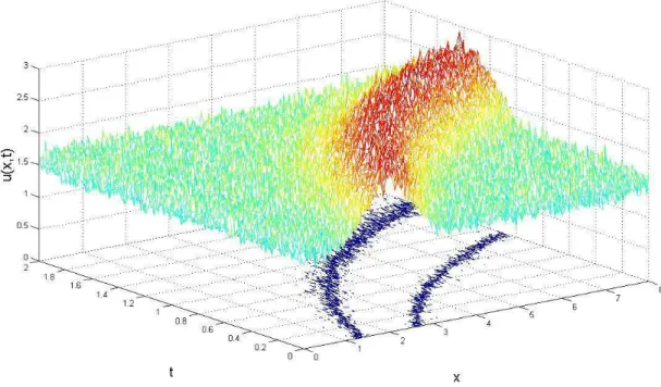
Figure 1 shows a simple example concerning the performance of the proposed methods when integrating the equation (1) on [0 2]×[0 8] with b = x, σ(t) = 2, and initial condition
u0(x) =e−2(x−2)
2
Figura 1: Computational integration of equation (1) by the proposed method.
4
Conclusions
In this work we introduce an effective numerical integrator for the computer simulation of the semi-linear stochastic transport equation (1). For this we develop a computational method which is obtained via the solution of an suitable caratheodory-like RDE resulting for a associated RIE together with the numerical integration of SDEs and RDEs. It is important to note that thanks to the particular structure of the involved matrix in the proposed method, the computational burden is considerably reduced -from dimension 2d+ 2 to dimension d- (via an adapted Pad´e method with scaling-squaring strategy) to the same computational load of solving simultaneous linear systems through a LU decomposition of a unique matrix. It is worth to note that the proposed method is well suited for parallel computing and since the computational cost scales with the dimension of the underlined original equation the approach has great potential even for very large simulation models.
5
Acknowledgement
FGV/EMAp project: ”Toolbox for the simulation and estimation of SDEs”
Referˆ
encias
[1] F. Carbonell, J.C. Jimenez, R.J. Biscay, H. de la Cruz, The Local Linearization method for numerical integration of random differential equations, BIT, 45 (2005) 1-14.
[2] F. Carbonell et al. The Local linearization method for the numerical integration of random differential equations. BIT, 45 (2005) p. 1-14.
[4] F. Dorini, M. C. Cunha, A finite volumen method for the mean of the solution of the random transport equation, Appl. Math. Comput 187 (2) (2007), 912-921.
[5] F. Dorini, M. C. Cunha, Statistical moments of the random linear transport equation, J. Comput. Phys 227 (2008), 8541-8550
[6] F. Flandoli, M. Gubinelli, E. Priola, 2010. Well-posedness of the transport equation by stochastic perturbation, Invent. Math., 180(1): 1-53
[7] Golub, G. H. and Van Loan, C. F. Matrix Computations. The Johns Hopkins University Press, 3th Edition, 1996.
[8] L. Grune, P. Kloeden, Pathwise approximation of Random Differential Equations. BIT, 41 (2001) p. 711-721.
[9] H. Kunita, First Order Stochastic Partial Differential Equations , Proceedings of the Tani-guchi International Symposium on Stochastic Analysis, 1984.
[10] H. Kunita, Stochastic flows and stochastic differential equations. Cambridge University Press. 1990
[11] C. Moler, C.F. Van Loan, Nineteen dubious ways to compute the exponential of a matrix, twenty-five years later, SIAM Review. 45 (2003) 3-49.
![Figure 1 shows a simple example concerning the performance of the proposed methods when integrating the equation (1) on [0 2] × [0 8] with b = x, σ(t) = 2, and initial condition u 0 (x) = e − 2(x−2)](https://thumb-eu.123doks.com/thumbv2/123dok_br/15687888.117636/5.918.305.606.79.163/figure-example-concerning-performance-proposed-integrating-equation-condition.webp)