Abstract
The components of flexible rotors are subjected to un-certainties. The main sources of uncertainties include the variation of mechanical properties. This contribu-tion aims at analyzing the dynamics of flexible rotors under uncertain parameters modeled as fuzzy and fuzzy random variables. The uncertainty analysis encom-passes the modeling of uncertain parameters and the numerical simulation of the corresponding flexible rotor model by using an approach based on fuzzy dynamic analysis. The numerical simulation is accomplished by mapping the fuzzy parameters of the deterministic flex-ible rotor model. Thereby, the flexflex-ible rotor is modeled by using both the Fuzzy Finite Element Method and the Fuzzy Stochastic Finite Element Method. Numeri-cal simulations illustrate the methodology conveyed in terms of orbits and frequency response functions sub-ject to uncertain parameters.
Keywords
Roto dynamics; uncertainty analysis; Fuzzy-random analysis.
Uncertainty analysis of flexible rotors considering fuzzy
parameters and fuzzy-random parameters
1 INTRODUCTION
Nowadays, the industrial applications require mechanical systems working with optimal performance subject to specific operational conditions, which demands: high reliability, robustness against envi-ronmental conditions and low operating requirements. Consequently, it is necessary to develop reliable numerical models that take into account uncertain parameters, and allow the prediction of the dy-namic behavior of the system under realistic conditions.
Fabian Andres Lara-Molinaa Edson Hideki Koroishib Valder Steffen Jrc
a,bFederal Technological University of Paraná
(UTFPR), Campus Cornélio Procópio, Av. Alberto Carazzai, 1640, Cornélio Procópio, PR, Brazil, ZIP CODE 86300-000
cFederal University of Uberlândia (UFU), School of
Mechanical Engineering, Campus Santa Mônica, Av. João Naves de Ávila 2121, Bloco 1M, Uberlândia, MG, Brazil, ZIP CODE 38400-902
Corresponding author:
a[email protected] b[email protected]
http://dx.doi.org/10.1590/1679-78251466
The components of flexible rotors are realistically subjected to uncertainties. The main sources of uncertainties include the variation of mechanical properties, such as damping, stiffness, and geomet-rical imperfections (Lalanne and Ferraris, 1998). The dynamic behavior of rotors is then affected by the uncertain parameters of the system. Consequently, the quantification of parametric uncertainties is necessary to predict how the dynamic response varies, by means of numerical models of industrial applications and research testbeds (Chowdhury and Adhikari, 2012). Ritto et al. (2011) considered parametric uncertainties to develop a methodology to optimize the performance of the flexible rotor and, so, they demonstrated that parametric uncertainties in the dynamic model represent a complex problem of engineering design. As mentioned above, the components of flexible rotors that are typi-cally subjected to uncertainty are the stiffness of the shaft (Young's Modulus), bearings (stiffness and damping coefficients) together with the dimensional tolerances of shafts and disks. Therefore, uncer-tain parameters should be taken into account in the numerical model in order to obuncer-tain reliable predictions in the computational simulations.
Uncertainty analysis of flexible rotors has been studied by applying stochastic approaches based on the Stochastic Finite Elements Method (Ghanem and Spanos, 1991). Didier et al. (2012) quantified the uncertainty effects in the response of flexible rotors based on the Polynomial Chaos Theory. Koroishi et al. (2012) represented the uncertainties in the rotor parameters by using Gaussian homo-geneous stochastic fields discretized by Karhunen-Loève expansion; the dynamic response of the sys-tem with uncertainties was characterized through Latin Hypercube Sampling and Monte Carlo Sim-ulation.
The fuzzy theory permits to model the uncertainty as an alternative to the stochastic methods. By means of fuzzy theory it is possible to describe incomplete and inaccurate information. The fuzzy sets theory was initially formulated by Zadeh (1965) to characterize the vague aspect of the infor-mation. Thereafter, Zadeh developed the theory of possibility based on fuzzy sets that can be com-pared to the theory of possibilities to deal with the uncertainty of information (Zadeh, 1978). The theory of fuzzy sets and the theory of possibilities are connected, so that it is possible to get along with the uncertainty and imprecision of the information sets by applying the fuzzy sets theory. Then, the uncertainties are modeled by means of fuzzy sets theory for the cases in which the stochastic process that describes the random variables is unknown. In this context, Moens and Hanss (2011) presented a literature review of the non-probabilistic approaches for the analysis of parametric uncer-tainty; they applied these methods to analyze structures modeled by the finite element method with uncertain parameters. The two principal approaches presented in this contribution to model the un-certainties are the interval analysis and the fuzzy approach. These two procedures require solving interval problems to compute the uncertain structural response. Several research works in this area attempt to implement alternative methods to simulate mechanical systems with fuzzy uncertain pa-rameters (Lara-Molina et al., 2014b; Waltz and Hanss, 2013; Farkas et al., 2008; Klimke, 2006). Specifically, Lara-Molina et al. (2014a) represented the uncertainties in the rotor parameters by using fuzzy variables and performing a fuzzy dynamic analysis.
In agreement with the fuzzy approach, the present work proposes the application of a straightfor-ward method to simulate the dynamic response of flexible rotors with uncertain parameters by per-forming a fuzzy dynamic analysis. For this purpose, the fuzzy uncertain parameters are mapped onto the model with the aid of α-level optimization Möller and Beer (2004).
The remainder of this paper has five sections. In section 2, the flexible rotor model based on the finite element method is shown. Section 3 presents the methodology to analyze the response of struc-tures with fuzzy parameters and fuzzy random parameters by using the Fuzzy Finite Element Method
and Fuzzy Stochastic Finite Element Method, respectively. Section 4 presents the numerical simula-tions of flexible rotor model in which the time and frequency responses were characterized by fuzzy and fuzzy random functions. Finally, the conclusions and the proposals of future work are outlined.
2 MODELING OF FLEXIBLE ROTORS
2.1 Theoretical background on the deterministic finite element modeling of a rotor system
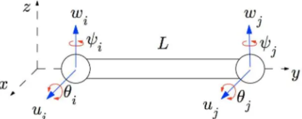
The dynamic response of the considered mechanical system can be represented by using principles of variational mechanics, namely the Hamilton`s principle. For this aim, the strain energy of the shaft and the kinetic energies of the shaft and discs are calculated. An extension of Hamilton`s principle makes possible to include the effect of energy dissipation. The parameters of the bearings are included in the model by using the principle of the virtual work. For computational purposes, the finite element method is used to discretize the structure so that the energies calculated are concentrated at the nodal points. Shape functions are used to connect the nodal points (Morais et al., 2010). In this model, 4 degrees of freedom per node are taken into account, namely two displacements (u and w) and the
cross-section rotations about axes x and z (denoted by w y and u y, respectively). Fig. 1 shows the finite element used to model the rotor.
Figure 1: Illustration of the shaft finite element (Simões et al., 2007).
According to Lalanne and Ferraris (1998) the model depicted in Fig. 1 can be represented mathemat-ically by the following set of differential equations:
( )t ( S ) ( )t ( )t ( )t
Mq C G q Kq F (1)
where ( ) N N
S D R
M M M and ( ) N N
S B R
K K K are, respectively, the mass and
stiff-ness matrices, C(CB CP)RN N is the damping matrix formed by the contributions of the
viscous damping matrix, CB, and the inherent proportional damping matrix, CP MMKK and
( ) N N
S D R
G G G designates the gyroscopic matrix formed by the gyroscopic contributions of
the rigid discs and the shaft. q( )t RN and F( )t RN are, respectively, the vectors of the amplitudes
of the harmonic generalized displacements and external loads, S is the angular speed of the shaft, and M and K represent, respectively, the proportional coefficients of mass and stiffness.
Lima et al. (2010) used the receptance or Frequency Response Function (FRF) matrix to analyze the deterministic system, whose components are complex functions of the excitation frequency that establish linear relations between the amplitudes of the harmonic responses and the amplitudes of the excitation forces and moments, as expressed by Eq. (2):
1
1 2
ˆ
( , S) ( , S) ( ) i( s ) ( )
Q H F M C G K F (2)
where ( , ) N
S R
Q and F( ) RN are, respectively, the vectors of the amplitudes of the harmonic
generalized displacements and external loads.
2.2 Parameterization of the deterministic FE model
At this point it is important to consider that, in order to study the system behavior when uncertainties are to be taken into account, the uncertain responses have to be computed with respect to a set of uncertain geometrical and/or physical parameters associated with the flexible rotor. In general, such uncertain variables intervene in a rather complicated manner in the finite element matrices. Hence, for evaluating the variability of the responses associated with these uncertainties, it becomes inter-esting to perform a parameterization of the FE model, which is understood as a means of making the design parameters factored-out of the elementary matrices. At the expense of lengthy algebraic ma-nipulations, this procedure makes it possible to introduce not only the uncertainties into the flexible rotor model, but also to perform a sensitivity analysis in a straightforward way, leading to significant cost savings in iterative robust optimization and/or model updating processes. After manipulations, those parameters of interest can be factored-out of the elementary matrices as indicated below:
Shaft
=
( ) ( )
( ) ( )
( ) ( )
e e
S S S SS
e e
S S S S
e e
S S S S A E I I M M K K G G (3)
Bearing
=
( ) ( ) ( )
( ) ( ) ( )
e e e
B xx B zz B
e e e
B xx B zz B
k k d d
K K K
C C C
(4)
where S, AS, IS and ES represent, respectively, the mass density, the cross-section area, the inertia
and the Young’s modulus of the shaft. dxx , dzz and kxx, kzz designate, respectively, the damping and
stiffness coefficients of the bearings. It is worth mentioning that the matrices appearing in the right hand side of Eqs. (3) and (4) are those from which the design parameters of interest have been factored-out.
3 FUZZY AND FUZZY STOCHASTIC ANALYSIS
In several cases, some parameters of the systems cannot be accurately estimated due to small varia-tions around its nominal value. In these cases, these parameters can be modeled by means of fuzzy variables. As mentioned above, the fuzzy set theory was initially formulated by Zadeh (1965) to
represent vague or ambiguous information. Thereby, it is possible to represent inaccurate or uncertain parameters by using fuzzy variables, especially when the stochastic process which models the uncer-tain parameter cannot be determined by a simple observation.
In this section a brief introduction to two different numerical methods is presented, with the purpose of quantifying the uncertain structural response. First, the fuzzy analysis computes the un-certain structural response when the unun-certain parameters are modeled as fuzzy variables that repre-sent the uncertain parameters. The methodology to analyze the fuzzy uncertainties is based on level optimization, previously presented by Möller et al. (2000); thus, an optimization problem is solved to obtain the fuzzy output of the system by means of level optimization.
In the other hand, the fuzzy stochastic analysis computes the uncertain structural response of the system when the parameters are modeled such as fuzzy-random variables (Möller et al., 2009). These types of variables quantify uncertainties produced by variable and random sources. The fuzzy sto-chastic analysis algorithm encompasses a fuzzy analysis and a stosto-chastic analysis to cope with the fuzziness and randomness characteristics of the uncertainties. It is worth mentioning that both afore-mentioned analyses are relying on the deterministic model of the system.
3.1 Fuzzy Variables
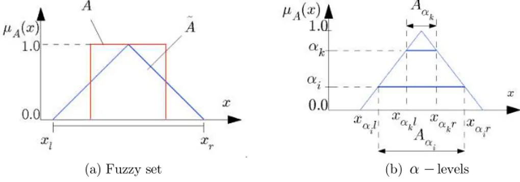
Let X be an universal set of objects whose generic elements are denoted by x. The subset A (where, A X) is defined by the classical membership function A :X
0,1 (see Fig. 2(a)). Furthermore,a fuzzy set A is defined by means of the membership function A :X 0,1, where 0,1 is a
continuous interval. The membership function indicates the degree of compatibility of the element x
to A. The closer the value of A( )x to “1”, the more x belongs to A.
(a) Fuzzy set (b) levels
Figure 2: Fuzzy set and level representation.
For numerical purposes, Möller and Beer (2004) represented the fuzzy variables as intervals weighted by a membership function using the level representation. Thus, the fuzzy set is completely defined by:
, A( )
, where 0 A 1A x x x X (5)
For computational purposes, the fuzzy set A can be represented by means of subsets that are
de-nominated levels. These subsets, which correspond to real and continuous intervals, are defined by
K
A (see Fig. 2(b)), thus:
, ( )
K A K
A x X x (6)
The level subsets of A have the property:
, (0,1] whit
K i i K i k
A A (7)
If the fuzzy set is convex (in the unidimensional case), each level subset K
A corresponds to
the interval xkl,xkr where:
min , ( )
max , ( )
K
K
l A K
r A K
x x x
x x x
X X (8)
3.2 Fuzzy Random Variables
The fuzzy random variables were defined previously by (Kwakernaak, 1978; Puri and Ralescu, 1986). According to the probability theory, the space of random elementary events is presented. A fuzzy realization of the form x
xX is assigned to each elementary event . Accordingly, afuzzy random variable X is the fuzzy result of the uncertain mapping
: ( )
X F X (9)
where F X( ) is the set of all fuzzy numbers on n. Each real random variable X on X is contained
in X.
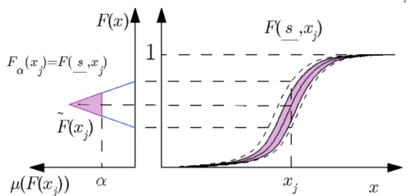
Based on this definition, a fuzzy random variable X can be described by a fuzzy cumulative
distribution function F
x . Considering an original value xj, the fuzzy probability distributionfunction F
xj can be represented as the set of probability distribution functions with membershipvalue
F x
j
(see Fig. 3). F
xj is associated to the fuzzy bunch parameter s in order to parameterize the fuzziness of F
x (Möller and Beer 2005), thus:
,
F x F s x (10)
Thereby, for numerical computation, the discretization is properly used.
,
( ), ( ( ))
( ) min, ( ); max, ( ) ;
( )
(0,1]
F s x F x F x F x F x F x F x (11)
with
min,
max,
( ) min ( , )
( ) max ( , )
F x F s x s S
F x F s x s S
Figure 3: discretization of F s x
,
, adapted from (Möller and Beer, 2004).For example, the fuzzy bunch parameters s1 and s2 can be used to represent the fuzzy mean and
fuzzy standard deviation of a fuzzy normal probability distribution as in eq. (12)
12
1
, 1
2 2
x s
F s x erf
s
(12)
3.3 Dynamic Models with Fuzzy Parameters
In the context of this work, the model describes the dynamic behavior of the rotor by means of a set of differential equations. The relationship between the inputs x and outputs z of an specific dynamic
model M is characterized by f , which represents the set of differential equations of the model in the
Eq. (13).
: ( ) ( )
M z f x (13)
Therefore, the function f maps the inputs x onto the outputs z( ) , thus x z( ) , where is
the independent variable of the dynamic response that may represent time, frequency or spacial coordinates.
When considering the inputs of the model as fuzzy variables x or fuzzy functions x
, thedynamic response of the system corresponds to the resulting fuzzy functions z
. These fuzzyfunc-tions result of the mapping, thus xz
.3.4 Fuzzy Dynamic Analysis
The fuzzy dynamic analysis is an appropriate method to map a fuzzy input vector x onto the fuzzy
output z
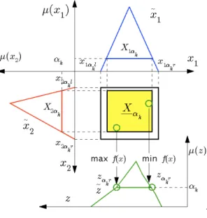
of a numerical model using the deterministic model given by Eq. (13). In structuralanalysis, the combination of uncertainties modeled as fuzzy variables with the deterministic model based on Finite Element Method is denominated Fuzzy Finite Element Method. The fuzzy dynamic analysis is composed of two stages shown in Fig. 4.
In the first stage, for computational purposes, the input vector that corresponds to the fuzzy parameter is discretized by means of level representation, presented in Eq. (6) and Fig. 2(b).
Thus each element of the fuzzy parameters vector x
x1,...,xn
is considered as an interval ,k k
k
i i l i r
X x x , where k (0,1]. Consequently, the sub-space Xk is defined so that
k
X
X1k,,Xnk
, where kn X .
The second stage is related to solving an optimization problem. This optimization problem consists in finding the maximum and minimum value of the output, at each evaluated value , for the mapping model M :z f x( ), thus:
max ( ) min ( )
K K
K K
r l
x X x X
z f x z f x
(14)
kr
z and
kl
z correspond to the upper and lower bounds of the interval ,
k kr kl
z z z in the
level k. The set of discretized intervals ,
kr kl
z z
for k (0,1] composes the whole fuzzy resulting
variable z.
Figure 4: Level optimization.
The fuzzy analysis of a transient time-domain system demands the solution of a large number of optimization problems regarding all level of interest for each considered time step. Each upper and lower bounds of the system analysis at a given time instant is obtained by using the Differential Evolution optimization algorithm (Price et al., 2005). The output value of the transient analysis at the evaluated time-step constitutes the objective function. The inputs to this function are the uncer-tain parameters described previously as fuzzy or fuzzy random variables.
3.5 Fuzzy Stochastic Analysis
In structural analysis, the combination of uncertainties modeled by using fuzzy randomness with the deterministic model based on Finite Element Method is denominated Fuzzy Stochastic Finite Element Method.
Fuzzy stochastic analysis is a straightforward computational method for processing uncertain data modeled by fuzzy random functions or variables. The aim of fuzzy stochastic analysis is to map fuzzy random parameters X onto the structural fuzzy random response Z
, thereby, the followingprob-lem is to be solved for a crisp mapping model
X Z (15)
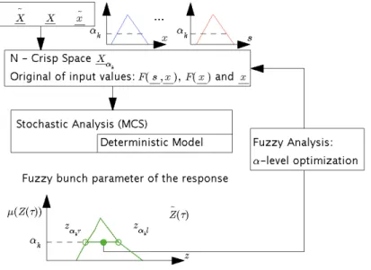
The diagram of Fig. 5 shows the fuzzy stochastic analysis algorithm. The basic concepts and definitions of the fuzzy stochastic analysis are presented with more details by Möller and Beer (2004).
Figure 5: Fuzzy stochastic analysis, adapted from (Möller and Beer 2004).
The uncertainty model determines the type of the uncertain parameters. In this method an uncertain parameter can be modeled as a real random variable, fuzzy variable or fuzzy randomvariable and/or functions; e.g. a normally distributed fuzzy random variable with fuzzy mean and fuzzy standard deviation. Fuzzy variables and/or real random variables are special cases of fuzzy random variables. Moreover, the Karhunen Loève expansion can be used to represent a real random field.
The fuzzy random parameters are modeled as fuzzy random variables, which represent a general-ized model i.e., high order uncertainty representation. The fuzziness of the fuzzy random variables X
is described by means of fuzzy bunch parameters. Thereby, the fuzzy bunch parameters s of Eq. (10)
are discretized by using the level representation; thus, the level sets of Eq. (6) are obtained for the corresponding intervals of each determined level.
The fuzzy stochastic analysis algorithm encompasses a fuzzy analysis and a stochastic analysis to deal effectively with the fuzziness and randomness characteristics of the uncertainties (see Fig. 5). Both analyses are based on the deterministic model.
The purpose of fuzzy analysis is to map fuzzy input variables and fuzzy bunch parameters of the fuzzy random variables onto fuzzy random response; thus, the resulting fuzzy bunch parameters of the fuzzy random response are obtained. The level optimization as stated by Möller et al. (2000)
is applied in the fuzzy analysis. An extended formulation of the fuzzy analysis based on the � -opti-mization was previously presented in Sec. 3.4.
In the stochastic analysis each element of fuzzy set s determines an original real random variable of every fuzzy random variable and an original deterministic value of every fuzzy variable. These original variables are mapped onto the original function Z( ) of fuzzy random result values Z
by a stochastic analysis. The mapping model is to be established by a stochastic analysis and it is based on the Finite Element approach, thus leading to the Stochastic Finite Element Method. Ac-cordingly, the Monte Carlo Simulation is an appropriated method to perform the stochastic analysis. The result of a Monte Carlo sampling is an original function Z( ) of the fuzzy random response
Z at the membership level
Z
k. The optimization problem of the �-leveloptimi-zation is solved so that the assigned elements ,
k kr kl
z z z at the specific membership level k
(e.g. fuzzy mean or fuzzy variance) of the fuzzy random results are found.
4 NUMERICAL SIMULATIONS
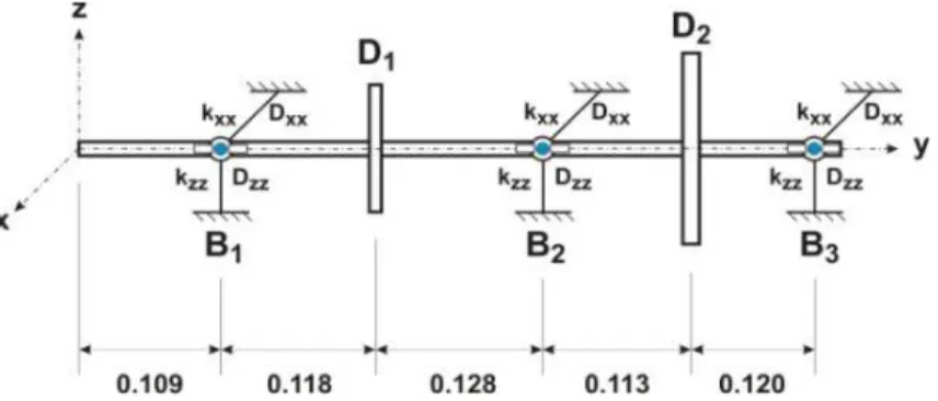
The proposed methodology was numerically applied to analyze the dynamic behavior of a rotor system composed of a horizontal flexible steel shaft, modeled by 20 Euler-Bernoulli's beam elements, two rigid steel discs (D1 and D2) and three asymmetric bearings (see Fig. 6).
Figure 6: Flexible rotor (Cavalini Jr et al., 2011).
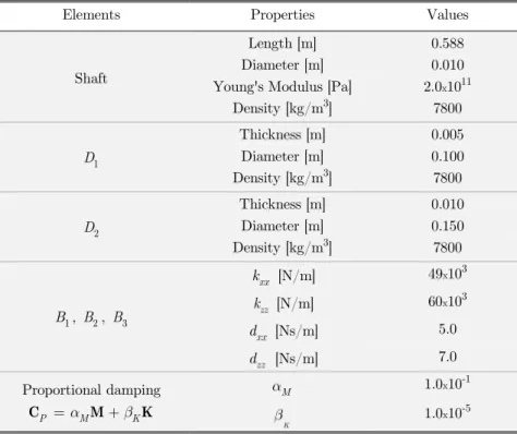
The physic and geometric properties of the shaft, discs and bearings are given in Table 1. The matrix equation of motion of the studied rotor was solved by using a MATLAB/SIMULINK® code. In all analyses performed in this contribution, the model considered only the first six vibration modes of the rotor, measured along the x and z directions at the positions of the bearings.
The parameters used in the Differential Evolution Algorithm to solve the optimization problem in the fuzzy analysis are described as follows: population size is 10 per uncertain variable, 100 genera-tions, crossover probability rate is 0.8, perturbation rate is 0.8 and the strategy for the mutation mechanism is DE/rand/1/bin. These parameters were derived from previous contributions (Price et al., 2005). The two objective functions for the optimization problem are the following: the norm
ˆ( ,S)
H and the generalized displacements q( )t to compute both the FRF and the orbits; the
corresponding expressions are given by Eq. (2) and (1). The uncertain parameters were considered by means of fuzzy triangular numbers, which is the simplest representation to describe a fuzzy variable.
Elements Properties Values
Shaft
Length [m] 0.588
Diameter [m] 0.010
Young's Modulus [Pa] 2.0x10¹¹
Density [kg/m3] 7800
1
D
Thickness [m] 0.005
Diameter [m] 0.100
Density [kg/m3] 7800
2
D
Thickness [m] 0.010
Diameter [m] 0.150
Density [kg/m3] 7800
1
B , B2, B3
xx
k [N/m] 49x103
zz
k [N/m] 60x103
xx
d [Ns/m] 5.0
zz
d [Ns/m] 7.0
Proportional damping
P M K
C M K
M
1.0x10⁻¹
K
1.0x10⁻⁵
Table 1: Physic and geometric properties of the rotor elements.
Two case studies are considered to analyze the uncertain dynamic behavior of the flexible rotor. In the first case, the uncertain parameters are modeled as fuzzy variables to perform the fuzzy modeling. In the second case, the uncertain parameters are modeled as fuzzy random variables, thus the fuzzy stochastic modeling is performed.
4.1 Fuzzy Analysis
In this contribution, the uncertainties are considered in the Young's Modulus ES of the shaft and in
the parameters (stiffness and damping) of the bearings (B1, B2 and B3). The uncertain parameters
are modeled by using fuzzy triangular numbers, thus: aa
1p/ 100 / 1 / 1p/ 100
where a represents the nominal value of the parameter and p stands for the maximum percentage ofamplitude in 0. To investigate the influence of uncertainties on the flexible rotor, three
uncer-tainty scenarios were considered. Table 2 presents the percentages of variation of the triangular fuzzy variables corresponding to the uncertainty scenarios that are taken into consideration in the numerical simulations.
Scenarios Shaft Bearings
S
E kxx kzz dxx kzz
(a) 15% ─ ─ ─ ─
(b) ─ 5% 5% 5% 5%
(c) 15% 5% 5% 5% 5%
Table 2: Uncertainty scenarios for fuzzy modeling.
The first scenario was dedicated to investigate the influence of uncertainties only in the shaft (Young's Modulus ES). The second one took into account only uncertainties in the bearings. Finally, the third
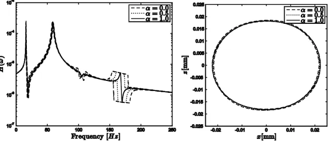
scenario has considered uncertainties both in the shaft and the bearings. In these three uncertain scenarios, the Frequency Response Functions (FRFs) along both the directions x and z and the orbits of rotor were analyzed. Fig. 7 shows the Frequency Response Function (FRF). The fuzzy structural response of the rotor was computed for three different values where 1.0, 0.5,
0.0
.
The variation of the Young's Modulus ES of the shaft produced a variation in the third natural
frequency and also small changes in the amplitude of the first two natural frequencies.
For observing the system's behavior in the time domain, the orbit of the disc 1 is shown in Fig. 8. For the three uncertain scenarios, the rotor is operated at 600 rpm. The choice of this rotation speed is justified by considering that this rotation is well above the first two natural frequencies, so that it is guaranteed that the rotor will not operate in the proximity of a critical speed for any fuzzy model. Figure 8 shows that the uncertainties influence the amplitude of displacement; this influence can be observed in the small variation of the lower and upper envelopes of the orbits.
Figure 7: FRFs, case (a). Figure 8: Envelope of the orbits, case (a).
For the scenario (b), the uncertainties are introduced only in the parameters of the bearing, namely the stiffness and damping. The FRFs and orbits are shown, respectively, in Figs. 9 and 10. The FRFs (see Fig. 9) shows that the uncertainties of the bearings result in a small variation of the amplitude at the two natural frequencies. The main difference between the FRFs of scenario (a) and the FRFs of scenario (b) occurs in the natural frequency near 165 Hz. For the scenario (b) there is a very small variation of the third natural frequency.
Analyzing the orbit shown in Fig. 10, for the second scenario, and comparing with the orbit shown in Fig. 8, it is possible to see that the uncertainty applied in the first scenario results in a smaller change in the orbits (see again the orbits shown in Fig. 8). However, the uncertainties in the stiffness and damping coefficients of the bearing result in important variations on the displacement of the rotor.
Figure 9: FRFs, case (b). Figure 10: Envelope of the orbits, case (b).
Finally, the scenario (c) considers the uncertainties in the shaft (Young's Modulus) and bearings (stiffness and damping coefficients), simultaneously. Figs. 11 and 12 show, respectively, the FRFs and the orbits. The results presented by the scenario (c) permit to observe the combined influence of the uncertainty parameters on the dynamic behavior of the system. The result of this combination of uncertainty parameters leads to an important variation between the lower and upper curves of the envelope.
Figure 11: FRFs, case (c). Figure 12: Envelope of the orbits, case (c).
In terms of FRFs, the influence of the uncertain ES is characterized by a variation at the third
natural frequency shown in Fig. 11, while the uncertainties in the bearings influence the amplitudes at the first two natural frequencies. Analogously, in terms of the orbits, a similar influence is observed.
In this scenario, the uncertainties in the stiffness of the shaft and damping coefficients of the bearings produce a combined effect in the envelop of the orbit, as illustrated in Fig. 12.
4.2 Fuzzy Stochastic Analysis
The fuzzy stochastic analysis of sec. 3.5 allows evaluating uncertain parameters modeled as fuzzy variables, real random variables and fuzzy random variables. Nevertheless, in order to demonstrate the performance of this method the parameters of the bearings are modeled as fuzzy-random vari-ables with a fuzzy mean. This analysis aims at determining the orbits of the flexible rotor when the stiffness and viscous damping of the bearings are modeled as fuzzy random variables. Thereby, the fuzzy stochastic analysis method of sec. 3.5 is applied. The fuzzy random variables are defined to be normally distributed with a fuzzy mean m m
1p/ 100 / 1 / 1p/ 100
where p is themaximum percentage of the amplitude for the case in which 0 and m holds for the nominal
value of each parameter. Additionally, the uncertainty of the Young's Modulus of the shaft ES is
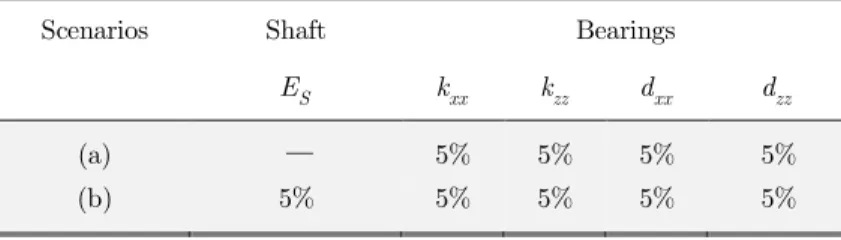
taken into account. Therefore, the stochastic model of the flexible rotor and specifically the stiffness of the shaft was modeled as a Gaussian random field by means of the Karhunen-Loève decomposition such as implemented by Koroishi et al. (2012). Therefore, two uncertain scenarios are analyzed as described in Table 3: in the first scenario, the influence of the bearings is analyzed; in the second uncertain scenario, the uncertainty introduced in the bearings and shaft is taken into account simul-taneously.
Scenarios Shaft Bearings
S
E kxx kzz dxx dzz
(a) ─ 5% 5% 5% 5%
(b) 5% 5% 5% 5% 5%
Table 3: Uncertainty scenarios for fuzzy stochastic modeling.
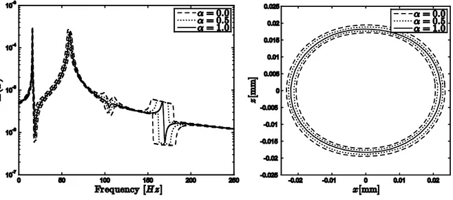
The results presented by the scenario (a) in Fig. 13 shows how fuzzy random damping and stiffness of the bearings affect the orbit of the shaft. The results show the fuzzy mean evaluated for 0.0
and 1.0. Additionally, the envelope of the uncertain orbit is bounded by the outer and the inner curves. The results show the influence in the amplitude of the displacements taking into account uncertainties that consider fuzziness and randomness characteristics. Consequently, the fuzzy random uncertainties introduced in the coefficients of the bearings produce a large variation in the envelopes of the orbit with respect to fuzzy modeling in which the uncertainties were considered only as fuzzy variables.
The results of the scenario (b) (see Fig. 14) show the combined influence of the uncertain fuzzy random coefficients of the bearings and the uncertain stiffness of the shaft. The fuzzy mean has not significant changed as compared with the previous uncertainty scenario. Nevertheless, the uncertain stiffness of the shaft produces a large variation in the inner curve of the envelope with respect to the previous uncertain scenario. As seen, this method allows evaluating simultaneously uncertain param-eters of the rotor modeled as fuzzy random variables and Gaussian random fields.
Figure 13: Envelope of the orbits, case (a). Figure 14: Envelope of the orbits, case (b).
5 CONCLUSIONS
In this contribution the uncertainty analysis of a flexible rotor by using Fuzzy Finite Element Method
and Fuzzy Stochastic Finite Element Method was proposed and implemented. The uncertainties in the parameters that characterize the rotor system are introduced directly through a parametric ap-proach and modeled as fuzzy variables and fuzzy random variables. The orbits and frequency response functions of the flexible rotor with uncertain parameters are simulated by using fuzzy stochastic dynamic analysis method. The numerical results indicate the degree of influence of the fuzzy uncertain variables on the dynamic behavior of the rotor. The strategy used in this work demonstrated to be straightforward for design and analysis of rotating systems. The selection of the uncertain fuzzy variables (stiffness, modulus of elasticity) was based on a previous knowledge regarding their sensi-tivities with respect to the frequency response functions. It is worth mentioning that these parameters are directly associated with the dynamic behavior of the rotor as represented by the orbits for the various uncertain scenarios considered. Additionally, the results show that the performance of the rotor, in terms of orbits and frequency response functions, are similar to the stochastic approach accomplished by Koroishi et al. (2012) in previous studies.
The uncertain parameters were properly described as fuzzy variables and fuzzy random variables. Fuzzy variables are a simple representation of uncertainties in which it is not necessary to know the probability distribution function of the stochastic variables. Fuzzy random variables permit to model high order uncertainties, which characterize fuzziness and randomness aspects of the uncertainty. However, the main disadvantage of the fuzzy analysis and fuzzy stochastic analysis is the necessity of solving the α-level optimization problem, which often demands high computational effort.
Further work will include an experimental verification aiming at evaluating the effect of variable parameters modeled as fuzzy variables on the dynamic behavior of rotating machines.
Acknowledgements
The authors express their acknowledgements to the National Institute of Science and Technology of Smart Structures in Engineering (INCT-EIE), jointly funded by CNPq, CAPES and FAPEMIG.
References
Cavalini Jr., A.A., Galavotti, T.V., Morais, T.S., Koroishi, E.H., Steffen Jr, V., (2011). Vibration attenuation in rotating machines using smart spring mechanism. Mathematical Problems in Engineering 2011(340235), 14.
Chowdhury, R., Adhikari, S., (2012). Fuzzy parametric uncertainty analysis of linear dynamical systems: A surrogate modeling approach. Mechanical Systems and Signal Processing 32: 5-17.
Didier, J., Faverjon, B., Sinou, J.J., (2012). Analyzing the dynamic response of a rotor system under uncertain param-eters by polynomial chaos expansion. Journal of Vibration and Control 18(5): 587-607.
Farkas, L., Moens, D., Vandepitte, D., Desmet, W., (2008). Application of fuzzy numerical techniques for product performance analysis in the conceptual and preliminary design stage. Computers and Structures 86: 1061-79.
Ghanem, R.G., Spanos, P.D., (1991). Stochastic finite elements: A spectral approach. Courier Dover Publications. Klimke, W.A., (2006). Uncertainty modeling using fuzzy arithmetic and sparse grids. PhD thesis, Universität Stuttgart. Koroishi, E.H., Cavalini, A.A.J., de Lima, A.M.G., Steffen Jr, V., (2012). Stochastic modeling of flexible rotors. Journal of the Brazilian Society of Mechanical Sciences and Engineering 34 (Special Issue): 597-603.
Kwakernaak, H., (1978). Fuzzy random variables - I. Definitions and theorems. Information Sciences 15(1): 1-29. Lalanne, M., Ferraris, G., (1998). Rotordynamics - Prediction in Engineering. John Wiley & Sons, New York. Lara-Molina, F.A., Koroishi, E.H., Steffen Jr, V., (2014a). Fuzzy stochastic dynamic analysis of flexible rotors. Pro-ceedings of the 2nd International Symposium on Uncertainty Quantification and Stochastic Modeling.
Lara-Molina, F.A., Koroishi, E.H., Steffen Jr, V., (2014b). Técnicas de inteligência computacional com aplicações em problemas inversos de engenharia. Chapter Análise estrutural considerando incertezas paramétricas fuzzy. Omnipax Editora.
Lima, A.M.G., Faria, A.W., Rade, D.A., (2010). Sensitivity analysis of frequency response functions of composite sandwich plates containing viscoelastic layers. Composite Structures 92(2): 364-76.
Moens, D., Hanss, M., (2011). Non-probabilistic finite element analysis for parametric uncertainty treatment in applied mechanics: Recent advances. Finite Elementsin Analysis and Design 47(1).
Möller, B., Beer, M., (2004). Fuzzy Randomness, Uncertainty in Civil Engineering and Computational Mechanics. Springer-Verlag.
Möller, B., Graf, W., Beer, M., (2000). Fuzzy structural analysis using α-level optimization. Computational Mechanics 26: 547-65.
Möller, B., Beer, M., (2004). Fuzzy randomness, Uncertainty in civil engineering and computational mechanics. Springer-Verlag.
Möller, B., Graf, W., Sickert, J.-U. Steinigen, F., (2009). Fuzzy random processes and their application to dynamic analysis of structures. Mathematical and Computer Modelling of Dynamical Systems: Methods, Tools and Applications in Engineering and Related Sciences 15(6): 515-34.
Morais, T.S., Steffen Jr, V., Mahfoud, J. (2010). Control of the breathing mechanism of a cracked rotor by using electro-magnetic actuator: numerical study. Latin American Journal of Solids and Structures 9(5): 581-596.
Price, K.V., Storn, R.M., Lampinen, J.A., (2005). Differential evolution a practical approach to global optimization. Springer-Verlag.
Puri, M.L., Ralescu, D.A., (1986). Fuzzy random variables. Journal of Mathematical Analysis and Applications 114(2): 409-22.
Ritto, T.G., Lopez, R.H., Sampaio, R., de Cursi, J.E.S., (2011). Robust optimization of a flexible rotor-bearing system using the campbell diagram. Engineering Optimization 43(1): 77-97.
Simões, R.C., Steffen Jr, V., Der Hagopian, J., Mahfoud, J., (2007). Modal active control of a rotor using piezoelectric stack actuators. Journal of Vibration and Control 13: 45-64.
Waltz, N.-P., Hanss, M., (2013). Fuzzy arithmetical analysis of multibody systems with uncertainties. The archive of mechanical engineering LX(1): 109-125.
Zadeh, L., (1965). Fuzzy sets. Information and Control 8: 338-53.
Zadeh, L., (1978). Fuzzy sets as basis for a theory of possibility. Fuzzy Sets and Systems 1: 3-28.