Differential Equations
H. de la Cruz,[email protected]1J.C. Jimenez,[email protected]2
1Fundac˜ao Get´ulio Vargas - Escola de Matem´atica Aplicada. Praia de Botafogo 190. Botafogo. Rio de Janeiro
2Instituto de Cibern´etica, Matem´atica y F´ısica - ICIMAF. Calle 15 No. 551, Vedado, C. Habana
Abstract. Over the last few years there has been a growing and renovated interest in the numerical study of Random Differential Equations (RDEs). On one hand it is motivated by the fact that RDEs have played an important role in the modeling of physical, biological, neurological and engineering phenomena, and on the other hand motivated by the usefulness of RDEs for the numerical analysis of Ito-stochastic differential equations (SDEs) -via the extant conjugacy property between RDEs and SDEs-, which allows to study stronger pathwise properties of SDEs driven by different kind of noises others than the Brownian. Since in most common cases no explicit solution of the equations is known, the construction of computational methods for the treatment and simulation of RDEs has become an important need. In this direction the Local Linearization (LL) approach is a successful technique that has been applied for defining numerical integrators for RDEs. However, a major drawback of the obtained methods is its relative low order of convergence; in fact it is only twice the order of the moduli of continuity of the driven stochastic process. The present work overcomes this limitation by introducing a new, exponential-based, high order and stable numerical integrator for RDEs. For this, a suitable approximation of the stochastic processes present in the random equation, together with the local linearization technique and an adapted Pad´e method with scaling and squaring strategy are conveniently combined. In this way a higher order of convergence can be achieved (independent of the moduli of continuity of the stochastic processes) while retaining the dynamical and numerical stability properties of the low order LL methods. Results on the convergence and stability of the suggested method and details on its efficient implementation are discussed. The performance of the introduced method is illustrated through computer simulations.
Palavras-chave: random differential equations, numerical integrators, exponential methods, Local linearization methods
1. INTRODUCTION
In several physical, chemical, industrial and biological phenomena, noise plays a significant role. This is the case, for example, in turbulent diffusion, epidemiology, genetic regulation, chemical kinetic, biological waste treatment, polymer dynamics, large scale integrated (VLSI) circuit design, finance, neurosciences, to mention just a few. When the evolution of such noisy phenomena has to be studied stochastic effects need to be taken into account, thus the mathematical modeling of such situations is not well matched by deterministic differential equations. There are, of course, many ways to introduce randomness into a mathematical models. In particular, during the last decades, in order to construct more realistic models, Random Differential Equations (RDEs) of the form
x′(t) =f(t,x(t), ξ(t)), t∈[t0, T],
(which are pathwise Ordinary Differential Equations (ODEs) containing a multidimensional stochastic processξin their vector field function), have been used in a wide range of applications, see e.g. [1], [12], [11], [10], [14], [15], [16]. Since, unfortunately, closed-form solutions of these equations are rarely available, the construction of computational methods for the treatment and simulation of RDEs has become an important need.
sample paths of the solutions are certainly continuously differentiable, but their derivatives are at most H¨older continuous in time. The resulting vector fieldf(t,x(t), ξ(t))is, thus, at most H¨older continuous in time, no matter how smooth the vector field is in its original variables. Consequently, since the usual estimates of the discretization error of such schemes require sufficient smoothness of the vector field function, numerical schemes for ODEs when applied to RDEs are not convergent or rarely attain their traditional order.
On the other hand, similar to the deterministic scenario, there exists a variety of important issues in designing practical numerical integrators for RDEs. In particular high accuracy, computational efficiency, and stability of the numerical schemes, are very desirable properties. Taking all this into consideration, some numerical integrator have been proposed in literature e.g., [2], [6], [8], [3]. However, these methods or are of implicit nature (involving the numerical solution of a system of nonlinear algebraic equations at each integration step, that typically increase the computational effort of these numerical integrators) or are explicit integrators, having the appealing feature of retaining the standard order of convergence of the classical deterministic schemes, but at the expense of high computational cost and low stability.
The aim of this paper is overcome these limitations by introducing a new, exponential-based, higher order, stable and explicit integrator for RDEs. For this, a suitable approximation of the stochastic processes present in the random equation, together with the local linearization technique and an adapted Pad´e method with scaling and squaring strategy are conveniently combined. In this way a higher order of convergence can be achieved (independent of the moduli of continuity of the stochastic processes) while retaining the dynamical and numerical stability properties of the low order LL methods proposed in [3] and with a suitable computational effort.
The paper is organized in 4 sections as follows. After this introduction, section2 presents the deduction of the proposed method, also a Pad´e algorithm is conveniently adapted and details on the effective implementation of the method is given. In section3the proposed method is evaluated by mean of simulations and finally in section4some concluding remarks are presented.
2. A HIGHER ORDER METHOD FOR RDES
Let(Ω,F, P)be a complete probability space, and(Ft)t≥0be an increasing right continuous family of complete sub σ-algebras ofF. Consider thed-dimensional random integral equation (see [7])
x′(t) =f(t,x(t), ξ(t)), t∈[t0, T], (1)
x(t0) =x0,
whereξtis aFt-adapted finite continuous processes.
2.1. Formulation of the method
Let(t)h ={tn : n= 0,1, . . . , N}be a partition of the time interval[t0, T], with equidistant stepsizeh < 1, i.e., defined as a sequence of timest0< t1< . . . < tN =T such thattn =t0+nh,forn= 0,1, . . . , N.
Starting from the initial valuex0,the approximations{xi}to{x(ti)},(i= 1,2, . . . , N)are obtained recursively as
follows.
For each time intervalΛn = [tn, tn+1]we consider the random local problem
x(t) =xn+
Z t
tn
f(s,x(s), ξ(s))ds, (2)
Then, the idea is to get an approximation ofx(tn+1), through the solution of the auxiliary random equation resulting from approximatingf and the stochastic increment. For this, let´s consider¯h=hγ(we need to take¯hin this way in order
to guaranty the order of convergence of the method we are constructing here) withγ≥2and such thath1−γ ∈Nand let
(tn)¯h={tin:tin=tn+i¯h, i= 0,1, . . . ,
h1−γ+ 1}a partition ofΛ n.
Fort∈Λn, definent= max{k:tkn≤t < tnk+1}.Then by a linear interpolation toξ(t)in[tnnt, tnnt+1]
ξ(t)≈ξ¯(t) =ξ(tnt
n ) +
∆ξ(tnt
n )
¯
h (t−t
nt
n ), (3)
It follows, by using the approximations above and a first order Taylor expansion offat(tn,xn, ξn), that the solution
of (2) inΛncan be approximated by the solution of the (pathwise) differential equation
x(t) =xn+ t
R
tn
(f(tn,xn, ξn)+fx(tn,xn, ξn)(x(s)−xn) +ft(tn,xn, ξn)(s−tn) (4)
+ [h1−γ]
X
k=0
t
R
tn (f′
ξ(tn,xn, ξn)
(ξtk
n−ξn) + ∆ξ(tkn)
¯
h (s−t
k n)
1[tk
n t k+1
Let’s denote
An =fx(tn,xn, ξn)
bkn =ft(tn,xn, ξn) +f
′
ξ(tn,xn, ξn)
∆ξ(tk n)
¯
h
ckn =f(tn,xn, ξn)−Anxn−f
t(tn,xn, ξn)tn+f
′
ξ(tn,xn, ξn)((ξtk
n−ξn)− ∆ξ(tk
n)
¯
h )t
k n
Then, the solution of (4) att = tn+1 is obtained as follows. Starting at x(t0n) = x(tn) = xn,x(tkn+1)is computed
recursively fromx(tk
n)by solving in[tkn, tk
+1
n+1]the linear differential equation
x′(t) =Anx(t)+bknt+ckn (5)
with initial conditionx(tk
n)in t=tkn.
That is,
x(tkn+1) =e
An(t−tkn)x(tk
n) +
Z tk+1
n
tk n
eAn(t−s)(bk
ns+ckn)ds (6)
=x(tkn) +
Z ¯h
0
eAn(¯h−s)(bk
ns+dkn)ds
:=ϕ(x(tkn))
where
dkn=ckn+Anx(tkn) +bkntkn
Thus, as we want to approximatex(tn+1), we conclude that
xn+1=ϕ([h
1−γ]+1) (xn)
=ϕ◦ϕ◦...◦ϕ
| {z }(xn) (h1−γ+ 1)times
Summarizing, the numerical integrator for (1) is given by the recursive equation
xn+1=ϕ([h
1−γ]+1)
(xn) (7)
forn= 0,1, . . . , N−1withx(t0) =x0andγ≥2.
An important problem in the evaluation of (7) is the efficient and stable computation ofϕ. A naive way to do this is through the explicit computation of the integral definingϕ. However, this procedure might eventually fail since it is not computationally feasible in case of singular or nearly singular matricesAn(see e.g. comments in [4]). In the next section
we will propose an efficient algorithm for computingxn+1. Concerning the convergence and velocity of convergence of the proposed method we have the following theorem.
Theorem:Let’s suppose that the moduli of continuity ofξsatisfies that̟ξ h¯
=O(¯hβ)and letγβ ≥2. Then the
numerical integrator (7) is almost surely globally convergent and we have that with probability onesupnkx(tn)−xnk=
O(h2). (i.e., the method retaining the standard order of convergence of the classical deterministic schemes, namely2) 2.2. Implementation details
In this section an efficient computational algorithm to implement the method is provided. At first we will show that
x(tk+1
n )in (6) can be represented in terms of a single appropriated exponential of a matrix. Then we will discuss in detail
an efficient and accurate alternative to evaluate this matrix exponential definingx(tk+1
n ).
The equation (5) can be rewritten
x′(t) =An(x(t)−xkn)+b k
n(t−tkn) +dkn
x(tk n) =xkn
wherexk
nis the approximation tox(tkn).
LetZ(t) = (x(t)−xkn, t−tk
n,dkn,1)⊤∈R2d+2then
Z′(t) =M Z(t)
Z(tkn) =
h
01×d+1 dkn
⊤
1i
⊤
where
M=
An bk
n Id×d 0d×1
01×d 0 01×d 1
0d×d 0d×1 0d×d 0d×1
01×d 0 01×d 0
.
The solution of this equation is
Z(t) =eM(t−tkn)Z(tk
n).
Therefore, looking at the first component ofZ(t), it follows that the solutionx(t)of (5) in[tkntkn+1]can be computed by
x(t) =xkn+Id×d 0d×(d+2)
eM(t−tkn) h
01×d+1 dkn
⊤
1i
⊤
.
Thus, in particular
x(tkn+1) =xkn+
Id×d 0d×(d+2)
eM¯h
h
01×d+1 dkn
⊤
1i
⊤
. (8)
Hence, the numerical implementation ofx(tk+1
n )is reduced to the use of a algorithm to compute exponential of
ma-trices. In particular, those algorithms based on the rational(p, q)-Pad´e approximation (p≤q≤p+ 2) combined with the “scaling and squaring” strategy provide stable approximations to the matrix exponential. Nowadays, professional math-ematical software, such as MATLAB, provide efficient codes for implementing a number of such algorithms. However, note that the matrixMchanges in each interval[tk
n tkn+1], so we would need to compute a lot of exponentials (one for
each interval). This turns out that a straightforward implementation of the Pad´e method would be prohibitively expensive. In the rest of this section we will derive an algorithm that alleviates significantly the computational burden. Our key idea is to exploit the special structure of the matrixMand to adapt conveniently the “scaling and squaring” strategy (see [5], [13]) in such a way that the computational saving achieved are very significant.
Before this, we first summarize the existing Pad´e algorithm with “scaling and squaring” strategy on which we will work.
2.2.1. The Pad´e algorithm for computing the matrix exponential
The(p, q)rational Pad´e approximation toeC
is defined by
Pp,q(C) = [Dp,q(C)]−1Np,q(C),
where
Np,q(C) =
p
X
j=0
(p+q−j)!p! (p+q)!j!(p−j)!C
j
and
Dp,q(C) = q
X
j=0
(p+q−j)!q! (p+q)!j!(q−j)!(−C)
j
.
Diagonal approximation (that is,p=q) are preferred, sincePp,q withp > q(p < q) is less accurate thanPp,p(Pq,q),
andPp,p(Pq,q) can be evaluated at the same cost. From now on, we denoteDq,q(C),Nq,q(C),Pq,q(C)byDq(C),
Nq(C),Pq(C)respectively.
eC
can be well approximated by Pad´e only near the origin, that is, for smallkCk. For this reasoneC
is approxi-mated by Pq(C
m)
m
wheremis the minimum integer such thatCm < 12. In order to reduce the number of matrix multiplications, the idea is to choosemto be a power of two. Then Pq(
C
m)
m
can be efficiently computed by repeated squaring.
The Pad´e algorithm with scalling-squaring strategy for computingeC
can be described as follows.
1. Determine the minimum integerksuch that2Ck <12 2. ComputeNq(
C
2k)andPq(
C
2k)
3. ComputePq(
C
2k) = [Dq(
C
2k)]
−1N
q(
C
2k), by solving the systemDq(
C
2k)Pq(
C
2k) =Nq(
C
2k)(using, for instance,
a suitable Gaussian elimination) 4. Compute[Pq(
C
2k)] 2k
by squaringPq(
C
2.2.2. The Adapted Pad´e algorithm for computingeM¯h
Now we apply the(q, q)Pad´e method above to compute the exponential of the matrix we are interested, namely
C=M¯h. Let us denote, for simplicity,A=Anandb=bkn, then
C=
A b Id×d 0d×1
01×d 0 01×d 1
0d×d 0d×1 0d×d 0d×1
01×d 0 01×d 0
¯h.
Letkthe minimum integer such that2Ck
<12 and the coefficientscj= (2q
−j)!q!
(2q)!j!(q−j)!(j= 0, . . . , q), then
C 2k =
A b Id×d 0d×1
01×d 0 01×d 1
0d×d 0d×1 0d×d 0d×1
01×d 0 01×d 0
¯ h
2k,
C 2k 2 =
A2 Ab A b
01×d 0 01×d 0
0d×d 0d×1 0d×d 0d×1
01×d 0 01×d 0
¯ h 2k 2 , ...,
and in general, by an induction argument, we have that for anyj≥2, j∈N
C 2k j =
Aj Aj−1b Aj−1 Aj−2b 01×d 0 01×d 0
0d×d 0d×1 0d×d 0d×1
01×d 0 01×d 0
¯ h 2k j . Hence,
Nq(
C 2k) =
q X j=0 cj C 2k j =
I+A(α1I+AS) (α1I+AS)b (α1I+AS) Sb
01×d 1 01×d α1
0d×d 0d×1 Id×d 0d×1
01×d 0 01×d 1
,
where,
S=α2I+α3A+...+αqAq−2,
whereαj=cj
¯ h 2k j . Similarly,
Dq(
C 2k) =
q X j=0 αj −C 2k j =
I+A −α1I+A¯S −α1I+A¯Sb −α1I+A¯S Sb¯
01×d 1 01×d −α2k1
0d×d 0d×1 Id×d 0d×1
01×d 0 01×d 1
, where, ¯
S=α2I−α3A+...+ (−1)q−2αqAq−2.
Now, we will computePq(
C
2k) = [Dq(
C
2k)]
−1N
q(
C
2k)by solving the matrix linear systemDq(
C
2k)Pq(
C
2k) =Nq(
C
2k).
It is not hard to see thatPq(C
2k)has the form
Pq(
C 2k) =
U1 U2 U3 (U4)b 01×d 1 01×d 2α1
0d×d 0d×1 Id×d 0d×1
01×d 0 01×d 1
where the matricesU1,U3,U4and the vectorU2, satisfy the systems of linear equations
I+A −α1I+A¯S
U1 = [I+A(α1I+AS)]
I+A −α1I+A¯S
U2 =(α1I+AS)− −α1I+A¯S
b
I+A −α1I+A¯S
U3 =(α1I+AS)− −α1I+A¯S
I+A −α1I+A¯S
U4 =S−S¯−2α1 −α1I+A¯S
Since the fundamental matrix of each system above is the same one, we can exploit this, and thatU2 = (U3)b, to yield significant improvements in the computational cost when solving these set of simultaneous equations. That is, we can do theLU descomposition toI+A −α1I+A¯Sand then use the standard procedure for obtaining the definitive solution (see for instance [5]).
Once theU1,U2,U3,U4are obtained, it remains to compute Pq(
C
2k) m
, wherem= 2k, to conclude the
scalling-squaring Pad´e method. By an induction argument, it is not hard to prove that
Pq(
C 2k)
m
=
U1 U2 U3 (U4)b 01×d 1 01×d 2α1
0d×d 0d×1 Id×d 0d×1
01×d 0 01×d 1
m
=
(U1)m
mP−1
i=0
(U1)i
U2
mP−1
i=0
(U1)i
U3
mP−1
i=0
(U1)i
(U4)b+α1
mP−2
i=0
(m−1−i) (U1)i
U2
01×d 1 01×d mα1
0d×d 0d×1 Id×d 0d×1
01×d 0 01×d 1
.
Then, by substituting the above Pad´e approximation toeMh¯
in (8), the implementation of the approximationxk+1
n to
x(tk+1
n )is
xkn+1=xkn+Id×d 0d×(d+2)
Pq(
C 2k)
mh
01×d+1 dkn
⊤
1i
⊤
(9)
=xkn+Ldkn+Qb,
where
L= mP−1
i=0
(U1)i
U3,
and
Q= m−1
P
i=0
(U1)i
U4 +α1
m−2 P
i=0
(m−1−i) (U1)i
U3.
Note thatLandQremain the same in each subinterval[tk
n tkn+1+1], so these values are computed only once in each interval[tntn+1].
Now that, from (9), we have a computational algorithm to implementxkn+1fromxkn, the integrator (7) can be effi-ciently implemented by the recursive equation
xn+1= (I+LAn)h
1−γ xn+
h1−γ P
i=0
(I+LAn)i−1(Q+L(f(tn,xn, ξn)−Anxn))
+h−γ
h1−γ P
i=0
(I+LAn)i
−1
∆µ(k−i)
! L
where∆ξare increments of the processξon the partition(tn)¯h.
Note that If we are interested in computingE(φ(x(t))), whereφ(.)is a bounded function, we apply Monte Carlo method. For this we need to apply the numerical integratorM times to get approximate samples{z[i]}M
i=1 from the distribution ofx(t). Our computed approximation toE(φ(x(t)))would then be the sample meanµ= M1 PM
i=1 φ(z[i]).
Here is the importance that the numerical evaluation of the proposed scheme can be carried out in an effective, accurate and simple way.
3. A NUMERICAL TEST
In this section a simulation study is carried out to estimate the order of convergency of proposed method, and so, to corroborate that the method introduced in this work retains the standard order of convergence of the classical deterministic schemes.
Let0≤t≤4, consider the RDE defined by
.
x1(t) =−x2+x1(1−x21−x22) sin(BH(t))2 (10)
.
x2(t) =x1+x2(1−x21−x22) sin(BH(t))2 x1(0) = 0.5
whereBH(t)denotes a fractional Brownian process with Hurst exponentH.
The quantity
e(h) =E( sup
t0≤tn≤T
kx(tn)−y(tn)k)
is used to estimate the orderβof strong convergence of the proposed scheme, where the simulated trajectoryy= (y1, y2) ofx = (x1, x2)is computed with step sizeh. The estimated order or convergenceβbis obtained from the slope of the straight line fitted to the set of points{log2(hi),log2(eb(hi))}i=1,...p, wherebe(hi)denotes the estimate ofe(h)computed
as in [9]. That is, the simulations are arranged intoM = 20batches withK = 100trajectoriesy(t)in each. The error for thej-thtrajectory of thei-thbatch is given by
b
ei,j(h) = sup t0≤tn≤T
x(tn)−yi,j(tn)
,
and the sample mean error of thei-thbatch and of all batches by
b
ei(h) =
1
K
K
X
j=1
b
ei,j(h), andbe(h) =
1
M
M
X
i=1
b
ei(h)
respectively.
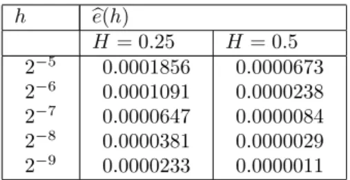
Specifically, the simulations were arranged intoM = 20batches ofK = 100trajectories for each step sizehi =
2−(i+3),withi= 1, ...,6. The significance level was takenα= 0.1.Table I shows the estimated values ofe(h
i)and their
respective90%confidence interval.
h be(h)
H = 0.25 H = 0.5 2−5
2−6
2−7
2−8
2−9
0.0001856 0.0001091 0.0000647 0.0000381 0.0000233
0.0000673 0.0000238 0.0000084 0.0000029 0.0000011
Table I: Uniform discretization errors for the method (7) applied to (10).
Table II show the estimated slopeβb(with its95%confidence interval). This corroborate the usefulness of (7) for the achievement of a desirable deterministic order of convergence.
b
β
H = 0.25 H= 0.5 1.9802±0.0197 1.9938±0.0064
Table II:estimated slopeβb
4. CONCLUSIONS
REFERENCES
[1] Arnold, L.,Random Dynamical Systems, Springer-Verlag, Heidelberg, 1998.
[2] Bharucha-Reid, A.T.,Approximate Solution of Random Equations, North- Holland, New York and Oxford, 1979.
[3] Carbonell F., Jimenez J.C, Biscay R.J, de la Cruz H., The Local Linearization method for numerical integration of random differential equations, BIT Num. Math, 45 (2005), 1-14.
[4] De la Cruz H., Biscay R.J., Jimenez J.C, Carbonell F., Ozaki T.,High Order Local Linearization methods: an approach for constructing A-stable high order explicit schemes for stochastic differential equations with additive noise, BIT Num. Math, 50 (2010), 509-539.
[5] Golub G. H. and Van Loan C. F.,Matrix Computations, The Johns Hopkins University Press, 2nd Edition, 1989. [6] Grune, L. and Kloeden, P. E.,Pathwise approximation of random ordinary differential equation, BIT, 41 (2001) 711–721. [7] Hasminskii, R. Z., Stochastic Stability of Differential Equations, Sijthoff Noordhoff, Alphen aan den Rijn, The Netherlands,
1980.
[8] Jentzen, A. , Kloeden P.,Pathwise Taylor schemes for random ordinary differential equations. BIT Numer. Math., 49 (2009) 113-140.
[9] Kloeden, P. E. and E. Platen, E.,Numerical Solution of Stochastic Differential Equations, Springer-Verlag, Berlin, 1992. [10] Sobczyk, K.,Stochastic differential equations with applications to Physics and Engineering, Kluwer, Dordrecht, 1991.
[11] Soong, T. T.,Random Differential Equations in Science and Engineering, Academic Press, New York, 1974. 16 (1979) 1019-1035.
[12] Vom Scheidt, J., Starkloff, H. J. and Wunderlich, R.,Random transverse vibrations of a one-sided fixed beam and model reduction, ZAMM Z. Angew. Math. Mech., 82 (2002) 847-859.
[13] Sidje, R. B.,EXPOKIT: software package for computing matrix exponentials, AMC Trans. Math. Software, 24 (1998) 130-156. [14] Tiwari, J. L. and Hobbie, J. E.,Random differential equations as models of ecosystems: Monte Carlo simulation approach, Math.
Biosci., 28 (1976) 25-44.
[15] Tsokos, C. P. and Padgett, W. J.,Random Integral Equations with Applications in Sciences and Engineering, Academic Press, New York, (1974).
[16] Wonham, W.M.,Random Differential Equations in Control Theory, In: Probabilistic Methods in Applied Mathematics, Vol. 2, A.T. Bharucha-Reid (Ed.), Academic Press, N.Y., (1971), 31-212.
RESPONSABILIDADE AUTORAL