Modeling underreported infant mortality data with a random censoring poisson model

(1)

Modeling Underreported Infant Mortality

Data with a Random Censoring Poisson

Model

Guilherme Lopes de Oliveira

Departamento de Estat´ıstica - ICEx - UFMG

(2)

Modelando Dados de Mortalidade Infantil

Sub-Registrados usando um Modelo Poisson com

Censura Aleat´

oria

Guilherme Lopes de Oliveira

Orientador: Rosangela Helena Loschi Co-orientador: Renato Martins Assun¸c˜ao

Defesa de disserta¸cão para a obten¸cão do grau de Mestre em Estat´ıstica junto ao Pro-grama de Pós-Gradua¸cão em Estat´ıstica da Universidade Federal de Minas Gerais.

Departamento de Estat´ıstica Instituto de Ciˆencias Exatas Universidade Federal de Minas Gerais

(3)

(4)

“In the end, it’s not the years in your life that count. It’s the life in your years.”

(5)

Acknowledgements

It was a grateful journey and I have to thank everyone who somehow contributed to this achievement.

First, I thank God for giving me health and strength to overcome the problems and to always keep me going ahead.

Second, I thank my parents and brothers for always believe in my potential and never let me give up.

I thank my friends that always motivated me and made me laugh on stress times, specially Ana Cl´audia Silva, Ebert Lima, Rafael Aguiar and Vin´ıcius Lacerda.

My friends and colleagues from the masters course also deserve my thanks for all the shared knowledge, for the constant help during the studies and for the unstresseful

conversations, especially Edson Ferreira, Erick Amorim, Jéssica Almeida, Natália Araújo

and Uriel Silva.

I thank my Professors Rosangela Loschi and Renato Assun¸c˜ao for their trust, support, patience, commitment and for always being encouraging me to continue studying.

To Professors Deise Campos, Leonardo Bastos and Wagner Souza I thank for attend-ing the examination board and contribute to the improvement of the final results of my dissertation.

Also, I thank the professors and staff of the Departamento de Estat´ıstica da UFMG who somehow had helped me along this journey, in especial to Rog´eria Figueiredo and Professor Ela Mercedes de Toscano.

Finally, I thank to CAPES for the scholarship during the Master’s course, to CNPq for the financial support during the undergraduate course and FAPEMIG for the support to participate of conferences throughout my journey at UFMG.

(6)

Abstract

In poor and socially deprived areas, economic, social and health data are typically under-reported. As a consequence, inference using the observed counts for the event of interest will be biased and risks will be underestimated. To overcome this problem, Bailey et al. (2005) propose to consider data from suspected areas as censored information and develop a spatial Bayesian approach for the so-called Censored Poisson model (CPM). However, the CPM assumes that all censored areas are precisely known a priori, which is not a simple task in many practical situations. To account for potential underreporting in an infant mortality dataset, we propose an extension on the CPM by jointly modeling the data generating and the data reporting processes. We assume that observed counts have a Poisson distribution and the underreporting probabilities are associated to an appro-priate logistic model. By doing that, we introduce the Random Censoring Poisson model (RCPM) in which the censoring mechanism is treated as random instead of requiring a previous specification of the censored (underreported) areas. Informative priors on the data reporting process are considered. We also propose a MCMC sampling scheme based on the data augmentation technique. By artificially augmenting the data through latent variables, we facilitate the posterior sampling process. To evaluate the proposed model, we run a simulation study in which such a model is compared with the CPM using different fixed censoring criteria. Also, we apply the proposed model to map the early neonatal mortality rates in Minas Gerais State, Brazil, where data quality is truly poor in many regions.

(7)

Resumo

Em áreas pobres e socialmente mais desfavorecidas, dados econômicos, sociais e de saúde são tipicamente subnotificados. Consequentemente, inferência utilizando as contagens observadas para o evento de interesse será tendenciosa e os riscos inerentes serão subes-timados. Para contornar este problema, Bailey et al. (2005) propõem considerar os dados provenientes de áreas suspeitas como informa¸cões censuradas e desenvolvem uma abordagem Bayesiana espacial para o chamado modelo Poisson Censurado (MPC). Este modelo assume que todas as áreas censuradas são precisamente conhecidasa priori, o que não é uma tarefa simples em muitas situa¸cões práticas. Então, para levar em conta uma potencial subnotifica¸cão em um conjunto de dados de mortalidade infantil, nós propo-mos o modelo Poisson Censurado Aleatoriamente (MPCA) como uma extensão do MPC através da modelagem conjunta dos processos de gera¸cão e de reporta¸cão/registro dos dados em vez de requerer uma pré-especifica¸cão das áreas censuradas. Assume-se que as contagens observadas têm uma distribui¸cão Poisson e as probabilidades de subnotifica¸cão são associados a um modelo log´ıstico apropriado. Distribui¸cõesa priori informativas são consideradas para o processo de reporta¸cão dos dados. Propomos também um esquema de amostragem MCMC baseado na técnica de aumento de dados. Aumentando artificial-mente os dados através de variáveis latentes, nós facilitamos o processo de amostragema

posteriori. Para avaliar o modelo proposto, apresentamos um estudo de simula¸c˜ao em que

tal modelo é comparado com o MPC usando diferentes critérios de censura fixos. Por fim, o modelo proposto é aplicado no mapeamento do risco relativo de mortalidade neonatal precoce no Estado de Minas Gerais, Brasil, onde a qualidade dos dados é verdadeiramente precária em muitas regiões.

(8)

List of Figures

1.1 RR’s estimates of ENM in MG using the SMR (left) and the posterior mean

under the SPM in Ara´ujo and Loschi (2013) (middle); and the Human

Development Index in MG (right) [Source: IBGE 2000]. . . 3

2.1 Comparing the posterior means ofµfor different censoring levelsδ assum-ing prior mean E[µi] =µTi and prior variance V ar[µi] = 100. . . 16

2.2 Comparing the posterior means ofµfor different censoring levelsδ assum-ing prior mean E[µi] = 40.0 and prior variance V ar[µi] = 100. . . 16

2.3 Comparison between the posterior mean of θ and its true value in Case 1. 19

2.6 Comparing the posterior mean of theθ and its true value in Scheme 1. . 23

2.8 Comparing the posterior mean of theθand its true value in Scheme 3. . . 25

3.1 Densities of the prior distributions for λ0 (left) and β (middle); and AI versus logit(pi) = E[λ0]−E[β]AIi (right). . . 41

3.2 Box-plots for the posterior means of θ in Scenario I using Model I, II, IIIand IV from the top to the bottom, respectively. . . 45 3.3 Prior expected mean for the underreporting probabilitiesp(solid line) and

their posterior estimates in Scenario I using Model I: plug-in method

(red dotted line) and posterior proportion of γi = 1, i = 1, ...,75 (black

dotted line). . . 46 3.4 Box-plots for the posterior proportions ofγi = 1, i= 1, ...,75 inScenario

(9)

4.1 Mapping the relative risk of ENM in MG using CPM1 (row 1), CPM2 (row 2) and CPM3 (row 3). In each row: censored regions (left) and posterior medians of the relative risks (right). . . 52

4.2 Posterior mean for the underreporting probabilities (left) and posterior

medians for the relative risk of ENM in MG using RCPM (right). . . 53

4.3 Mapping the relative risk of ENM in MG using RCPM (row 1), CPM1

(10)

List of Tables

3.1 Evaluation metrics for the Monte Carlo study. . . 43

(11)

List of Nomenclatures

Nomenclature Description

AI Adequacy Index

BHM Bayesian Hierarquical model

CAR Conditional Autoregressive model

cpf cumulative probability function

CPM Censored Poisson model

ENM Early Neonatal Mortality

fcd full conditional distribution

FI Functional Illiteracy

HDI Human Development Index

HPD Highest Posterior Density interval

IBGE Instituto Brasileiro de Geografia e Estat´ıstica

IdC Infant Deaths with Ill-defined Cause

MAE Mean Absolute Error

MAPE Mean Absolute Percentage Error

MCMC Markov Chain Monte Carlo

MG Minas Gerais State

MSE Mean Squared Error

MSPE Mean Squared Percentage Error

pf probability function

RCPM Random Censoring Poisson model

RR Relative Risk

SIH Sistema de Informa¸c˜oes Hospitalares

SIM Sistema de Informa¸c˜oes sobre Mortalidade

SINASC Sistema de Informa¸c˜oes sobre Nascidos Vivos

SMR Standardized Mortality/Morbidity Ratio

(12)

Chapter 1 Introduction

Studies related to geographical distribution of disease or mortality incidence and its relationship with potential risk factors have been a rich field for the development of new statistical methods and models. The mapping of the relative risks inherent to this events in small geographical areas is commonly calleddisease mapping and it plays an important role, for instance, in suggesting etiological hypotheses as well as to guide epidemiological control and government intervention. In recent years, powerful and flexible statistical tools have been proposed for disease mapping. A general overview in this topic can be found in Besag (1974), Breslow and Day (1987) and Lawson et al. (1999), to cite a few. Many epidemiological studies focus on early deaths rates because they are indicators

of the population health condition. Among them, the infant mortality rate is

consid-ered of major interest. The mortality rates commonly have their level associated with socioeconomic factors that determine the living conditions and the performance of health services, such as the access and the quality of medical care. To assess the magnitude of the infant mortality rate it is common to use the early neonatal mortality (ENM) rate. The ENM is understood as the infant deaths that occur in the first seven days of life and it is obtained by dividing the number of children that died in the first seven days of life by the total of live births in the period of interest.

In recent decades, the early neonatal mortality has risen its participation in the Brazil-ian infant mortality (Schramm and Szwarcwald, 2000a). Social and economic inequality are the main factors to explain the increase in the death risk of newborns, since these inequalities are usually associated with maternal health problems and difficulties in ac-cessing neonatal care.

(14)

Informa¸c˜oes sobre Mortalidade (SIM) and data related to live births are collected by the

Sistema de Informa¸c˜oes sobre Nascidos Vivos (SINASC) since 1990, both systems were

implemented by the Brazilian Ministry of Health. Due to the data continued collection by the SIM and SINASC, these systems are the best available data sources for monitoring infant mortality in Brazilian municipalities.

However, even with the advances achieved in recent years with relation to data collec-tion systems, in developing countries, such as Brazil, several informacollec-tion are not correctly recorded as they should be. In fact, Schramm and Szwarcwald (2000b), MS-Brasil (2004), Machado et al. (2006), Campos et al. (2007), Frias et al. (2008), Lima et al. (2009) and Guimar˜aes et al. (2013) indicate that information on infant mortality and live births are not correctly recorded in the Brazilian SIM and SINASC systems, mainly in socially deprived areas where the educational level is also precarious. Therefore, the underreport-ing problem may be present in several statistical analysis, especially when one is using Brazilian public health data.

The dataset that motivated this work corresponds to the number of live births and early infant deaths that took place in public hospitals of the 853 municipalities of Minas Gerais State (MG) between 1999 and 2001. Note that, given the serious problems related to underreporting of deaths and births in the SIM and SINASC, we consider data avail-able at the Sistema de Informa¸c˜oes Hospitalares (SIH) of the Brazilian Sistema ´Unico

de Sa´ude (SUS) because Schramm and Szwarcwald (2000b) and Campos et al. (2007)

indicate that SIH provides more reliable information than SIM and SINASC.

According to Campos et al. (2007) and references therein, in MG the early neonatal mortality rate is very high compared to those observed in the other States of Brazilian Southeast and South regions, mainly in more socially deprived areas in the North of MG. Although most of the ENM occurs in hospitals, in MG hospitals are heterogeneously distributed around the State, making the access to health care in socially deprived areas quite difficult. Also because of this, data on ENM are usually underreported and the quality of information produced in the State is quite poor. In fact, MG is the only state in the Brazilian Southeast region where the official infant mortality rates are estimated by the Instituto Brasileiro de Geografia e Estat´ıstica (IBGE) using indirect methods (MS-Brasil (2004) and Ortiz (2000)).

Figure 1.1 presents a first study involving our dataset of interest. The 853 munici-palities of Minas Gerais State are grouped into 75 regions in order to avoid regions with very small or zero counts, which leads to unstable estimates for the mortality rates as discussed in Assun¸c˜ao et al. (1998).

(15)

of ENM in Minas Gerais State obtained by fitting the standard Poisson model (see Section 2.1). The results indicate that northern regions of MG experience the lowest ENM rates, which are close to those observed for highly developed countries. This estimates are inconsistent with the expected by epidemiologists for those regions, because North and Northeast of MG are poorly developed regions and they present the worst social indicators in the State, as can be seen in Figure 1.1 (right) that displays the Human Development Index (HDI) in 2000 for the n= 75 regions of MG.

The standard Poisson model does not account for the spatial correlation among neigh-bouring areas. Considering such type of correlation is a strategy commonly used to smooth and to overcome inconsistencies in the mortality rates estimation. Ara´ujo and Loschi (2013) mapped the relative risks of ENM in Minas Gerais State using a Bayesian approach for the Spatial Poisson model that includes covariates and spatially structured random effects (see Section 2.1.1). The posterior means for the RR obtained under such a model are displayed in Figure 1.1 (middle).

Despite this more sophisticated model considers the spatial correlation between neigh-boring areas, it does not overcome the underestimation of the relative risk in the poorest regions in North and Northeast of MG, since the estimates in these regions remained below than the expected and similar to those seen in highly developed countries. It is noticeable from Figure 1.1 that the maximum likelihood (left)and the Bayesian (middle) estimates for the ENM in MG are quite similar. Such results raise some doubts regarding the quality of early infanty mortality and live births data collected from the SIH, as had already been observed with relation to data from SIM and SINASC.

[0,0.5) [0.5,1) [1,1.5) [1.5,2.5) [2.5,5.5]

[0.42,0.516) [0.516,0.59) [0.59,0.61) [0.61,0.63) [0.63,0.7]

Figure 1.1: RR’s estimates of ENM in MG using the SMR (left) and the posterior mean

under the SPM in Ara´ujo and Loschi (2013) (middle); and the Human Development

(16)

In fact, a possible explanation for those inconsistencies in the ENM’s relative risk estimation for the northern regions of MG is the occurrence of underreporting on the SIH’s data, as discussed in Campos et al. (2007). As pointed out by those authors, the underreporting of live births and early infant deaths discloses the socioeconomic, geographical and cultural inequalities as well as the marginalization of population groups in MG. Consequently, official statistics for the State do not measure the death risk of newborns in all its magnitude, making difficult an adequate epidemiological analysis.

In addition to Campos et al. (2007), Andrade et al. (2006) also indicate a possible relationship between socioeconomic status and quality of mortality information when analyzing data from Paran´a State, concluding that in areas facing socioeconomic prob-lems the occurrence of underreporting is quite plausible. Also analyzing Brazilian public health data, Bailey et al. (2005) discuss about underreporting in leprosy incidence in Olinda city, Pernambuco State.

The important point is that, if underreporting occurs and it is not accounted for, in-ference using the observed counts will be biased and, consequently, the inherent relative risks will be underestimated. Whatever the source, underreporting will invalidate the assumptions of the standard Poisson model which is conventionally used in count data problems. Therefore, when using data with suspected underreporting, it is quite impor-tant to use models that account for it. Though information about unreported events is missing, underreporting is different from the usual concept of missing data. In usual missing data problems, information that data are missing is available and hence can be incorporated in the analysis, whereas for an unreported event no information at all is generated.

To overcome the underreporting problem in their leprosy incidence dataset, Bailey et al. (2005) propose to consider data with suspected underreporting as censored infor-mation and use a Censored Poisson model (CPM) that takes into account the spatial association among neighboring areas. The big challenge in considering the CPM is the prior definition of all censored (underreported) areas that is needed in its construction. Usually, information about the censored areas are obtained indirectly and ad-hoc proce-dures are considered to determine them. For their particular application, Bailey et al. (2005) use a social deprivation indicator as a criterion for considering data from certain regions as unreliable data (underreported data).

(17)

that allows for underreporting in the counts. It is assumed that the true (but unobserved) absent counts are generated by a Poisson process and the reporting/non-reporting is independent for each event. As far as we know, that is the only approach proposed in the Literature for jointly model the data generating and the data reporting processes in the context of underreported count data.

Dvorzak and Wagner (2015) extend the model from Winkelmann (1996) by incorpo-rating both cluster analysis and Bayesian variable selection to estimate risk of cervical cancer death using underreported data. In their extension of Winkelmann (1996)’s model, the intensity of the Poisson process and the reporting probability are both related to a set of potential covariates through the specification of regression models. Identification of the proposed model requires additional information, which can be provided either by additional data on the reporting process (validation data), parameter restrictions or informative prior on parameters, e.g., provided by experts.

In this work, we introduce a different approach for jointly model the data generating and the data reporting processes in the context of underreported data. We do that by extending the CPM presented in Bailey et al. (2005). Basically, we introduce on the CPM a random mechanism to specify the censored (underreported) areas, instead of using a fixed vector to previously indicate those censored ones. Therefore, as opposed to what is found in Bailey et al. (2005), we can now estimate the probability of the information in each area being censored at the same time that the relative risk for the event of interest is being estimated. We call the proposed model by Random Censoring Poisson model (RCPM). Therefore, the RCPM arises as an alternative model to that one proposed in Dvorzak and Wagner (2015) to handle underreported count data.

We develop an algorithm to sample from the posterior distribution that relies on the data augmentation strategy (Tanner and Wong (1987) and Chib (1992)), which simplify substantially the posterior sampling process. We run a Monte Carlo simulation study for comparing the RCPM that is been proposed with the CPM from Bailey et al. (2005), in which the censored areas must be previously specified. We consider different scenarios for generating the datasets in such a simulation study. Moreover, we consider the proposed model to analyze the ENM’s data in Minas Gerais State. Results are compared with those ones obtained by using the CPM under three different fixed censoring criteria proposed in Oliveira and Loschi (2013).

(18)

(19)

Chapter 2 Background and Theoretical

Framework

The goal of this chapter is to introduce the basic elements needed to understand the problem we have at hand, a solution already presented in the Literature and the solution proposed in Chapter 3. Firstly, some methods widely used in the context of disease mapping will be discussed, including the Spatial Poisson model (Besag et al., 1991). We then present the Censored Poisson model (CPM) proposed in the Literature to model underreported count data. Some simulation studies involving the CPM will be performed in order to better understand its advantages and disadvantages.

We start highlighting that the use of maps to display the geographical variability of the relative risk (RR) inherent to certain events as disease or mortality is quite popular nowadays. The statistical problem of searching for efficient models to appropriately map-ping those quantities has received considerable attention recently, particularly because this kind of maps can help us to detect areas where the event is especially prevalent and also for detecting previously unknown risk factors. The risk may reflect actual deaths due to a disease (mortality) or, if it is not fatal, the number of people who suffer from a disease (morbidity) for the population at risk in a certain period of time. Hence, for doing such analysis, basic data must include information about the population at risk and the number of cases in each area.

The term disease mapping is concerned with the estimation of the true underlying

(20)

methods related to the former. Readers interested in clustering analysis in the disease mapping context may see, for instance, Besag et al. (1991), Holmes et al. (1999),Knorr-Held and Best (2001), Denison and Holmes (2001), Hegarty and Barry (2008) and Teixeira et al. (2015).

The type of data more commonly encountered in disease mapping is the count by area

or areal data, since in most cases the event exact locations are unknown due to medical

confidentiality, for instance. Throughout this work only areal data will be considered. To establish notation, along this workYi andEi will denote, respectively, the observed

and the expected number of cases in area i = 1, ..., n. The Yi is a random variable that

assumes the value yi after observation. The quantityEi is fixed and a known function of

the number ni of individuals at risk in area igiven by

Ei =ni

 

P

i

yi

P

i

ni



=nir,

wherer =P_iyi[Pini]−

1

denotes the overall disease (mortality) rate in the whole region. This chapter is organized as follows. In Section 2.1 we present the standard and the Spatial Poisson models. In Section 2.2 the Censored Poisson model (CPM) is discussed and presented as an alternative approach to handle underreported count data. Section 2.3 presents some simulation studies involving the CPM.

2.1 Poisson Model

To assess the status of an area with respect to the incidence of an event, it is convenient to firstly obtain the expected incidence given the population at risk in the area and then compare it with the observed incidence. This approach has been traditionally used in the analysis of counts within areas or sub-regions. The ratio of observed to expected counts in each area is calledStandardized Mortality/Morbidity Ratio (SMR) and it is given by

SM Ri =

yi

Ei

, (2.1)

for i = 1, ..., n. The ratio in expression (2.1) gives a naive estimator of the relative risk (RR) in area i (Breslow and Day, 1987).

(21)

occur in areas with the small populations. Therefore, SMR can be useless for mapping the desired relative risks. Mapping based on that quantity can also fail when dealing with underreported data, since the regions of greatest potential interest are usually small and often associated with the less reliable data. Actually, the SMR is not an appropriate choice in a great number of situations.

Alternatively, to estimate the relative risks we can assume that the observed count of cases Yi in each area i has a Poisson distribution with mean µi = Eiθi, where θi

denotes the true relative risk associated to this area. In that case, if Y = (Y1, ..., Yn) are

independent, given θ = (θ1, ..., θn), so that

Yi|θi ind

∼ Poisson(Eiθi); (2.2)

and, if θi is taken as a fixed effect associated to area i, then the maximum likelihood

estimator for θi is the SM Ri given in expression (2.1). Consequently, this approach is

not a good choice for mapping rare events data. Despite this, some inference results considering parameter θi as a fixed effect under the standard Poisson model presented in

(2.2) can be found in Breslow and Day (1987); such as classical confidence intervals and hypothesis tests. In Section 2.1.1, we briefly discuss about an efficient strategy to better estimate the relative risks θ that consists in considering the spatial correlation among the neighbouring areas.

2.1.1 Spatial Poisson Model

As previously discussed, the main goal in disease mapping is to research for methods capable to produce more reliable maps of the underlying geographical variation in disease or mortality risks. According to Bailey (2001), a good method must be capable to reduce the excess of local variability as well as to correct the variations produced by risk factors or population differences such as age, sex and so on.

To deal with this issue, some smoothing of the realtive risks is incorporated into the standard Poisson model in (2.2) by takingθi as a random effect (or a function of random

effects). This strategy allows for overdispersion in the standard Poisson model caused, for instance, by unobserved covariates or confounding factors (Molli´e (1995) and Clayton and Bernardinelli (1996)).

(22)

model (BHM), where a prior distribution is assigned to each θi (e.g., see Breslow and

Day (1987)).

Therefore, in Bayesian disease mapping, a BHM combines two types of information: the one provided by the observed counts in each region, usually summarized by the Poisson likelihood π(Y |θ), and the prior information about the relative risk behavior in the overall map, summarized by its prior distribution π(θ). Therefore, π(θ) should reflect the prior knowledge about the variation in relative risk over the map Bernardinelli et al. (1995).

As in model (2.2), assume that the counts Y in the ndifferent areas are independent given θ, so that

Yi|θi ind

∼ Poisson(Eiθi).

The Spatial Poisson model suggested by Besag et al. (1991) considers the relative risk

θi as a function of random effects to allow for overdispersion produced by unobserved

covariates or confounding factors as well as to reflect the explicit spatial dependence among Y. It is assumed that

logµi = logEi+ logθi = logEi+υi+si, (2.3)

where υi and si are, respectively, a non-spatially structured and a spatially structured

random effect. The quantity υi accounts for a dependence among the counts Y induced

by unmeasured covariates or confounding factors. Typically, υi does not account for

an explicit spatial dependence among the counts which may arise, for instance, through lesser variability of rates on neighbouring densely populated urban areas as opposed to sparsely populated rural areas or through an infectious etiology of the disease. Thus, the spatially structured random effectsi is introduced into the model to describe such spatial

association. Details on this model can be found, e.g., in Besag et al. (1991), Molli´e (1995) and Clayton and Bernardinelli (1996).

The typical prior assumption for υi is the Normal distribution N(µυ, συ2), with the

hyperpriors being a Normal distribution for the hyperparameter µυ and a Gamma

dis-tribution for the precision hyperparameter τ2

υ = 1/σ

2

υ. The prior specification for s =

(s1, ..., sn) must disclose the spatial dependence among the areas. Usually, it is assigned

a Conditional Autoregressive model (CAR) as prior distribution fors, in which the mean value for the marginal distribution of si is a weighted average of the neighboring random

effects and the varianceσ2

s controls the strength of this local spatial dependence. A vague

Gamma distribution is commonly assumed for the precision hyperparameter τ2

s = 1/σ

2

s.

(23)

found, for instance, in Besag and Kooperberg (1995) and Banerjee et al. (2004).

The basic Bayesian hierarchical model in (2.3) can be extended by including k covari-ates, (xi1, ..., xik), related to suspected risk factors and so that

log µi = log Ei+ k

X

j=1

βjxij +υi+si, (2.4)

whereµi, Ei, υi andsi are defined as before. The parameterβj is a fixed effect associated

to the j-th covariate, j = 1, ..., k, and reflects the influence of this covariate on the log relative risk given by log θi =P

k

j=1βjxij +υi +si. A constant term β0 can also be considered, so that log θi =β0+Pk_j₌₁βjxij+υi+si. Usually it is assumed that the fixed

effects β = (β0, β1, ..., βk) are independent and identically distributed (iid) according to

a non-informative (vague) prior distribution, e.g., a zero centered multivariate Normal distribution having a diagonal covariance matrix with large variances. MCMC methods are used to sample from the joint posterior distributionπ(β0,β,s|Y). Further details and variations on this basic modeling framework may be found in many published examples of ecological and epidemiological studies (e.g. see Lawson et al. (1999) and references therein).

2.2 Censored Poisson Model

The Censored Poisson model (CPM) was firstly proposed by Terza (1985). Despite being mainly considered for modeling count data that exhibit either over or under-dispersion (Cameron and Trivedi, 1998) it has also been considered for modeling censored data as discussed in Famoye and Wang (2004), where a generalization of the CPM is developed to handle general types of censoring. By simplicity and for our purpose, we only consider right censored data.

As in the previous models, let Yi be the count for the event of interest occurred in

area i, i= 1, ..., n, and assume that

Yi|µi ind

∼ Poisson(µi).

The assumption that all Yi are completely observed is unrealistic in many count data

applications. Rather, it is possible that the reported number of eventsyi constitutes only

a fraction of all events and, thefore, data are underreported.

To built the CPM, consider that some observable variables Yi are not completely

(24)

i-th observation yi, the complete information is considered, that is, Yi =yi. However, if

a censoring occurs for the i-th observation, the true number of cases associated to this observation is considered at least equal to the observed value, i.e., Yi ≥yi. Denote by γi

the censoring indicator variable such that

γi =

(

1, if information at area i is censored,

0, otherwise.

In Famoye and Wang (2004)’s approach, the censoring vector γ = (γ1, ..., γn) must be

known and fixed a priori.

Assuming independence between the counts Yi, given γi and µi, for i = 1, ..., n; and

also assuming that the censoring mechanism is independent of the number of events in each area, Famoye and Wang (2004) built the likelihood function that characterizes the CPM as being

L(µ;y,γ) =

n

Y

i=1

n

fYi|µi(yi)

1−γi

1−FYi|µi(yi−1)

γio

=

n

Y

i=1

(

eµiµyi

i

yi!

1−γi X

y≥yi

eµiµy

i

y!

!γi)

. (2.5)

where fYi|µi and FYi|µi denote, respectively, the probability function (pf) and cumulative probability function (cpf) of a random variable with distribution Poisson(µi).

Bailey et al. (2005) propose to consider the CPM to handle underreported leprosy data from Olinda city, Pernambuco State, Brazil. Basically, the underreported counts are treated as censures considered to be lower bounds to the real (but unobserved) counts. In such approach, the censoring indicator vector γ= (γ1, ..., γn) is fixed a priori, that is,

we must precisely know all the areas whose counts are underreported. However, censored observations are not obviously identified as in Survival Analysis studies. In a general context, several criteria may be available to partitioning the observations as censored or non-censored. In their particular application, Bailey et al. (2005) make such a partition of the areas using values of a social deprivation indicator, based on the fact that the observations considered most unreliable are those from the poorer areas. The occurrence rate of leprosy is taken as being

log µi = log Ei+β0+βxi+υi+si,

(25)

centered proportion of the population at risk in thei-th area with monthly income below one minimum legal wage and, respectively, si and υi are the spatially and non-spatially

structured random effects in each census tract.

For posterior inference the MCMC methodology is considered. For the non-spatially structured random effects, υi, are assumed independent Normal distributions with zero

mean and variance σ2

υ. The joint prior distribution for the spatially structured random

effects,s= (s1, ..., sn), is taken as a Gaussian intrinsic CAR model, where the mean value

for si|sj, for all j 6=i, is a weighted average of the neighbouring random effects and the

variance,σ2

s, controls the strength of this local spatial dependence. The neighbourhoods

are defined by simple binary adjacency weights, that is, trough a proximity matrix W, in which the entries ωij = 1 if areaishares a common boundary with area j and ωij = 0

otherwise. An improper flat Uniform prior distribution is assigned for the intercept β0 and a flat Gamma hyperprior distribution is assumed for the precisions τ = 1/σ2

θ and

φ= 1/σ2

υ. For parameters β it is used a vague zero mean Normal distribution.

Bailey et al. (2005) concluded that CPM provided reasonable estimates for the leprosy rates in Olinda. However, it is not trivial how to define the censored areas in real problems like that discussed in Bailey et al. (2005). An ideal model should also infer about the censored areas. For that purpose, in Chapter 3 we introduce a Poisson model that allows us to make inference about the censored areas at the same time that we infer about the inherent relative risks. Before doing that, we will perform some simulation studies involving the CPM in order to better evaluate the quality of its estimates. Such studies for the CPM in the context of underreported data is not presented in Bailey et al. (2005) neither in other papers. The details and results for the simulation studies are presented in Section 2.3.

2.3 Simulation Studies on the Censored Poisson Model

(26)

were implemented in R 3.1.3 (www.r-project.org) and OpenBUGS (www.openbugs.net) languages. In all case, we run the MCMC for 85000 iterations, discarding the first 20000 draws as a burn-in period and considering a lag 13 to avoid correlation. Thus, we consider a sample of size 5000 for making posterior inference. Also, in all figures presented throughout this section the symbols + and ◦ will represent the censored and non-censored areas, respectively.

2.3.1 Simulation 1: The

Data Censoring Level

Effect

Our interest here is to investigate the behavior of the relative risk estimates for different censoring levels in the observed counts under the CPM. Assume that the event count y∗

i

in area i= 1, ...,75 is generated from a Poisson distribution such that

Yi∗|µi ind

∼ P oisson(µi),

where µi is so that

µi =

    

70, i= 1, ...,25 30, i= 26, ...,50·

10, i= 51, ...,75,

and denote by µT _{this true values of}_µ _{used to generate the data.}

We assume 21 censored areas according to the following censoring indicator vector

γi =

(

1, i= 1, ...,7 and i= 26, ...,32 and i= 51, ...,57

0, otherwise. (2.6)

Let δ be the censoring level desired, i.e., the proportion of the generated value y∗

i

that will be correctly reported in each censored area. In this case, (1−δ)×100% of the information will be missed (underreported) if the area is a censored one. Thus, the counts yi in censored areas are built by multiplying the generate value y∗i byδ. Since the

count must belong to the set of positive integer numbers, Z+, in all censored area the observation yi is taken as the smallest integer greater or equal than the value obtained

from the multiplication y∗

i ×δ, that is,

yi =

(

⌈y∗

i ×δ⌉, if γi = 1

y∗i, if γi = 0.

(27)

scenarios.

For modeling the simulated datasets, we fit the Censored Poisson model given by

Yi|γi, µi ind

∼ CP(µi)

µi ind

∼ Gamma(α, φ),

where by notation CP(µi) we mean that observation Yi has a Poisson distribution with

rateµiand, givenµiandγi, the contribution of this observation for the likelihood function

corresponds to the i-th term of the function in (2.5).

The censored areas are pre-fixed as required in Bailey et al. (2005) and assumed to be those areas indicated in (2.6). We assume two different prior specifications forµi. For

results presented in Figure 2.1 we choose a Gamma(α, φ) so that a priori E[µi] = µTi

and V ar[µi] = 100, whereas in Figure 2.2 we choose α andφ such thatE[µi] = 40.0 and

V ar[µi] = 100, for i= 1, ...,75. By doing this, despite of the large variance, we have one

case in which the prior distribution represents well the generated data (E[µi] = µTi , for

alli) and another case in which the prior distribution has the same shape for all regions (E[µi] = 40.0, for all i).

Figures 2.1 and 2.2 compare the posterior means of µ obtained for each censoring

level. The estimates of µ in non-censored areas (◦) are not influenced by the censoring level being quite close in all cases. It is also noticeable that better estimates are achieved in non-censored areas when the prior distribution is centered on µT (Figure 2.1) than when the prior distribution is centered on an arbitrary value for all areas (Figure 2.2). In censored regions (+), the estimates of µare more similar when the associated censoring levels in the data are closer. From Figure 2.1, we noticed that the posterior means in censored areas tends to overestimate the true relative risk, mainly in datasets in which a lower censoring level is assumed. Figure 2.2 discloses that the posterior mean in censored areas tends to approximate of the prior mean. We also noted that the influence of prior information depends on the censoring level: as the censoring level increases, the influence of the prior mean also increases.

(28)

20 40 60 80 20 40 60 80 Censure 10% Censure 20%

20 40 60 80

20 40 60 80 Censure 10% Censure 30%

20 40 60 80

Figure 2.1: Comparing the posterior means ofµfor different censoring levelsδ assuming prior mean E[µi] =µTi and prior variance V ar[µi] = 100.

20 30 40 50 60 70 80

20 30 40 50 60 70 80 Censure 10% Censure 20%

20 30 40 50 60 70 80

20 30 40 50 60 70 80 Censure 10% Censure 30%

20 30 40 50 60 70 80

20 30 40 50 60 70 80 Censure 10% Censure 60%

20 30 40 50 60 70 80

20 30 40 50 60 70 80 Censure 20% Censure 30%

20 30 40 50 60 70 80

20 30 40 50 60 70 80 Censure 20% Censure 60%

20 30 40 50 60 70 80

20 30 40 50 60 70 80 Censure 30% Censure 60%

(29)

2.3.2 Simulation 2: The Proportion of Censored Areas Effect

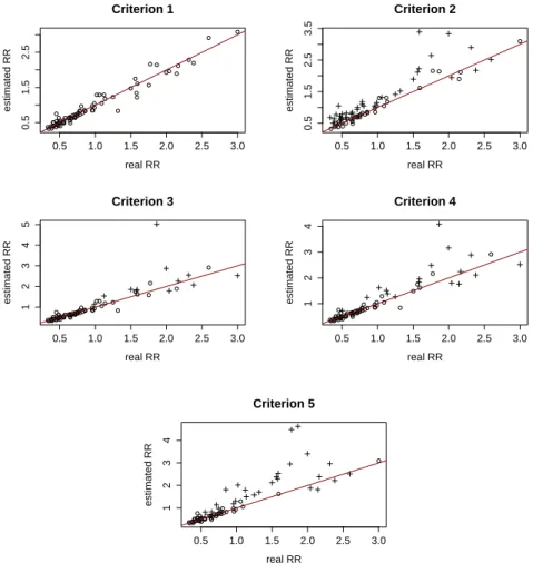
In this section we consider five censoring criteria that induces different proportions of censored areas in the data. We fit three different Censored Poisson models such that, in Case 1, the relative risk (RR) is considered to be a spatially structured random effect, in Case 2, the RR is considered to be a spatially non-structured random effect and, in Case 3, the RR is a function of spatially and non-spatially structured random effects. Therefore, at the same time, we are evaluating the effect of the number of censored areas and the effect of including or not including a spatial random effect for modeling the relative risks θ.

Considering the known latitudes (denoted by Lat) inherent to the n = 75 regions of MG map, data are generated assuming an increasing relative risk from the South to the North, so that θi = exp{a+bLati}, for i = 1, ...75. To determine the values of a and b,

we fixed that the region with the smallest latitude has θ = 0.3 and the region with the greatest latitude has θ = 3.0 and solve the following equation system

(

exp{a+bmin(Lati)}= 0.3

exp{a+bmax(Lati)}= 3.0,

(2.7)

which provides a= 5.71 and b= 0.31.

Assuming we have access to the expected number of cases in areai= 1, ...,75, denoted

Ei, the count in each area is generated from a Poisson distribution such that

Yi∗|θi ind

∼ P oisson(Eiθi). (2.8)

Five fixed censoring criteria are considered. They differ from each other due to the proportion of censored areas. We consider a scenario without censored areas (Criterion 1), the Criterion 2 that consider almost 50% of the areas as being censored and the three censoring criteria proposed by Oliveira and Loschi (2013) (denoted by Criterion 3, 4 and 5). These censoring criteria are summarized below with their respective proportion of censored areas given in parentheses.

Criterion 1: no area is censored (0%)

Criterion 2: γi = 1 for i= 1, ...,7,16, ...,22,31, ...,37,46, ...,52,61, ...,67 (47%)

Criterion 3: γi = 1 ifHDIi ≤HDI15% (16%)

Criterion 4: γi = 1 ifAIi ≤20.0 (23%)

(30)

where HDIi represents the Human Development Index in 2000 for the regions of MG,

AIi is the Adequacy Index proposed by Fran¸ca et al. (2006) which measures the quality

of mortality information in MG, F Ii denotes the proportion of Functional Illiteracy in

each region of the State, IdCi is the proportion of Infant Deaths with Ill-defined Cause

in these regions and Xα% denotes the α-th percentile of the quantity X.

In this study we only consider the censoring level δ = 0.7, that is, the counts yi

in censored areas are given by ⌈y∗

i ×0.7⌉, where yi∗ is the value generated from (2.8).

To model the simulated datasets we fit the Censored Poisson model as described in the following Cases 1, 2 and 3. In all cases. The censoring indicator vectors used to generate the data are considered in the modeling, that is, the correct censoring criteria used to generate the datasets are considered in the fitted models.

Case 1: Spatially Structured Random Effect Model

The CPM considered here assumes that θi = exp{si}, where si represents a spatially

structured random effect, such that

Yi|γi, µi ind

∼ CP(µi)

µi = Eiexp{si}

s|W,ξ ∼ CAR(W,ξ),

where W and ξ are, respectively, the proximity matrix inherent to the map and the

hyperparameters associated to the CAR model (Banerjee et al., 2004).

(31)

0.5 1.0 1.5 2.0 2.5 3.0

0.5

1.5

2.5

Criterion 1

real RR

estimated RR

0.5 1.0 1.5 2.0 2.5 3.0

0.5

1.5

2.5

3.5

Criterion 2

real RR

estimated RR

0.5 1.0 1.5 2.0 2.5 3.0

1

2

3

4

5

Criterion 3

real RR

estimated RR

0.5 1.0 1.5 2.0 2.5 3.0

1

2

3

4

Criterion 4

real RR

estimated RR

0.5 1.0 1.5 2.0 2.5 3.0

1

2

3

4

Criterion 5

real RR

estimated RR

Figure 2.3: Comparison between the posterior mean of θ and its true value in Case 1.

Case 2: Spatially non-Structured Random Effect Model

Assume now that in the CPM we model the relative risk in each area as being θi =

exp{υi}, where υi represents a spatially non-structured random effect, so that

Yi|γi, µi ind

∼ CP(µi)

µi = Eiexp{υi}

υi iid

∼ N ormal(0.0,2.0),

(32)

Case 1 - we notice that, in general, the overestimation is lesser than that observed in Case 1 in relation to the extreme estimates for the relative risks. This apparent superiority of the model with a non-spatial random effect (Case 2) in relation to the model with a spatial random effect (Case 1) is an unexpected result, because the data were generated assuming an increasing relative risk from the South to the North, which establishes a kind of spatial structure in the map. However, we must consider that the spatial structure assumed in Case 1 takes into account the information in neighbouring areas to estimate the risk in each area, which seems to affect the estimates, mainly in censored areas in which the most neighbouring areas are also censored - in general, a greater overestimation (extreme values) is noted for such areas.

0.5 1.0 1.5 2.0 2.5 3.0

0.5

1.5

2.5

Criterion 1

real RR

estimated RR

0.5 1.0 1.5 2.0 2.5 3.0

0.5

1.5

2.5

Criterion 2

real RR

estimated RR

0.5 1.0 1.5 2.0 2.5 3.0

0.5

1.5

2.5

3.5

Criterion 3

real RR

estimated RR

0.5 1.0 1.5 2.0 2.5 3.0

0.5

1.5

2.5

Criterion 4

real RR

estimated RR

0.5 1.0 1.5 2.0 2.5 3.0

0.5

1.5

2.5

Criterion 5

real RR

estimated RR

(33)

Case 3: Spatially Structured and non-Structured Random Effects Model

In this last case, the CPM fitted to analyze the datasets considers thatθi = exp{υi+si},

where υi and si represents the spatially non-structured and structured random effect,

respectively, and now

Yi|γi, µi ind

∼ CP(µi)

µi = Eiexp{υi+si}

υi iid

∼ N ormal(0.0,2.0)

s|W,ξ ∼ CAR(W,ξ).

Figure 2.5 shows the comparison between the posterior mean of θ and its true value for each censoring criteria. The posterior estimates of RR are quite similar to those obtained in Case 2, showing that the spatially structured random affect does not play an important role in the relative risks estimation for the generated scenarios.

0.5 1.0 1.5 2.0 2.5 3.0

0.5

1.5

2.5

Criterion 1

real RR

estimated RR

0.5 1.0 1.5 2.0 2.5 3.0

0.5

1.5

2.5

Criterion 2

real RR

estimated RR

0.5 1.0 1.5 2.0 2.5 3.0

0.5

1.5

2.5

Criterion 3

real RR

estimated RR

0.5 1.0 1.5 2.0 2.5 3.0

0.5

1.5

2.5

Criterion 4

real RR

estimated RR

0.5 1.0 1.5 2.0 2.5 3.0

0.5

1.5

2.5

3.5

Criterion 5

real RR

estimated RR

(34)

2.3.3 Simulation 3: The Clusterization Effect

In this section we evaluate the behavior of the relative risk estimates considering the

existence of clusters in the n = 75 regions of MG map. Those clusters induce a

par-tition of the map, denoted by ρ. Assume the existence of five independent clusters

Cj, j = 1, ...,5, such that ρ = {C1 = (1, ...,15),C2 = (16, ...,30),C3 = (31, ...,45),C4 = (46, ...,60),C5 = (61, ...,75)}. Also assume that such a partition induces the existence of

θρ= (θC1, θC2, θC3, θC4, θC5) such that the countsYi in areas belonging to a given clusterCj

are independent with θi d

=θk for all (i, k)∈ Cj. That is, the counts Yi in areas belonging

to cluster Cj are independent and identically distributed.

As before, assume that the expected number of cases in areai,Ei, is available. Thus,

the count y∗

i in each area is generated from a Poisson distribution given by

Y_i∗|θi ind

∼ P oisson(Eiθi),

where

θi =

              

7.4 for all i∈ C1 2.7 for all i∈ C2 1.0 for all i∈ C3 0.6 for all i∈ C4 0.4 for all i∈ C5

Denote the true value of θi used to generate the data by θTi . We only consider the

censoring level δ = 0.7, which means that the counts yi in censored areas are given by

⌈y∗i ×0.7⌉(see Section 2.3.1). The censoring mechanism used to generate the datasets is

fixed and corresponds to the five censoring criteria presented in Section 2.3.2. To analyze the simulated datasets, we fit the following model

Yi|γi, θi ind

∼ CP(Eiθi)

θi ind

∼ Gamma(αi, φi),

The study is divided into four schemes. The difference among the schemes is due to the Gamma prior distribution assumed to model the uncertainty about the relative risks

(35)

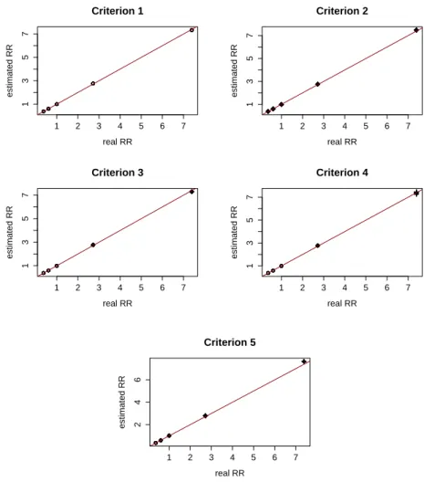
Scheme 1: Using Informative Priors and Informing the Correct Partition

In this first scheme, to built the prior distribution of θi we choose αi and φi so that a

priori E[θi] = θTi and V ar[θi] = 100 for all i. Moreover, the exact partition ρ = {C1 =

(1, ...,15),C2 = (16, ...,30),C3 = (31, ...,45),C4 = (46, ...,60),C5 = (61, ...,75)}is reported to the model.

Comparisons between the posterior mean of relative risks θ and their true values for each censoring criteria are shown in Figure 2.6. In all criteria, for both non-censored (◦) and censored (+) areas, the estimates are exactly equal to their true values or quite close to them. Such a result indicates that we can obtain optimal posterior estimates for the relative risksθ if we provide a good prior information for it as well as a good information about the partition structure inherent to the map.

1 2 3 4 5 6 7

1

3

5

7

Criterion 1

real RR

estimated RR

1 2 3 4 5 6 7

1

3

5

7

Criterion 2

real RR

estimated RR

1 2 3 4 5 6 7

1

3

5

7

Criterion 3

real RR

estimated RR

1 2 3 4 5 6 7

1

3

5

7

Criterion 4

real RR

estimated RR

1 2 3 4 5 6 7

2

4

6

Criterion 5

real RR

estimated RR

(36)

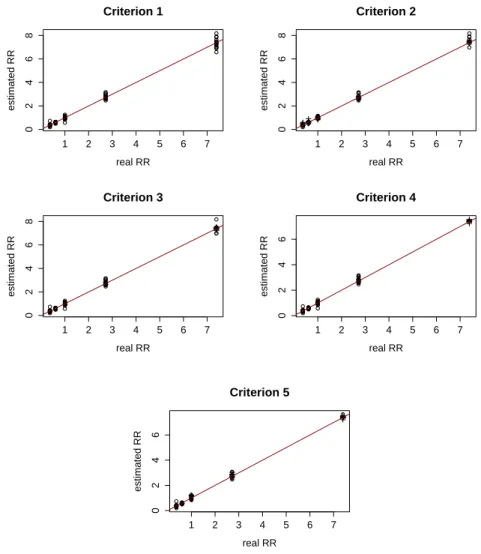
Scheme 2: Using Informative Priors and not-Informing the Correct Partition

As in Scheme 1, here we built the prior distribution of θi choosing αi and φi so that a

priori E[θi] = θiT and V ar[θi] = 100 for all i. However, instead of reporting the correct

partition to the model, we report ρ = {C1 = (1),C2 = (2),C3 = (3), ...,C75 = (75)}, i.e., the model will estimate the parameters θi by treating each area as a single cluster.

The posterior mean of the relative risks θ are compared to their true values in Figure 2.7 for each censoring criteria. In general, for both non-censored (◦) and censored (+) areas, the posterior estimates are close to their true values although not so close as seen in Scheme 1. Anyway, we have some evidence that, if we provide a good prior information for all θi, the relative risks will be well estimated even when the correct partition of the

map is not identified.

1 2 3 4 5 6 7

0

2

4

6

8

Criterion 1

real RR

estimated RR

1 2 3 4 5 6 7

0

2

4

6

8

Criterion 2

real RR

estimated RR

1 2 3 4 5 6 7

0

2

4

6

8

Criterion 3

real RR

estimated RR

1 2 3 4 5 6 7

0

2

4

6

Criterion 4

real RR

estimated RR

1 2 3 4 5 6 7

0

2

4

6

Criterion 5

real RR

estimated RR

(37)

Scheme 3: Using non-Informative Priors and Informing the Correct Partition

To built the prior distribution of θi in this scheme, we chooseαi and φi so that a priori

E[θi] = 5.0 and V ar[θi] = 100 for all i. Moreover, assume that the correct partition

ρ= {C1 = (1, ...,15),C2 = (16, ...,30),C3 = (31, ...,45),C4 = (46, ...,60),C5 = (61, ...,75)} is reported to the model.

Figure 2.8 displays the comparison between the posterior mean of θ and its true

value for each censoring criteria. Except under Criterion 4, for both non-censored (◦) and censored (+) areas, in most areas the estimates are equal to the true values or quite close to them, as observed in Scheme 1.

1 2 3 4 5 6 7

1

3

5

7

Criterion 1

real RR

estimated RR

1 2 3 4 5 6 7

1

3

5

7

Criterion 2

real RR

estimated RR

1 2 3 4 5 6 7

1

3

5

7

Criterion 3

real RR

estimated RR

1 2 3 4 5 6 7

1

2

3

4

5

Criterion 4

real RR

estimated RR

1 2 3 4 5 6 7

2

4

6

Criterion 5

real RR

estimated RR

Figure 2.8: Comparing the posterior mean of the θand its true value in Scheme 3.

(38)

under Criterion 4 and the posterior mean for the RR in areas belonging to these clusters remaining quite close to its true value, as observed in all other censoring criteria.

Therefore, there is an evidence that the prior distribution has a strong influence on the posterior estimates of the relative risk in clusters where 100% of the areas are censored, even if the partition inherent to the map is correctly identified. The influence of the prior choice is minimized if the cluster contains at least one non-censored area and the correct partition is reported to the model.

Scheme 4: Using non-Informative Priors and not-Informing the Correct

Par-tition

In this last Scheme, we perform a simulation study in whichαi and φi are chosen so that

a priori E[θi] = 5.0 and V ar[θi] = 100 for all i and, at the same time, we report to the

model that ρ={C1 = (1),C2 = (2),C3 = (3), ...,C75= (75)}, i.e., the model will estimate

θ by treating each area as a single cluster. Thus, we do not provide to the model a good prior information for the relative risks neither the correct partition inherent to the map. Results are shown in Figure 2.9 for each censoring criteria. The estimates in non-censored areas (◦) are close to their true values, as observed in Scheme 2. However, in censored areas (+) the posterior estimates for the risks are dominated by the prior distribution tending to the prior mean.

(39)

1 2 3 4 5 6 7

0

2

4

6

8

Criterion 1

real RR

estimated RR

1 2 3 4 5 6 7

0

2

4

6

8

Criterion 2

real RR

estimated RR

1 2 3 4 5 6 7

0

2

4

6

8

Criterion 3

real RR

estimated RR

1 2 3 4 5 6 7

1

2

3

4

5

Criterion 4

real RR

estimated RR

1 2 3 4 5 6 7

0

2

4

6

Criterion 5

real RR

estimated RR

Figure 2.9: Comparing the posterior mean of the θ and its true value in Scheme 4.

2.3.4 Conclusions on the Simulation Studies

In summary, considering the simulation studies in which artificial data were fitted by using different specifications of the Censored Poisson model (CPM) proposed in Bailey et al. (2005), we conclude that choosing an adequate prior distribution for the relative risks is truly important for obtaining good posterior inference, mainly in censored re-gions. In this sense, information provided by experts on the area of interest it is of great importance and non-informative prior must be avoided, unless we really do not have any prior information. We also noted that the influence of the prior distribution chosen for the relative risks is greater in datasets with greater censoring levels.

(40)

ran-dom effect does not play an important role in the estimation of the relative risks when compared with a spatially non-structured random affect, independently of the proportion of censored areas.

In general, if there exist a clustering of areas in the map, optimal posterior estimates for the risks are achieved if a good prior information is provided for them and the correct information about the partition structure inherent to the map is informed to the model. If we provide a good prior information for the relative risks, they are well estimated even when the correct partition of the map is not identified. There is an evidence that the prior distribution has a strong influence on the posterior estimates in clusters where 100% of the areas are censored, even if the partition inherent to the map is correctly identified. The influence of the prior choice is minimized if the clusters contain at least one non-censored area and the correct partition is reported to the model. At last, we notice that, if we do not have a good prior information about the relative risks neither a good information about the partition structure inherent to the map, the relative risks will tend to not be well estimated, mainly in censored areas.

(41)

Chapter 3 Random Censoring Poisson model

In poor and socially deprived areas, economic, social and health data are typically un-derreported. As a consequence, inference using the observed counts will be biased and the risks will be underestimated. As mentioned before (Section 2.2), to overcome this problem, Bailey et al. (2005) proposes to consider data from the suspected areas as censored information and develop a Bayesian spatial approach for the called Censored Poisson model (CPM) in Famoye and Wang (2004). A limitation of the CPM is that the censored areas must be precisely known a priori, which is not a simple task in many practical situations. Therefore, to account for potential underreporting, it would be more appropriated to jointly model the behavior of the observed data and the data reporting process.

This chapter presents the main contributions of this work. We propose an extension on the CPM by introducing a random censoring mechanism on it, as opposed to requiring a prior specification of the censored areas. We call the proposed model by Random Cen-soring Poisson model (RCPM). In such a model, the relative risks and the probabilities of underreporting are both estimated. Basically, we introduce a latent random variable in the modeling for such a purpose, which receives the same status of a parameter in the Bayesian approach that is being considered. That is, we introduce a CPM in which the censoring mechanism is treated as random. The joint distribution of all quantities involved in the proposed model as well as their full conditional distributions are provided in this chapter. To efficiently sample from the posterior, we also introduce a posterior sampling scheme which relies on the data augmentation technique.

(42)

process. Performance of the proposed model is illustrated considering simulated scenarios in Section 3.4 as well as the ENM dataset in Chapter 4.

3.1 Model Specification

Suppose a map formed byn regions. Assume thatYi is the count for the event of interest

in region i, which occurs with rate µi for i= 1, ..., n, so that

Yi|µi ind

∼ Poisson(µi). (3.1)

As in Famoye and Wang (2004), we assume that some observable variables Yi are not

completely observed and thus they are considered as being censored. For our purpose, let γi be a latent random variable given by

γi =

(

1, if area i is censored,

0, otherwise, (3.2)

and assume that the probability of the region i be a censored one (underreported) is

P(γi = 1) =pi, pi ∈(0,1).

Assuming independence between the counts Yi, given γi and µi, for i = 1, ..., n; and

also assuming that the censoring mechanism is independent of the number of events in each area, the likelihood function associated to observed counts y= (y1, ..., yn) is

L(µ;Y,γ) =

n

Y

i=1

n

fYi|µi(yi)

1−γi

1−FYi|µi(yi−1)

γio

=

n

Y

i=1

(

eµi

µyi

i

yi!

1−γi X

y≥yi

eµi

µyi

y!

!γi)

. (3.3)

where fYi|µi and FYi|µi denote, respectively, the probability function (pf) and cumulative probability function (cpf) of a random variable with distribution Poisson(µi).

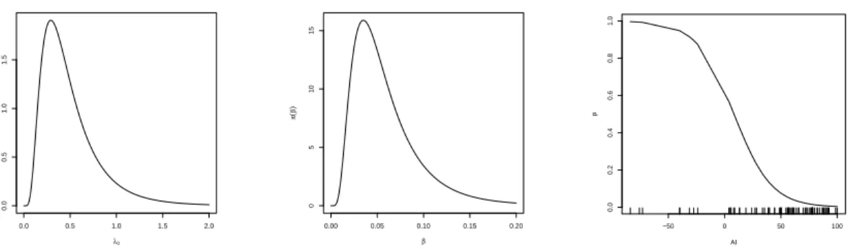
Suppose that for each area is available a set of covariates Xi = (Xi1, ..., Xik)

re-lated to, for instance, the socioeconomic/educational level or access to health services, which provide information on suspect regions of underreporting. Such covariates might be used to appropriately model the uncertainty about the underreporting probabilities

p = (p1, ..., pn). A priori, it is expected that regions with the worst social deprivation

indicators have pi close to 1.0 whereas regions with the best ones have pi close to 0.0.

(43)

Xj, j = 1, ..., k, such that the underreporting probability pi can be modeled using a

logit regression model given by

log

pi

1−pi

= logit(pi) =λ0+βXi, (3.4)

whereβ = (β1, ..., βk) and the prior distributions of eachβj, j= 1, ..., kmust put positive

probability mass in the appropriate part of the real axis R (positive or negative part) depending on the ordering of the associated covariate Xj. If the highest values for the

social deprivation indicator Xj are associated to the worst regions, then βj must have

domain on the positive real numbers, R+. Similarly, if the highest values for the social deprivation indicator Xj are associated to the best regions, then βj must have domain

on the negative real numbers, _R−_{. By doing that, we ensure the desired relationship} between pand Xj, which should disclose that the highest values for the underreporting

probabilities are associated to the regions with the worst social deprivation indicators. In this context, we propose the following Bayesian hierarchical model

Yi|γi, µi ind

∼ CP(µi)

log µi = log Ei+ log θi

θi ind

∼ πθi

γi|pi ind

∼ Ber(pi)

logit(pi) = λ0+βXi

λ0 ∼ πλ0

β ∼ π_β,

whereθi represents the true relative risk associated to areaiandEi denotes the expected

number of cases in such area. As before, by notation CP(µi) we mean that observation

Yi has a Poisson distribution with rate µi and, given µi and γi, the contribution of this

observation for the likelihood function corresponds to the i-th term of the function in (3.3).

Obviously, several structures can be chosen for modeling the relative risks θi. For

example, in a simple context an appropriate Gamma prior distribution can be assigned for each θi. In other case, random effects may be introduced in the modeling of µi to

account for extra-Poisson variations, so that

(44)

whereυi is a non-spatially structured random effect which usually account for the

depen-dence among the counts Y induced by unmeasured covariates and si represents a

spa-tially structured random effect which account for an explicit spatial dependence among the countsY. Details on this modeling strategy were discussed in Section 2.1.1.

Also, the relative risk θi may be modeled including a suitable linear combination of

available covariates W = (W1, ..., Wl) related to suspected risk factors measured in each

area i, so that

logµi = logEi+ l

X

j=1

ωjWij +υi+si.

From the modeling point of view, both sets of covariates X and W might be equal,

overlapping or one might be a subset of the other (Dvorzak and Wagner, 2015). However, when all available variables are included as regressors in both parts of the model (in the Poisson and logit parts), model identification may require additional information and it must be investigated.

The joint distribution of the complete model is given by

π(Y,γ,θ, λ0,β) = L(µ,γ;Y)π(γ|λ0,β)π(θ)π(λ0)π(β)

=

n

Y

i=1

gi(λ0,β) 1−FYi|µi(yi−1)

γi

(3.5)

× (1−gi(λ0,β))fYi|µi(yi)

1−γi

πθi

o

πλ0πβ,

wherefYi|µiandFYi|µi are as defined in 3.3 andgi(λ0,β) = pi = (1+exp{−(λ0+βXi)}) −1

.

3.2 Posterior Sampling Scheme

A convenient MCMC sampling scheme must be implemented for posterior inference. Such scheme corresponds to the Gibbs Sampler, which is based on the full conditional distribution (fcd) of all parameters and latent random variables involved in the proposed

model. To establish notation, let V be a vector with m components and denote by

V−i the vector V without thei-th component, that is, V−i = (V1, ..., Vi−1, Vi+1, ..., Vm).

Define ψ = (θ, λ0,β). Assuming the joint distribution in (3.5), we obtain the fcd of all quantities involved in the proposed model.

For i= 1, ..., n, the full conditional distribution of θi is given by

π(θi|Y,γ,ψ−θi) ∝

fYi|µi(yi)

1−γi

1−FYi|µi(yi−1)

γi

(45)

Therefore, if a Gamma(αi, φi) prior distribution is assigned to the relative riskθi, its fcd

assumes the following different expressions depending if areaiis censored or non-censored

π(θi|Y,Z,γ,ψ−θi) ∝

(

Gammayi+αi,_E_i_φφ_ii+1

, if γi = 0,

Gamma (αi, φi)×

1−FYi|µi(yi−1)

, if γi = 1.

(3.6)

For the i-th component of the latent censoring vector γ the fcd has closed form and it is given by

π(γi|Y,γ−i,ψ) ∝ L(Yi|θi, γi)π(γi|λ0,β) (3.7)

∝ gi(λ0,β)

1−FYi|µi(yi−1)

γi

[1−gi(λ0,β)]fYi|µi(yi) 1−γi

therefore, γi|Y,γ−i,ψ ∼ Ber

Ai

Ai+Bi

, where Ai = gi(λ0,β)

1−FYi|µi(yi−1)

and

Bi = [1−gi(λ0,β)]fYi|µi(yi).

The full conditional distribution for β is given by

π(β|Y,γ,ψ₋_β)∝

n

Y

i=1

π(γi|λ0,β)π_β, (3.8)

and the fcd of the parameter λ0 it is similar to (3.8), replacing π_β for πλ0.

Note from (3.5) that the joint distribution of the proposed model involves a cumulative probability function for the censored (underreported) areas and this makes it difficult the posterior sampling process of θ and γ. Particularly, for the posterior sampling of

θ one Metropolis-Hastings step will be needed. However, a worse problem arises in

the posterior sampling process of γ. Note that the fcd of γi in (3.7) involves a direct

comparison between the termsAi andBi. The fact is that termAiis always much higher

than the term Bi, providing a ratio _A_iA+iBi with value always next to 1.0 and, thereby, we generate more censored areas than we should. That problem happens because the term Ai involves a cumulative probability function, whereas the term Bi involves the

probability in a single point.