Instituto do Cérebro
Programa de pós-graduação em neurociências
The influence of interhemispheric connections on
ongoing and evoked orientation preference maps and
spiking activity in the cat primary visual cortex
Tiago Siebert Altavini
Programa de pós-graduação em neurociências
The influence of interhemispheric
connections on ongoing and evoked orientation
preference maps and spiking activity in the cat
primary visual cortex
Tiago Siebert Altavini
Programa de pós-graduação em neurociências
The influence of interhemispheric
connections on ongoing and evoked orientation
preference maps and spiking activity in the cat
primary visual cortex
Tese apresentada ao Programa de Pós-graduação em neurociências da Universidade Federal do Rio Grande do Norte como requisito parcial à obtenção do Título de Doutor em Neurociências
Tiago Siebert Altavini
Advisor: Kerstin E. Schmidt
Tiago Siebert Altavini
The influence of interhemispheric
connections on ongoing and evoked orientation
preference maps and spiking activity in the cat
primary visual cortex
Tese apresentada ao Programa de Pós-graduação em neurociências da Universidade Federal do Rio Grande do Norte como requisito parcial à obtenção do Título de Doutor em Neurociências
Aprovada em 29 de janeiro de 2016
Banca Examinadora
Prof.ª Dr.ª Kerstin Erika. Schmidt (Presidente)
Universidade Federal do Rio Grande do Norte
Prof.º Dr.º Adriano Bretanha Lopes Tort
Universidade Federal do Rio Grande do Norte
Prof.º Dr.º Sergio Tulio Neuenschwander Maciel
Universidade Federal do Rio Grande do Norte
Prof.º Dr.º Bruss Rebouças Coelho Lima
Universidade Federal do Rio de Janeiro
Prof.º Dr.º Jerome Paul Armand Laurent Baron
Agradecimentos
À Kerstin por ter me recebido em seu laboratório e ter confiado em mim. Agradeço pela orientação sempre presente, pela paciência com minhas limitações e pelo tratamento, sempre horizontal e amigável e pelo exemplo de dedicação no trabalho.
Ao Sérgio Neuenschwander pelo sistema de aquisição de dados em eletrofisiologia e disposição em nos auxiliar durante os experimentos.
Ao David Eriksson e Thomas Wunderle, que nos ajudaram a montar e colocar o laboratório em funcionamento.
Aos amigos por todo o apoio, especialmente nos momentos de dificuldades, técnicas ou pessoais. Agradeço especialmente ao Fábio Caixeta, que me convenceu a vir à Natal e fazer parte deste instituto, e ao Sérgio Conde, que, além do apoio pessoal, nunca cobrou nada pelas aulas particulares de Matlab®.
Á toda equipe que cuida dos sujeitos experimentais. O trabalho de vocês tornou o meu mais fácil.
À minha família, pela total liberdade e apoio que sempre foram dados em todas as minhas escolhas profissionais.
Resumo
No córtex visual primário neurônios com características fisiológicas semelhantes estão agrupados em colunas ao longo das seis camadas corticais. Estas colunas formam os mapas modulares de orientação. Fibras horizontais de longo alcance estão associadas à estrutura destes mapas, uma vez que elas não conectam as colunas de forma aleatória; elas se agrupam em intervalos regulares e interconectam predominantemente colunas de neurônios que respondem a estímulos com características semelhantes. Mapas de orientação preferencial – a ativação conjunta de domínios que preferem a mesma orientação – podem emergir de forma espontânea a já foi especulado que padrões estruturados de atividade espontânea poderiam ser causados pela conectividade irregular, em “manchas”, subjacente do córtex visual. Sabendo que conexões horizontais de longo alcance compartilham muitas características, e.g. agrupamento, seletividade de orientação, com conexões visuais inter-hemisféricas (VIC) pelo corpo caloso nós utilizamos as últimas como um modelo para conectividade lateral de longo alcance.
Para abordar a questão da contribuição da conectividade lateral na geração de mapas espontâneos em um hemisfério nós investigamos como estes mapas reagem à desativação das VIC originadas no hemisfério contralateral. Com este objetivo realizamos experimentos em oito gatos adultos.
Registramos imagens por meio de pigmentos sensíveis a alteração de potencial elétrico (VSD) e a atividade eletrofisiológica de potencias de ação em um hemisfério cerebral enquanto desativamos as VIC de forma reversível no hemisfério contralateral com uma técnica de resfriamento. Com o intuito de comparar o efeito da desativação na atividade evocada ao efeito na atividade espontânea apresentamos como estímulo visual uma série de grades. As grades possuíam oito diferentes orientações distribuídas igualmente entre 0º e 180º. Os quadros isolados de imagens obtidos foram então comparados a mapas de orientação obtidos pela média de várias apresentações do estímulo. Essa comparação foi feita em diferentes situações: basal, resfriamento e recuperação. Mapas auto-organizáveis de Kohonen também foram utilizados como uma forma de análise sem suposição prévia de padrões da atividade espontânea (como os mapas de orientação obtidos pela média de várias apresentações). Também avaliamos se o resfriamento causou efeito diferencial entre a atividade de potenciais de ação evocada e espontânea em unidades neuronais individuais.
atividade espontânea, mas não na atividade evocada. O mesmo resultado foi alcançado ao treinar mapas auto-organizáveis com os dados obtidos por registro de imagens. Os potenciais de ação de unidades com preferência cardinal também decresceram em frequência significativamente mais na atividade espontânea que na evocada.
Baseados nestes resultados chegamos as seguintes conclusões:
1) VIC não são um fator determinante para a estrutura dos mapas espontâneos. Os mapas continuam a ser gerados espontaneamente com a mesma qualidade, provavelmente por uma combinação da atividade espontânea de redes recorrentes locais, do laço tálamo-cortical e de conexões de retroalimentação.
2) VIC são responsáveis por um viés cardinal de probabilidade na atividade espontânea, i.e. ao desativar VIC a probabilidade de um mapa cardinal surgir espontaneamente diminui.
Abstract
In the primary visual cortex, neurons with similar physiological features are clustered together in columns extending through all six cortical layers. These columns form modular orientation preference maps. Long-range lateral fibers are associated to the structure of orientation maps since they do not connect columns randomly; they rather cluster in regular intervals and interconnect predominantly columns of neurons responding to similar stimulus features. Single orientation preference maps – the joint activation of domains preferring the same orientation - were observed to emerge spontaneously and it was speculated whether this structured ongoing activation could be caused by the underlying patchy lateral connectivity. Since long-range lateral connections share many features, i.e. clustering, orientation selectivity, with visual inter-hemispheric connections (VIC) through the corpuscallosum we used the latter as a model for long-range lateral connectivity.
In order to address the question of how the lateral connectivity contributes to spontaneously generated maps of one hemisphere we investigated how these maps react to the deactivation of VICs originating from the contralateral hemisphere. To this end, we performed experiments in eight adult cats.
We recorded voltage-sensitive dye (VSD) imaging and electrophysiological spiking activity in one brain hemisphere while reversible deactivating the other hemisphere with a cooling technique. In order to compare ongoing activity with evoked activity patterns we first presented oriented gratings as visual stimuli. Gratings had 8 different orientations distributed equally between 0º and 180º. VSD imaged frames obtained during ongoing activity conditions were then compared to the averaged evoked single orientation maps in three different states: baseline, cooling and recovery. Kohonen self-organizing maps were also used as a means of analysis without prior assumption (like the averaged single condition maps) on ongoing activity. We also evaluated if cooling had a differential effect on evoked and ongoing spiking activity of single units.
We found that deactivating VICs caused no spatial disruption on the structure of either evoked or ongoing activity maps. The frequency with which a cardinally preferring (0º or 90º) map would emerge, however, decreased significantly for ongoing but not for evoked activity. The same result was found by training self-organizing maps with recorded data as input. Spiking activity of cardinally preferring units also decreased significantly for ongoing when compared to evoked activity.
1) VICs are not a determinant factor of ongoing map structure. Maps continued to be spontaneously generated with the same quality, probably by a combination of ongoing activity from local recurrent connections, thalamocortical loop and feedback connections.
2) VICs account for a cardinal bias in the temporal sequence of ongoing activity patterns, i.e. deactivating VIC decreases the probability of cardinal maps to emerge spontaneously
Summary
1. Introduction ... 1
1.1. Visual system ... 1
1.1.1. Cortical Receptive fields ... 2
1.1.2. Long-range lateral connections ... 2
1.1.3. Visual Interhemispherical Connections ... 5
1.2. Ongoing activity... 5
2. Objectives ... 6
3. Material and Methods ... 8
3.1. Surgical Procedures ... 8
3.2. Reversible Deactivation by Cooling ... 8
3.3. Visual Stimulation ... 10
3.4. Recording Procedures ... 11
3.4.1. Imaging... 11
3.4.2 Electrophysiology ... 11
3.5. Data Analysis ... 12
3.5.1. Kohonen self-organizing maps... 15
3.5.2. Spiking activity analysis ... 16
3.5.3. Upstate windows ... 17
3.5.4. Modulation Index ... 17
4. Results ... 18
4.1. Ongoing modular maps continue to be generated during deactivation of interhemispheric input ... 18
4.2. Absence of interhemipsheric input lowers the frequency of spontaneous but not evoked cortical maps with cardinal preference ... 19
4.3. Evoked and ongoing maps training a Kohonen model ... 23
4.4. Effects of VIC input on evoked and ongoing spiking activity depend on the absolute orientation preference ... 24
5. Discussion ... 28
5.1. Methodological considerations ... 29
5.2. Interhemispheric input does not generate ongoing modular maps ... 29
5.3. Cardinal bias: a quick review ... 31
5.3.1. Lateral connections account for a cardinal bias in ongoing activity 33 5.4. Anisotropy between networks linking neurons preferring horizontal, vertical or oblique contours ... 33
1 1. Introduction
The neurological processes that allow us to perceive the environment have been widely studied throughout neuroscience history. Among all senses, vision is the one we know most about. The knowledge we have about the visual system today allows us not only to grasp the understanding on how we see things but also to predict and test general rules on how neurons function, connect with each other and give rise to large and complex networks throughout the brain.
1.1. Visual system
Simply put, the visual system is composed of: 1) the retina within the eye 2) the lateral geniculate nucleus (LGN) within the thalamus and 3) different cortical areas within the occipital lobe. In the retina, we find the photoreceptors, responsible for the transduction of light into an electric signal. Photoreceptors are connected to bipolar cells, which connect to retinal ganglion cells. Bipolar cells transmit a graded postsynaptic potential to ganglion cells that in turn generate action potentials to be transmitted to the LGN via the optic nerve.
Before reaching the LGN, fibers originating from the nasal hemiretina cross at the optical chiasm while fibers originating from the temporal hemiretina remain ipsilateral. This way, the LGN receives input from both eyes. Ipsilateral fibers contact LGN layers 1 (A), 4 (C) and 6 (C2) while contralateral fibers contact layers 2 (A1), 3 (C1) and 5. From the LGN, neurons project to the primary visual cortex.
Particularly in cats, Brodmann areas 17 and 18 both receive direct input from the LGN and therefore both can be considered primary visual areas. In terms of anatomy, visual field representations and corticocortical connections, these areas can be considered homologues to areas V1 and V2 in macaque (Payne, 1993). Afferent fibers from the LGN reach layer IV of both areas, though area 17 receives input from both the X- and Y-System while area 18 is dominated by the Y-System. X- and Y-Systems are defined on anatomical and functional differences of retinal ganglion cells. In the cortex, this organization accounts for the fact that area 17 neurons are more sensitive to high spatial and low temporal frequencies and have small receptive fields while area 18 neurons are more sensitive to low spatial and high temporal frequencies with large receptive fields.
2 1.1.1. Cortical Receptive fields
Neurons in the LGN and the retina have concentric receptive fields with
center/surround antagonism. These neurons respond better to light spots in the “on” region and either do not respond or are inhibited by stimulation in the “off” region.
Neurons in primary visual cortex respond to slightly more complex stimuli than LGN and retinal neurons. They present elongated receptive fields and respond well to bars and gratings in certain orientations (orientation selectivity). Orientations other than the preferred one will elicit less spiking activity and might even cause inhibition when they are orthogonal to the preferred orientation. Based on their receptive field properties, neurons in the primary visual cortex can be divided into simple and complex cells (Hubel and Wiesel, 1962). Simple cells respond to static and moving bars of the preferred orientation and their receptive fields exhibit clear “on” and “off” regions.
Complex cell receptive fields do not have clearly distinguishable “on” and “off” regions
and respond primarily to bars moving in certain directions (direction selectivity).
A feed forward model initially explained the properties of primary visual cortex receptive fields. This model predicted that LGN neurons arranged along a certain axis project their axons onto the same cortical neuron, giving rise to the elongated and oriented cortical receptive field (Hubel and Wiesel, 1962). However, input from other parts of the same cortical area, from other areas and even from the other hemisphere might contribute to shape the response of a primary visual cortex neuron to a stimulus presented inside its receptive field. (Allman et al., 1985; Angelucci and Bressloff, 2006). In fact, in layer IV of areas 17 and 18, where feedforward LGN fibers connect to the cortex, only 5% to 10% of excitatory synapses come from the LGN (Peters and Payne, 1993; Ahmed et al., 1994).
1.1.2. Long-range lateral connections
3 Orientation preference columns have an organization pattern around
singularities, also called “pinwheel centers”. These singularities are frequently localized on peaks of ocular dominance (Crair et al., 1997; Hübener et al., 1997). If we draw a 100 µm circle around this pinwheel centers we will find orientation preferences of all angles in a continuous manner. In a straight line on the cortex surface it usually takes 750 µm to go through all orientations (Hubel and Wiesel, 1962).
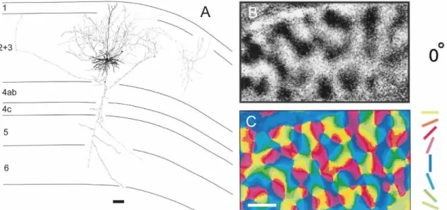
Figure 1.1. A: Reconstruction from a pyramidal layer 3 neuron. Note the dense local axon ramifications (scale bar = 100 µm, modified from Gilbert and Wiesel 1983). B: Intrinsic signal imaging with horizontal bar stimulation. Dark patches are large populations of neurons preferring horizontal stimuli. C: A color coded image constructed from a series of black and white images like B, allowing us to identify all orientation preferences in a single orientation map (scale bar = 1 mm, modified from Hübener et al 1997).
4
the structure of maps acquired through visual stimulation has been suggested (Muir et al., 2011). The synapses are mostly excitatory, with only about 5% to 20% of the synaptic boutons targeting inhibitory cells (LeVay, 1988; McGuire et al., 1991). Finally, it is important to note that long-range connections might account for the majority of excitatory synapses present in a column (Boucsein et al., 2011). The proportion of projections from outside the column making synaptic contact to a cat primary visual cortex neuron can reach values as high as 92% (Stepanyants et al., 2009).
Besides evidence that distant neurons with similar orientation preference can be activated coherently (Ts’o et al., 1986; Hata et al., 1991), studies combining electrophysiological recordings and tracer injections show a higher probability of long-range axons ending close to neurons with the same orientation preference as the origin of that axon (Malach et al., 1993; Bosking et al., 1997; Schmidt et al., 1997b; Sincich and Blasdel, 2001). Such correlation was not found in animals without columnar organization (Van Hooser, 2007). These orientation selective lateral connections may have an important role integrating information from the extra-classical visual surround
by modulating the “classical” receptive field response. A collaboration of columns can
also create a long receptive field, necessary for the recognition of large objects (Bolz and Gilbert, 1989). Visual “pop-out”, collinear facilitation or perceptual grouping could
also rely on this lateral balance of activation (Bosking et al., 1997; Schmidt et al., 1997a), as well as identification of stimuli from noisy background (Field et al., 1993; Kapadia et al., 1995) and multiple simultaneously appearing objects (Boucsein et al., 2011).
5 1.1.3. Visual Interhemispherical Connections
The visual cortex of each hemisphere only processes information of the contralateral visual hemifield, i.e. the right visual cortex processes information from the left visual hemifield and vice versa. In order to maintain a perceptual continuity the two visual cortices need to be extensively connected, which happens through the corpus callosum. With this in mind, it is easy to imagine that visual interhemispheric connections (VIC) have a similar function as the lateral connections introduced in the last section. In fact, it was determined quite early that central parts of the visual field are represented in callosal connections (Choudhury et al., 1965; Hubel and Wiesel, 1967; Berlucchi and Rizzolatti, 1968).
It is still unclear if VIC have unique features or are similar enough to long-range connections so that we can think of VIC between the early visual areas merely as a perpetuation of the intrahemispheric network across the visual field’s vertical midline (Schmidt, 2013). There is, however, growing evidence for the latter. VIC share many anatomical features with long-range lateral connections. Both connections form patchy axonal arbors similar in size and shape (Kisvarday and Eysel, 1992; Houzel et al., 1994; Houzel and Milleret, 1999) and link cells with similar orientation preference (Schmidt et al., 1997b; Rochefort et al., 2009) and with receptive fields aligned along the same axis (Schmidt et al., 1997a). Given these similarities, we chose VIC as a model for long-range lateral connections. VIC presents a good alternative for causal investigations of lateral connections since we are able to manipulate one hemisphere and record brain activity on the other, avoiding that the manipulation itself interferes with our data.
1.2. Ongoing activity
6
output such as perception or behavior (Fiser et al., 2004). Therefore, the study of ongoing brain activity may reveal network features that stimulation cannot.
We already know that ongoing brain activity is not random. It has spatial features resembling neural ensembles co-activated by stimulation or task performance. In visual cortex, spontaneous neuronal firing is strongly correlated between functionally related neurons (Tsodyks et al., 1999). Evoked spiking patterns for specific sound frequencies seem to replay from a wider set of possible spontaneous patterns (Luczak et al., 2009). Spontaneous activation of a large population of neurons is capable to generate modular maps of iso-orientation preference in the primary visual cortex (Kenet et al., 2003). Even larger networks of ongoing activity between cortical areas, resembling evoked activity have been observed (Smith et al., 2009). These networks are often referred to as intrinsic connectivity networks (ICNs) or resting-state networks (RSNs) (Sadaghiani and Kleinschmidt, 2013).
2. Objectives
When deactivating the primary visual cortex of one hemisphere, there is an average decrease of firing rate in the receiving hemisphere. This decrease is stronger when the direction of movement of the visual stimulus points from the deactivated towards the recorded visual hemifield than the other way around (Peiker et al., 2013). Peiker et al (2013) also demonstrated that, before stimulus presentation, ongoing firing rates of neurons preferring this motion direction decrease more than for neurons preferring the recorded-deactivated hemifield direction. These findings reinforce both the ideas of VIC as extensions of the lateral network and ongoing activity functioning as a forecaster of possible visual stimulus trajectories.
7
activity of a single neuron can be predicted by the spatial pattern of ongoing population activity in a large cortical area (Tsodyks et al., 1999) we also examined spiking activity during these conditions.
We anticipated the following possible outcomes from our experiments: During deactivation of VIC
ongoing patterns resembling structured evoked activity become destroyed and thus statistically insignificant, i.e. undistinguishable from random neural activity.
ongoing patterns remain unaltered, exhibiting no difference to ongoing patterns observed with intact VIC.
ongoing activity undergoes some modifications in its spatial and/or temporal features but is still statistically significantly structured. Its features become distinct from both ongoing patterns observed with intact VIC as well as random neural activity. Such modifications could be:
o The similarity between ongoing and evoked activity
decreases/increases.
o Ongoing maps significantly spatially correlated with evoked maps
are generated with lower probability.
o The cardinal bias in ongoing activity becomes weaker/stronger.
8 3. Material and Methods
3.1. Surgical Procedures
Eight adult cats, five males and three females, received a craniotomy on both hemispheres covering a portion of both areas 17 and 18 as well as the 17/18 border region. For surgery, animals were initially anesthetized with an intramuscular injection of ketamine (10mg/kg) and xylazine (1mg/kg) supplemented with atropine (0.1mg/kg). Anesthesia was maintained after tracheotomy by artificial ventilation with a mixture of 0.6/1.1 % halothane (for recording/surgery, respectively) and N2O/O2 (70/30%). After surgery each animal was paralyzed by a bolus injection of 1mg pancuronium bromide followed by continuous intravenous infusion (0.15mg/kg/h).
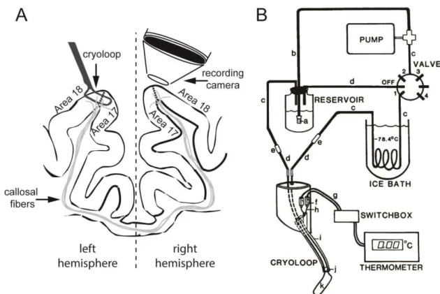
Over the left craniotomy, a recording chamber was implanted, fixed with dental cement and, after removal of the dura mater, filled with silicon oil for intrinsic signal and voltage-sensitive dye (VSD) imaging. In case of VSD imaging, the cortex was first stained with a commercially available blue dye (RH 1838, Optical Imaging Inc) and then covered with silicon oil. Over the right hemisphere, a surface cryoloop (Lomber et al., 1999) was placed and covered with clear agar (Figure 3.1A). All procedures were performed in accordance with the guidelines of the Society for Neuroscience and the university ethics committee for the use of animals (CEUA-UFRN).
3.2. Reversible Deactivation by Cooling
A common research approach in systems neuroscience is the manipulation of certain neuronal connections to evaluate how these connections affect well known brain activity patterns. The main advantage of this approach is that it may establish causation between a neuronal network and a certain pattern, and not just correlation. This is the approach we use in this work, where orientation maps are our pattern, VIC our connections and reversible deactivation by cooling our manipulation.
Neuronal deactivation by cooling consists of lowering neurons’ temperature until action potentials become absent. Most neurons will cease measurable electrical activity at 20ºC. This process is reversible and once neurons reach normal body temperature (between 2-3 min after cooling is turned off) their spiking activity returns with no impairment (Lomber et al., 1999).
We used a reversible deactivation mechanism similar to the one described by Lomber et al (1999). The cooling probes were made of hypodermic stainless steel
9
The methanol was chilled by dry ice to -65ºC. As the methanol tends to rewarm once it leaves the ice bath, the temperature of the cooled cortical surface was regulated by the speed of the pump. A thermometer connected to a sub-miniature connector, attached to a copper wire soldered to the union of the loop was used for temperature monitoring. We kept the cooling probe temperature around 1ºC. The cooling spread at this temperature is expected to be around 1.5-2.5 mm around the probe. The tissue should be around 5ºC in this case and therefore no damage to the tissue is expected. Considering the cooling spread on brain tissue, the critical temperature to cease activity and the cryoloop dimensions our estimation of the deactivated area is around 10 x 5 mm² (Lomber et al., 1999).
Figure 3.1. Experimental setup. A: position of the cryoloop for reversible deactivation and contralateral recording. B: circuit flushed by chilled methanol, from the reservoir through the pump and then through the ice bath to the cryoloop and back into the reservoir (Lomber et al. 1999).
10 orientation maps. Still, these two subjects were included in electrophysiological analysis.
3.3. Visual Stimulation
Visual stimuli were presented randomly on a 21'' monitor placed 57 cm in front of the cats’ eyes. We used intrinsic signal imaging in order to identify the 17/18 border. To this end, gratings of four different orientations in 45 degree steps and a spatial frequency of 0.5 cyc/deg (for area 17) or 0.1 cyc/deg (for area 18) and a temporal frequency of 2 Hz were moved back and forth for 3000 ms. For VSD imaging, the stimulus set consisted of 12 conditions; two conditions presented a random rapid sequence of static whole-field gratings at 8 different orientations in 22.5 degree steps (0.1 cyc/deg, 2 Hz) each lasting 250 ms, eight conditions presented only one of the eight orientations for 250 ms followed by 3750 ms of dark screen, and two conditions of 4000 ms presenting a dark screen (used for ongoing activity recording). In a similar second stimulus set, stimulus presentations were prolonged to 500 ms each. Stimulus conditions were presented in pseudo-randomized order. In each trial, the recording began 500 ms before the presentation of the stimulus, totaling 4500 ms of recording for all trials. After recording of intrinsic signal and VSD baseline imaging the cryoloop was cooled and, 5 min after reaching a stable temperature, VSD imaging was repeated. Cooling would then be switched off and we would wait at least 20 min before a new VSD imaging. We refer to each of these recording sessions as baseline, cooling and recovery. In order to keep non-cooling related signal decay within one session small, each stimulus condition was repeated only 5 times in one session, with 25 s of inter-stimulus interval (ISI), adding to about 30 minutes imaging time per session. For one staining we normally ran three repetitions of the cycle baseline–cooling-recovery, and we stained twice per animal. Only one staining, the one with the most evident orientation maps, was considered for analysis.
For electrophysiology, we determined beforehand receptive field position, extent, orientation and direction preference of all recorded units by presenting whole-field bars moving in 16 different directions (22.5° steps) at a width of 1° and a speed of 20 degrees/s for 2000 ms as in Botelho et al. (2012). The test stimuli for cooling were the same as for VSD imaging, but with an ISI of 2 s and 20 repetitions for each condition.
11
3.4. Recording Procedures
3.4.1. Imaging
Image frames were acquired with a 12mm CCD camera (Dalsa 1M60) through a macroscope fitted with a 1x objective (Imager 3001, Optical Imaging Inc, New York, USA). Intrinsic signal imaging was used only to define the transition zone (TZ) between areas 17 and 18. Two sets of gratings with different spatial and temporal frequencies were presented for an optimal response of either area 17 or 18. The subtraction of the signal obtained by presentation of these two sets made the transition zone between the two areas evident. Rate of acquisition was 5Hz and resolution 512 x 512 pixels.
After intrinsic signal imaging we performed VSD imaging. The first step in VSD imaging is to stain the brain with the dye. For each subject we dissolved 0.8 mg of RH-1838 blue dye in a 1.5 ml buffer solution, which was sufficient for two stainings. The dye was let in contact with the brain for two hours and then the excess removed. The recording chamber would then be filled with silicon oil and sealed, always avoiding the presence of air bubbles inside the chamber. The camera was positioned above the recording chamber (Figure 3.1A) and the focus set slightly below cortical surface (around 200 µm below). Camera recording settings were changed to 160 Hz and 256 x 256 pixels of time and space resolution.
The dye molecules, bound to the neuronal membrane, suffer conformational changes when the membrane potential changes. This change in conformation results in a change of spectral properties and the amount of light the dye reflects or absorbs varies to the degree of membrane potential change. This change in reflectance is detected as an increase in brightness. So, highly activated areas on the cortex are visualized as brighter while lowly activated or inhibited areas are darker (Grinvald and Hildesheim, 2004).
3.4.2 Electrophysiology
For electrophysiology recordings, 4x4 Tungsten microelectrode arrays (1MΩ, 50
12
most of our recorded units had their RF in the contralateral field. Electrodes were lowered between 200-600 µm below cortical surface using a Microdrive (Narishige, Tokyo, Japan) and subsequently, the craniotomy covered with agar. Recorded signals were amplified (1000-fold), band-pass filtered (0.7-6 kHz), digitized, and thresholded around 4 standard deviations above noise level to obtain spike time stamps and spike-wave forms using a Plexon acquisition system (Plexon Inc., Dallas, TX) and custom written Acquisition software (SPASS by Sergio Neuenschwander, in LabView, National Instruments).
3.5. Data Analysis
All analyses were performed in Matlab (Mathworks Inc., Natick, MA, USA). VSD imaging data were subjected to a noise removal procedure in order to make the signal more evident. To this end, we subtracted the first stimulated frame from the whole 4.5 s recording on the single trial level (first frame correction). Secondly, we removed the heartbeat and respiration artifacts from the signal. Two strategies were used to extract heartbeat noise, one for the stimulation set of 250 ms gratings and another for the set of 500 ms gratings. In the first case, a reject band filter covering frequencies between 2.5 and 3.5 Hz was applied (the heart frequency usually remained between 150 and 200 beats/minute). In the latter case, a band pass filter isolated the signal between 2.8 and 3.4 Hz, which was then subtracted from the original signal. The reason for two sets of stimuli and two filtering procedures is the heart frequency variation between subjects. The 2.5-3.5 Hz reject band filter and the 250 ms stimulation were not as effective in producing a quality signal for subjects with a high frequency heart beat (>180 beats/minute) as the 500 ms stimulation combined to the 2.8-3.4 Hz subtraction. In both cases a Discrete Wavelet Transform was applied to remove respiration noise. Considering that the camera has a sample rate of 160 Hz, we were able to remove frequencies between 0 and 0.625 Hz (respiration was never faster than 0.3 Hz) at the seventh decomposition level.
13
Subsequently, regions of interest (ROIs) - areas of cortex void of blood vessels and responsive to the stimuli – were selected from the maps (Figure 3.2). Based on these ROIs we then calculated the spatial Pearson correlation coefficient of frames acquired through grating stimulation or ongoing frames with the averaged single condition maps. This resulted in eight correlation values for each frame, evoked or ongoing. All analyses were done separately for baseline, cooling and recovery recordings.
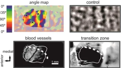
Figure 3.2. . Top-left: angle map with all orientation preferences displayed, the shaded region is outside the ROI. Arrowheads point to pinwheel centers. Top-right displays an artificially generated map from control 2. Bottom-left: surface image of blood vessels from the recorded area. Bottom right: difference image obtained by intrinsic signal imaging with two different spatial frequencies (0.1.cyc/deg, 16 deg/sec and 0.5 cyc/deg, 4 deg/sec) in order to identify the 17/18 border. Dark region, area 18; lighter modulated region, area 17. White continuous line, analyzed region-of-interest (ROI); white dotted line, approximate 17/18 border from difference imaging. Note that both evoked and ongoing map layouts are widely preserved during VIC deactivation.
Since single trials, and especially single frames, may contain a lot of noise (activity not related to stimulation or patterned activity waves), erroneously indicating structure, we calculated the vector sum of all eight raw correlation coefficients produced by each frame when correlated with each of the eight single orientation maps. These coefficients were disposed in a circle (with correlation coefficients calculated from orthogonal maps in opposite directions) and the resultant vector was calculated (Fig 3.3). To calculate the angle of the resultant vector we must first calculate two components a and b:
= ∑ � cos
�−
14
= ∑ � sin
�−
=
Where � is the correlation coefficient obtained for a set N of stimulus orientations , � = , … − , which are uniformly distributed over 0º-180º. In electrophysiology � is the firing rate for a certain stimulus orientation. The angle of the resultant vector, θ, can then be calculated as:
� = .5 tan− � >
or
� = 8 + .5 tan− � <
The resultant vector angle θ defines which map structure the frame mostly resembles. We can then use the vector magnitude (referred to as tuning index) to define how well it matched the respective single orientation map. The tuning index (TI) was calculated as:
�� = + /
15
Figure 3.3. A frame correlation coefficient vectors to the single condition orientation map generated by each oriented grating (gray arrows). The black arrow is the vector resultant correlation coefficient vectorial addition.
As a control, we used artificially generated maps of the same size as the original ones but containing pixel values randomly chosen from a uniform distribution between 0 and 1 (control 1). Each of these random maps was submitted to the same filtering process as recorded frames. Another control technique (control 2) was to convolute these artificially generated maps with single condition maps prior to spatial filtering. After the convolution we would make a series of circular shifts in pixel rows and columns in order to obtain a larger number of artificially generated maps. Control 2 technique is similar to what Kenet et al (2003) used and considered to be more
conservative since it imprints single condition maps features to the artificially generated maps. Convolution between two images is defined by:
∗ , = ∑ , − , − ,
, ��
Where g and f are the images, recorded and randomly generated, and (a,b) the
pixel coordinates of images being convoluted (Figure 3.2).
3.5.1. Kohonen self-organizing maps
In order to classify ongoing frames without any prior assumption of their putative structure we applied an algorithm devolving self-organizing maps (Kohonen, 1990).
16 start to become evident in the self-organizing maps. This analysis is useful for two main reasons: 1) we avoid a possible circular logic of selecting over-the-threshold evoked and ongoing frames and then correlating them to single condition maps that were used to define the threshold in the first place. 2) self-organizing maps may reveal a subtle pattern or effect that was present in frames that didn’t achieve the correlation threshold
to single condition maps. The initial network consisted of 100 nodes, organized as a 10 by 10 network, and was trained by either all ongoing or all evoked frames (training input). In order to determine the distance between the nodes within the network we used a hexagonal topology and a Euclidean distance function defined by:
�, = √∑ �, − �, �
=
where Di,jis the distance between nodes i and j, ni.k is the kth element from a total of P
elements of node i. Training was performed with an initial neighborhood of 10 nodes
and 10 steps. Within each training step q, the node N with higher proximity to the input
frame ℱ and its entire neighborhood is modified to resemble the input even more by following the learning rule:
� = � − + � ℱ � − � −
where α is the learning rate set to decreasing values from 1 to 0.01. The neighborhood gets smaller with each training step, until only one node learns from the input. This process was repeated 40 times (i.e. epochs) for each input frame. Finally, we calculated the correlation coefficient and tuning index for each trained node with the single condition maps the same way we did for recorded frames.
3.5.2. Spiking activity analysis
Recorded multi-unit activity was sorted through Waveclus, a spike sorting toolbox
17
while its magnitude the OI. Since neurons in primary visual cortex may have a large variance in firing rate, and, contrary to correlation coefficients spiking responses are always greater or equal to zero, OI was always divided by the sum of all eight firing rate vectors as such:
� = ∑�−+� /
=
where � is the spiking activity obtained for a set N of orientations , � = , … − , which are uniformly distributed over 0º-180º. This kept the OI between 0 and 1. Further analysis included only units with an OI greater or equal to 0.2. We then calculated the mean firing rate of each selected unit in 500 ms time windows after presentation of the static grating with the unit’s preferred orientation and equal windows of ongoing activity recording from the test protocol.
3.5.3. Upstate windows
In order to avoid artifacts in the analysis caused by too low spike rates we chose windows of high level ongoing activity compared to the overall level of ongoing activity. To this end, we established as a threshold the mean firing rate of all baseline trials plus one standard deviation. For every time point detected above threshold, we considered the activity from 100 ms before until 400 ms after that time point, thus defining 500 ms windows of ongoing activity considered for analysis (upstate window). This was done for baseline, cooling and recovery recording with the threshold always calculated on baseline data.
3.5.4. Modulation Index
The deactivation effect was measured by the modulation index (MI) of the measured and computed variables (D), a dimensionless quantity:
��= �� �� ��� �−�+� ���� ����� �; � ∈ {− … . }
A negative MI means that D (correlation probability, firing rate, tuning) decreased
18 4. Results
4.1. Ongoing modular maps continue to be generated during deactivation of interhemispheric input
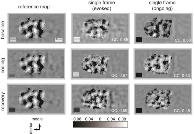
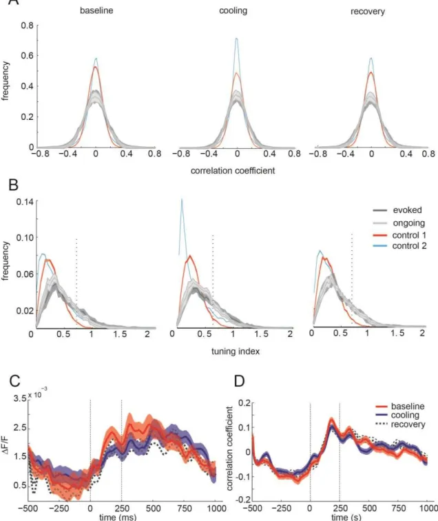
During deactivation of visual interhemispheric connections, the overall layout of the average evoked single orientation map did not change (Figure 4.1, first column). In agreement, during all three states (baseline, cooling, recovery), single evoked frames closely resembling the average map could be traced (Figure 4.1, second column). As Kenet et al. (2003), we detected also frames of ongoing activity modulated in a similar manner as the evoked map. Most interestingly, these spontaneous modulations continued to occur during deactivation of VIC (Figure 4.1, third column) although this procedure removes considerable input from the adjacent half of the visual field representation.
In order to quantify the similarity of single frames with the averaged map we calculated the distribution of all correlation coefficients with the average evoked map for each of the eight orientations and each state. This procedure revealed both high positive and negative correlation coefficients compatible with frames being very similar (positive correlation) to the average columnar pattern evoked by a certain orientation and complementary to the pattern evoked by its orthogonal orientation (negative correlation). Correlations during evoked and ongoing stimulation did not differ significantly from each other during baseline (p = 0.9627), cooling (p = 0.6828) or recovery (p = 0.9926, Kolgomorov-Smirnov two-sample test for all three comparisons, Figure 4.2A, dark grey line, evoked; light gray, ongoing). This suggests that images acquired during ongoing have a clear orientation map pattern.
In order to provide evidence that the structure indicated by high correlation coefficients results from true orientation tuning of the ongoing maps we calculated the vector sum of all eight raw correlation coefficients (Fig. 4.2B). The resultant vector amplitudes (tuning indices) were also not significantly different between evoked and ongoing maps during baseline (p = 0.1181), cooling (p = 0.2865) or recovery (p = 0.1804, Wilcoxon rank sum test for all three comparisons, Figure 3B).
19
(p = 0.00003, Wilcoxon rank sum test, Fig. 4.2D). Figure 4.2C and D combined indicate that, although there is a small signal loss in amplitude, the structure of the maps is fairly maintained.
Figure 4.1. Evoked and ongoing VSD maps. Single frames acquired before (upper row), during (middle row), and after (lower row) reversible cooling deactivation of VIC from the topographically corresponding contralateral transition zone and central area 18. Black and white dotted lines mark corresponding areas on the cortex in all images. CC: correlation coefficient to the reference map.
4.2. Absence of interhemipsheric input lowers the frequency of
spontaneous but not evoked cortical maps with cardinal preference
Kenet et al., (2003) had observed that ongoing frames resembling maps for cardinal orientation preferences were generated with a higher frequency than frames resembling maps for oblique orientation preferences. This is in accordance with earlier observations that in the central visual field representation stimulus-driven responses to cardinal orientations are stronger (e. g. Pettigrew et al. 1968), more frequent (Li et al., 2003) and lead to larger cortical representations of those orientations (e.g. Dragoi et al. 2001).
20
cooling, 31% of evoked recovery, 27% of ongoing baseline, 40% of ongoing cooling and 27% of ongoing recovery frames also exceeded the threshold. These percentages are in reference to a 4000 frames distribution each.
21 in C and D. There was a small decrease in amplitude between 80 and 500 ms after stimulus onset (C) but no significant difference in correlation coefficient values in the same interval (D).
Figure 4.3 demonstrates the probability of a high correlation of single stimulus-evoked frames with an average single condition map for a certain preference angle. Confirming the previous study (Kenet et al., 2003) 68,87% of the evoked (Figure 4.3A) and even more of the ongoing baseline frames (82,84%, Figure 4.3B) were classified as cardinal (either horizontal or vertical) rather than oblique. Interestingly, deactivating VIC did not change this classification for the evoked (68,78% cardinal) activity but decreased the frequency of cardinal frames in ongoing activity to 63,18% as it increased the frequency of oblique classified frames (from 17,74% on baseline to 36,82% during cooling).
Figure 4.3C summarizes the impact of VIC on the angular preference of single frames, expressed as a modulation index (with positive numbers indicating an increase in the frequency for this angular preference during cooling, and vice versa for negative numbers). The changes in the ongoing cardinal bias have little to do with spatial changes in the structure of orientation maps, as results from Figure 4.2 already suggest. Actually, there is a change of probability in time for the appearance of cardinal maps (Figure 4.3D).
For evoked activity (black), the number of frames classified as vertically, obliquely or horizontally preferring maps did not change significantly during cooling. For ongoing activity, the number of frames classified as vertical or horizontal dropped, significantly decreasing the cardinal predominance (* p = 0.002, Wilcoxon signed rank test, 12 datasets), while the number of frames classified as oblique increased also significantly (p = 0.002, Wilcoxon signed rank test, 12 datasets) All distributions recovered to baseline during rewarming.
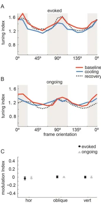
23 Figure 4.4. VSD tuning remains unchanged by VIC deactivation. Average tuning index (y-axis) of single frames at identified preference angles for one dataset during evoked (A) and ongoing (B) recordings. C: Median modulation index (MI) for the tuning magnitude at identified angles for 10 datasets. Dispersions are median absolute deviations. Note the stability of VSD tuning indices during VIC deactivation.
4.3. Evoked and ongoing maps training a Kohonen model
24 correlating recorded frames with average single condition maps (Figure 4.5A). The Kohonen algorithm produced those results also when being fed exclusively with spontaneous baseline data (Figure 4.5B). Unexpected from the previous analysis, the number of evoked frames assigned to horizontal but not vertical orientation preference dropped (Fig. 4.5A). This drop, however - maybe due to a large dispersion in data - was not significant (Fig. 4.5C). One reason for the discrepancy between recorded and trained frame results could be that the bias towards vertical orientations exists and we removed it by restricting the analysis for the actual recorded frames to only those with high tuning indices. Another possibility is that the bias is due to noisy frames entering the Kohonen analysis.
For ongoing templates, the Kohonen analysis reproduced quite closely the result we retrieved from correlation analysis with real data. The number of templates classified as cardinally preferring decreased during VIC deactivation while the number of obliquely preferring frames increased (Fig. 4.5B, C). Both, templates trained with either evoked or ongoing data turned out to be as well tuned as the real data frames. Cooling induced changes in tuning indices as a function of orientation preference were not significant (data not shown).
This confirms that modulated maps resembling the functional architecture of that cortical area continue to be generated frequently and with good selectivity. Only the frequency with which certain orientation preference columns get activated spontaneously changes when part of the lateral network is disrupted.
4.4. Effects of VIC input on evoked and ongoing spiking activity depend on the absolute orientation preference
26
In contrast to the seemingly stable appearance of evoked and ongoing modulated frames in both presence and absence of VIC input, average firing rates decreased significantly during cooling of VIC (14,6 +/- 10,6 % for activity evoked by the preference orientation +/- 30deg, 12,6 +/- 6,55 % for ongoing activity) as has been observed before (Schmidt et al. 2010; Wunderle et al. 2013). In previous work, pre-stimulus activity of neurons driven by contours moving into the cooled hemifield had turned out to be less influenced than that of neurons preferring horizontal contours or such moving out of the cooled hemifield (Peiker et al., 2013). However, there was still missing a systematic comparison with neurons preferring or stimulated by oblique contours as well as with real spontaneous activity long after a stimulus had been presented.
Here, we observed that the exact combination of changes in ongoing and stimulus-derived activity depends on the orientation preference of the neurons under study. Figure 4.6 depicts the average firing rate of three representative example units, one of vertical (A), one of oblique (B), and one of horizontal orientation preference (C). Although there seems to be a change in maximum response latency, the total number of evoked spikes of the unit preferring vertical contours (VN) moving into the cooled hemifield almost does not change during cooling (Figure 4.6A). The same thing can be said for the obliquely preferring unit (Figure 4.6B). Finally, the horizontally preferring unit (HN) presents a prominent spike rate decrease during VIC deactivation (Figure 4.6C). Interestingly, when comparing this picture to the evoked VSD maps it matches the lack of templates assigned by Kohonen learning to horizontal as opposed to vertical orientation preference maps during cooling (Figure 4.5A).
For ongoing activity, however, both VN and HN loose more spikes than the obliquely preferring neurons (Figure 4.6, compare A and C with B). This supports the loss of the cardinal bias in the angular distribution of ongoing maps (Figures 4.3C, 4.5C).
27
28 Figure 4.7. Firing rate changes during VIC deactivation depend on orientation preference. Averaged single-unit activity in the transition zone and central area 18. A: Modulation indices for ongoing activity were significantly lower than those for evoked activity (p = 0.0062, n = 1280 for evoked 469 for ongoing). B: Decrease in activity was significantly greater for ongoing than for evoked activity only for units with cardinal preference (p=0.0271, n = 682 for evoked and 251 for ongoing). C: When separating units according to their orientation preference, it can be observed that horizontally preferring neurons decrease both evoked and ongoing activity. In contrast, vertically preferring neurons decrease predominantly their ongoing rates (p=0.0027 between ongoing and evoked, n = 314 for evoked and 111 for ongoing).
5. Discussion
We have successfully reproduced the findings of Kenet and colleagues (2003). Through visual stimulation and VSD imaging we have established the modular patterns of cortical activation identified as orientation maps and found the same maps in the absence of stimulation. Spiking activity recorded contained units with varying orientation preference and sharpness of tuning. Deactivation of VIC caused significant changes in some features of both imaged and electrophysiological data, but did not change the layout of the maps or the selectivity of the neurons.
29 a higher frequency of ongoing frames being correlated with vertical or horizontal orientation preference maps (Kenet et al., 2003), disappears.
In accordance, ongoing firing rate breakdown is significantly larger for neurons preferring cardinal as opposed to oblique contours. However, neurons preferring horizontal contours (HN) decrease their rates independently of whether being stimulated or not when VICs are deactivated. This is not the case for neurons preferring vertical contours (VN), which exhibit stable rates during visual stimulation but not during resting state.
5.1. Methodological considerations
Since the three sessions – baseline, cooling and recovery – were performed at separate moments, differences between them could be explained by different brain states, with no relation to the cooling manipulation. In order to overcome this constraint, we tried to keep cooling sessions short and repeated them. Since the observed changes were invariable throughout sessions, stainings and subjects, this explanation is unlikely to be true. Still the development of technologies that allow a faster and more precise manipulation of connections, like optogenetics, should be considered for studies following the same paradigm as this. Another limitation of the presented work resides in the cortical area recorded. We only recorded activity from visual area 18 and the TZ between area 17 and 18. However, both areas 18 and 17 of the cat visual cortex can be considered primary visual areas. In order to achieve conclusions about the overall early visual cortical processing, adjustments would have to be made to stimulation and data analysis regarding the preferred spatial and time frequencies of area 17 and repeat experiments with a focus on this particular area. Still, we have no reasons to believe significantly different results would be obtained.
5.2. Interhemispheric input does not generate ongoing modular maps
30
orientation preference maps close to the visual field’s midline representation when
callosal (or feedback) inputs are absent.
More surprisingly, ongoing activity patterns also continue to be generated with the same frequency and tuning. When these ongoing fluctuations were first observed (Kenet et al., 2003) they were attributed to patterned intracortical connections, i.e. patchy long-range lateral axons interconnecting neurons responding to the same feature space, e.g. orientation preference (Gilbert and Wiesel, 1989; Schmidt et al., 1997; Bosking et al., 1997; Malach et al., 1993; Stettler et al., 2002). Accordingly, spontaneous population activity in cortex would be biased toward states that reflect the spatial configuration of that patterned connections (Kenet et al., 2003; Muir et al., 2011).
Given that VIC most likely perpetuate the patchy intracortical network across the hemispheres (Schmidt et al. 1997; Rochefort et al. 2009; Schmidt 2013) we expected to disturb ongoing activity maps close to the densely interconnected 17/18 border when deactivating these inputs. Instead, ongoing fluctuations continue to regularly activate iso-orientation domains. This can have the following reasons.
Firstly, maps are generated by the remaining more local intrinsic network. Models confirm that orientation maps could be generated by indeed local recurrent connections (Somers et al., 1995; Sompolinsky and Shapley, 1997; Ernst et al., 2001; Tao et al., 2006), and intracellular recordings indicate that selectivity arises from the local connectivity context neurons are embedded in (Frégnac et al., 2003). In agreement, the range of functional connectivity – apart from being input-dependent - has been shown to clearly decay with cortical distances larger than 1-1.5 mm (Nauhaus et al., 2009; Chavane et al., 2011).
Secondly, ongoing orientation maps could emerge within the thalamocortical loop. There is evidence that geniculocortical afferents exhibit orientation selectivity at their target structures in layer IV (Chapman et al., 1991). Orientation maps even emerge when lateral connectivity in close vicinity is interrupted during early development (Löwel & Singer 1990). In agreement, orientation selective responses turned out to be quite robust even when cooling cortex in the immediate vicinity of the recorded neuron (Girardin and Martin, 2009).
31 Taken together it is likely that not only the long-range patchy network contributes to the generation of ongoing patterns. Other circuits embedding primary visually cortically neurons into the visual stream, in particular, local and intracortical connections are probably also involved.
5.3. Cardinal bias: a quick review
There is a consistent anisotropic feature in the visual system called oblique effect or cardinal bias. The cardinal bias consists of a series of differences in the cortical representation of oblique versus cardinal orientations. It is derived from studies involving many different paradigms and techniques. Usually subjects have a better performance or a larger cortical representation for stimuli aligned in vertical or horizontal orientations as compared to stimuli in oblique orientations. The cardinal bias is present in the human adult and child and throughout the animal kingdom (Appelle, 1972).
Although the phenomenon of a psychophysical cardinal bias is already well established, its neurobiological origin is still under investigation. The hypothesis that it is generated by the optics of the eye has long been discarded (Campbell et al., 1966; Mitchell et al., 1967) and it is known by now that the cardinal bias is generated in the brain. Several questions were to be addressed. Which cells are involved? How are they
connected? What’s the role of thalamo-cortical, intra-cortical or cortico-cortical connections? What is the influence of feedback?
32 Evidence that tuning sharpness alone was not enough to create a cardinal bias
was soon presented, suggesting that the cardinal bias “anisotropy may result from a predominance in the neuronal population of cells with receptive fields preferentially sensitive to horizontal or vertical foveal targets.” (Mansfield and Ronner, 1978). In fact, a study published in the same year showed that kittens less than three weeks of age have more cells coding for horizontal and vertical orientations regardless of visual experience (Frégnac and Imbert, 1978). There was also a study that failed to find a cardinal bias in either sharpness of tuning or neuronal number (Finlay et al., 1976). Mixed results giving different weight to tuning and neuron population on the cardinal bias rise suggest that the cardinal bias is not a general rule of all primary visual cortex neurons, but a phenomenon found in a network of specific subpopulation of neurons.
Psychophysical studies contribute to this view. Rhesus monkeys have a higher sensitivity for cardinal oriented gratings at high spatial frequency, but not so much at low spatial frequency (Boltz et al., 1979). Humans also have a higher sensitivity to cardinally than obliquely oriented stimuli and this differential sensitivity increases with stimulus length (Orban et al., 1984). Although a cardinal bias in peripheral vision was initially thought to be almost absent, it was described later that it is easier for an observer to accurately judge the angular direction of cardinally oriented gratings, especially for high spatial frequencies (Coletta et al., 1993). Gros and colleagues came to a similar result. They found that, although detection thresholds are invariant to motion direction, direction discrimination thresholds are much higher for oblique directions of motion (Gros et al., 1998). A perceptual cardinal bias also exists for chromatic stimuli, but it is stronger in lower spatial frequencies than for achromatic stimuli (Krebs et al., 2000).
33 (Kenet et al., 2003). These ongoing fluctuations in cat primary visual cortex tend to correlate more with horizontal and vertical than with oblique single condition maps and, based on the literature, authors suggest that intrinsic cortical states are largely determined by intra-cortical activity. Our data establish a causal relation between lateral connections and the cardinal bias present in ongoing fluctuations.
5.3.1. Lateral connections account for a cardinal bias in ongoing activity
Deactivating VIC weakens the cardinal bias and most interestingly, this bias was eliminated from ongoing but not from evoked maps and spikes when deactivating VICs. This is in agreement with previous observations that ongoing or cortical responses to low contrast reveal more influence of lateral connections than responses saturated by high contrast stimulation via feedforward input (Nauhaus et al., 2009). It is possible, that a cardinal dominance in the remaining network activated by the stimulus was sufficient to maintain a rest cardinal bias in evoked activity.
We assume that a true redistribution of probabilities with which certain orientation domains got spontaneously activated took. This is more likely than an improvement or impoverishment of different maps as tuning indices of single frames did not change significantly. If the interrupted network produced spontaneous cardinal maps less often the selective loss of spikes in these domains is also explained as spiking is intrinsically linked to the underlying fluctuations (Arieli et al., 1995; Tsodyks et al., 1999).
Our finding thus indicates that synapses conveyed by long-range lateral connections – at least those passing through the corpus callosum - are more numerous or stronger between neurons preferring horizontal and/or cardinal contours.
5.4. Anisotropy between networks linking neurons preferring
horizontal, vertical or oblique contours
The previous study (Peiker et al., 2013) pointed towards an anisotropy of patchy networks interconnecting HN and VN in the vicinity of the 17/18 border. VN reacted less to VIC removal when driven by a stimulus moving into the cooled hemifield, i.e. expecting movement processed by the intact hemisphere. This anticipatory drive would be delivered by a VN interconnecting circuit supposedly more elongated parallel to the 17/18 border.
34 horizontal contours. However HN lose much more ongoing spikes than obliquely preferring neurons and the difference between evoked and ongoing MI for VN is significant, while the same difference for oblique is not. Also the high likelihood to encounter cardinal but not oblique maps in ongoing activity disappears. It is conceivable that we are looking on two superimposed probabilities. First, there might be a rather local anisotropy among connections between different populations of orientation-selective neurons within this particular part of the visual field representation, caused by the split of the visual field at its midline by the corpus callosum. This anisotropy appears only under visual stimulation because we disrupt the network at this localization unilaterally and present a midline-crossing stimulus. Second, there exists a general bias towards long-range connections between neurons preferring cardinal as opposed to more oblique contours in the overall patchy network, which is not necessarily restricted to the 17/18 border. We eliminate that bias from otherwise unimpaired ongoing maps because we disrupt the long-range network and herewith, spontaneous longer-range waves of activity passing through which instruct the cardinal bias in ongoing activity.
According to a recent modeling study the patchy intrinsic network would provide
“a physical encoding for statistical properties of the modality represented in an area of cortex” (Muir et al., 2011). Indeed, statistical properties of natural scenes as viewed by
cats exhibit a bias for cardinal with prevalence for horizontal contours (Betsch et al. 2004). A bias for cardinal orientations is also found in human natural scenes (Nasr and Tootell, 2012).
Thus, the cortical cardinal bias may be an adaptive result of natural scene properties being implemented into the network of long-range patchy connections. This adaptation can have occurred already during evolution and/or is reinforced by postnatal development when the system is exposed to visual experience (Berkes et al., 2011). The latter hypothesis is based on evidence that long-range instrinsic connections develop in an experience-dependent manner (Löwel & Singer 1990; Schmidt et al. 1997). Similarly, visual input can instruct orientation preference of cortical neurons as it can selectively enhance the dominance of certain populations of orientation selective neurons (Singer et al., 1981; Sengpiel et al., 1999). Along this argumentation, strabismus impairs psychophysical performance (Sireteanu and Singer, 1980) and cortical processing of horizontal image movements (Singer et al., 1979) most likely because it alters visual input created by those movements.
35
5.5. Ongoing patterns may not only reverberate anatomical
connections but also play a role in defining them
The ongoing orientation maps patterns we found in our data are patterns we were specifically looking for. Finding these patterns does not eliminate the possibility of other ongoing patterns being present. Frames below our tuning index threshold are not necessarily random, they could be highly correlated to patterns we did not compare them to.
There might be more to ongoing activity than a repercussion of intrinsic anatomical structures. A body of studies with functional magnetic resonance imaging
(fMRI) suggests that a “Hebbian-like shaping of the cortical connectivity patterns that
occur during daily life may play an important role in their detailed organization.” (Wilf et al., 2015). Networks engaged in a visual learning task show differences in resting state activation which are correlated to the degree of perceptual learning (Lewis et al., 2009). Adaptive changes have been also observed in the resting state network between the hippocampus and a portion of the lateral occipital complex after a task requiring highly subsequent memory (Tambini et al., 2010). Only a single epoch of cortical activation may be sufficient to modify the resting state network following a Hebbian-like rule (Harmelech et al., 2013). Further, it has been shown that changes in resting state are associated with motor skill learning and subsequent structural and functional changes in prefrontal and supplementary-motor areas (Taubert et al., 2011).
Taken together, these studies imply that resting state activity patterns precede and play a role in channeling structural changes of certain brain connections. Wilf and colleagues (2015) suggest that this is why resting state activity in visual areas actually resembles activity driven by natural scenes more than activity evoked by optimal stimulation. However, the attempt to link structural changes to resting state modulation in these studies still lacks causality. Namely, in the latter study, it remains unclear whether the resting state resembles the natural scene driven activation patterns because that is what the actual circuit produces during weakly salient stimulation or because the circuit is adapting to this kind of stimulation.