The influence of visual inter-hemispheric connections on spiking, assembly and LFP activities, and their phase relationship during figure-ground stimulation

(1)

UNIVERSIDADE FEDERAL DO RIO GRANDE DO NORTE

Programa de Pós-Graduação em Neurociências

THE INFLUENCE OF INTERHEMISPHERIC CONNECTIONS ON

SPIKING, ASSEMBLY AND LFP ACTIVITIES, AND THEIR PHASE

RELATIONSHIP DURING FIGURE-GROUND STIMULATION IN

PRIMARY VISUAL CORTEX.

SERGIO ANDRÉS CONDE OCAZIONEZ

Natal, 2014

(2)

Programa de Pós-Graduação em Neurociências

THE INFLUENCE OF INTERHEMISPHERIC CONNECTIONS ON SPIKING,

ASSEMBLY AND LFP ACTIVITIES, AND THEIR PHASE RELATIONSHIP

DURING FIGURE-GROUND STIMULATION IN PRIMARY VISUAL CORTEX.

SERGIO ANDRÉS CONDE OCAZIONEZ

Trabalho apresentado ao programa de Pós-Graduação em Neurociências da Universidade Federal do Rio Grande do Norte como requisito para a obtenção do grau de

DOUTOR EM NEUROSCIÊNCIAS

Aprovada em: 31.03.2014

Banca examinadora:

ADRIANO BRETANHA LOPES TORT

JEAN CHRISTOPHE HOUZEL – UFRJ

JEROME PAUL ARMAND LAURENT BARON – UFMG

KERSTIN ERIKA SCHMIDT

SERGIO TULIO NEUENSCHWANDER MACIEL

(3)

Acknowledgments

This work would be impossible without the enormous support of my entire family. Thank you for always be there!

To Prof. Kerstin Schmidt, thank you for the lessons, patience and for having embraced and care this project as her own.

To Beatriz Couto, thank you for coming into this crazy boat with me.

To all my friends, especially to Vitor Santos and Rodrigo Pavão, thank you for all coffees and beers trying to put the puzzle pieces in their place.

(4)

Summary

Abbreviation List ... 4

Resumo... 5

Abstract ... 7

1. Introduction ... 9

1.1. The Primary Visual Cortex ... 12

1.1.1. Lateral Intrinsic Connections ... 15

1.1.2. Visual Callosal Connections ... 17

1.2. Contextual Stimulation ... 19

2. Working Hypothesis ... 24

3. Objectives ... 25

4. Materials and Methods ... 26

4.1. Anesthesia and Physiological Monitoring ... 26

4.2. Recording Area Identification ... 26

4.3. Electrode Implantation ... 27

4.4. Stimuli ... 28

4.5. Cooling Procedure ... 29

4.6. Data Recording ... 30

4.7. Data Analysis ... 31

4.7.1. Orientation and Direction Tuning of Multiunit Activity ... 31

4.7.2. Firing Rates and Power Spectral Density ... 32

4.7.3. Assembly Detection ... 34

4.7.4. Phase Locking ... 38

5. Results... 41

5.1. Recording Site Characterization ... 41

5.2. Raw Responses ... 44

5.3. Segmentation and Cooling Indices for Firing rates and LFPs ... 48

5.4. Assembly Detection and Characterization ... 53

5.5. Segmentation and Cooling Indices for Assemblies ... 56

5.6. Phase Locking ... 59

(5)

5.6.2. Single Cell and Assembly Phase Locking with Natural Scene Stimulation ... 60

5.7. Coherence Variation during the Deactivation of IHCs ... 63

5.8. Summary of Results ... 66

5.8.1. From Individual Recording Sites ... 66

5.8.2. From Population Level... 67

6. Discussion ... 68

6.1. Methodological discussion ... 68

6.1.1. About Visual Stimulation ... 68

6.1.2. About the cooling technique ... 69

6.2. About Figure-Ground Segmentation ... 70

6.3. About the Influence of Interhemispheric Connections on Raw Responses ... 71

6.4. About the Influence of Interhemispheric Connections on Figure-Ground Segmentation ... 72

6.4.1. Spike rates ... 72

6.4.2. LFP power ... 73

6.4.3. Assemblies and Phase Locking ... 76

7. Summary and Conclusion ... 80

8. Supplementary ... 82

(6)

4

Abbreviation List

CI: Cooling Index

CRF: Classical Receptive Field DI: Direction Index

HG: High Gamma

IHCs: Interhemispheric Connections JRF: Joint Receptive Field

LFP: Local Field Potential LG: Low Gamma

OI: Orientation Index

PSD: Power Spectrum Density RS: Recording Sites

(7)

5

A influência das conexões inter-hemisféricas nas atividades de disparo,

de assembleias e de potencial de campo, e sua relação de fase durante a

estimulação figura-fundo do córtex visual primário.

Resumo

Desde os descobrimentos pioneiros de Hubel e Wiesel acumulou-se uma vasta literatura descrevendo as respostas neuronais do córtex visual primário (V1) a diferentes estímulos visuais. Estes estímulos consistem principalmente em barras em movimento, pontos ou grades, que são úteis para explorar as respostas dentro do campo receptivo clássico (CRF do inglês classical receptive field) a características básicas dos estímulos visuais como a orientação, direção de movimento, contraste, entre outras. Entretanto, nas últimas duas décadas, tornou-se cada vez mais evidente que a atividade de neurônios em V1 pode ser modulada por estímulos fora do CRF. Desta forma, áreas visuais primárias poderiam estar envolvidas em funções visuais mais complexas como, por exemplo, a separação de um objeto ou figura do seu fundo (segregação figura-fundo) e assume-se que as conexões intrínsecas de longo alcance em V1, assim como as conexões de áreas visuais superiores, estão ativamente envolvidas neste processo. Sua possível função foi inferida a partir da análise das variações das respostas induzidas por um estímulo localizado fora do CRF de neurônios individuais. Mesmo sendo muito provável que estas conexões tenham também um impacto tanto na atividade conjunta de neurônios envolvidos no processamento da figura quanto no potencial de campo, estas questões permanecem pouco estudadas.

Visando examinar a modulação do contexto visual nessas atividades, coletamos potenciais de ação e potenciais de campo em paralelo de até 48 eletrodos implantados na área visual primária de gatos anestesiados. Estimulamos com grades compostas e cenas naturais, focando-nos na atividade de neurônios cujo CRF estava situado na figura. Da mesma forma, visando examinar a influência das conexões laterais, o sinal proveniente da área visual isotópica e contralateral foi removido através da desativação reversível por resfriamento. Fizemos isso devido a: i) as conexões laterais intrínsecas não podem ser facilmente manipuladas sem afetar diretamente os sinais que estão sendo medidos, ii) as conexões inter-hemisféricas compartilham as principais características anatômicas com a rede lateral intrínseca e podem ser vistas como uma continuação funcional das mesmas entre os dois hemisférios e iii) o resfriamento desativa as conexões de forma causal e reversível, silenciando temporariamente seu sinal, permitindo conclusões diretas a respeito da sua contribuição. Nossos resultados demonstram que o mecanismo de segmentação figura-fundo se reflete nas taxas de disparo de neurônios individuais, assim como na potência do potencial de campo e na relação entre sua fase e os padrões de disparo produzidos pela

(8)

(9)

7

The influence of interhemispheric connections on spiking, assembly and

LFP activities, and their phase relationship during figure-ground

segmentation in primary visual cortex.

Abstract

Since Hubel and Wiesel’s pioneer finding a vast body of literature has accumulated

describing neuronal responses in the primary visual cortex (V1) to different visual stimuli. These stimuli mainly consisted of moving bars, dots or gratings which served to explore the responses to basic visual features such as orientation, direction of motion or contrast, among others, within a classical receptive field (CRF). However, in the last two decades it became increasingly evident that the activity of V1 neurons can be modulated by stimulation outside their CRF. Thus, early visual areas might be already involved in more complex visual tasks like, for example, the segmentation of an object or a figure from its (back)-ground. It is assumed that intrinsic long-range horizontal connections within V1 as well as feedback connections from higher visual areas are actively involved in the figure-ground segmentation process. Their possible role has been inferred from the analysis of the spike rate variations induced by stimuli placed outside the CRF of single neurons. Although it is very likely that those connections also have an impact on the joined activity of neurons involved in processing the figure and on their local field potentials (LFP), these issues remain understudied.

(10)

(11)

1. Introduction

9

1. Introduction

The visual system is a complex processing center within the central nervous system. It has to encode information about many image features such as shape, size, color or movement. This remarkable capability arises from a mixture of structured anatomy and complex signal processing.

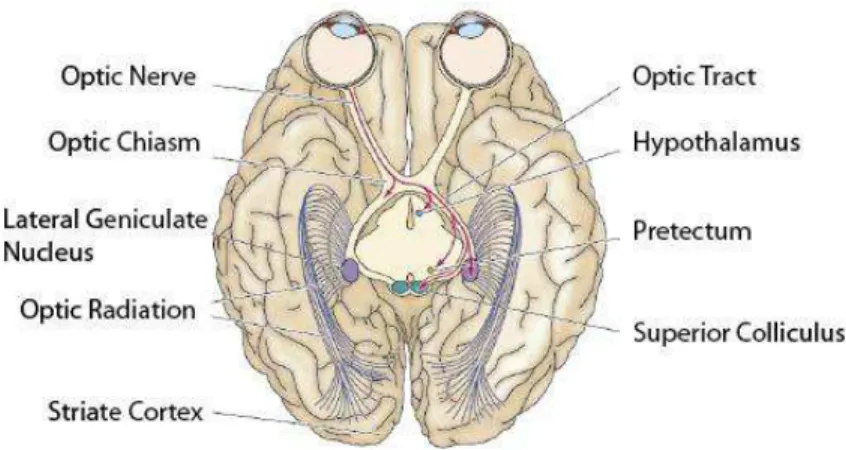
All signal processing starts in the retina, the only peripheral part of the central nervous system and neural portion of the eye. Here, an orderly neural network formed by different kinds of cells (i.e. photoreceptors, bipolar cells, ganglion cells, horizontal cells and amacrine cells) converts the electrical signals generated by photoreceptors into action potentials that will be conducted through ganglion cells axons to the brain (Purves, 2004). The intraretinal circuitry is, by itself, already a highly efficient processing center, sending to the brain encoded information about color, contrast and light changes among many other features. After the signal has left the retina, it travels to the optic chiasm by the ganglion cells axons forming the optic nerve; there, a part of these axons (about 60% in cats and primates) cross the chiasm to the contralateral side of the brain and the remaining part continues ipsilaterally.

Figure 1. Basic connectivity of the visual system from retina to primary visual cortex. [Modified from (Purves, 2004)]

(12)

1. Introduction

10 the dorsal lateral geniculate nucleus (LGN) of the thalamus, which executes relay functions between the optic tract and the primary visual cortex (Figure 1).

Neurons in primary visual cortex (striate cortex or V1) form a well-organized network and are activated according to basic features of simple stimuli (i.e. moving bars with a certain orientation and direction of motion. For details see Section 1.1). These architectural and functional characteristics led researchers to propose that V1 participates in what is considered as low level processing which includes border detection or contour grouping. However whether V1 contributes in more complex visual processing is still an open debate.

The brain’s ability to perceptually separate an object from its background, for example, is a manifold studied mechanism (figure-ground segmentation) where the role of V1 is still not clear. Some features of the connectivity, like the intrinsic long-range horizontal connections, or feedback connections from higher visual areas point out that indeed V1 could play an important role on figure-ground segmentation (see Section 1.2).

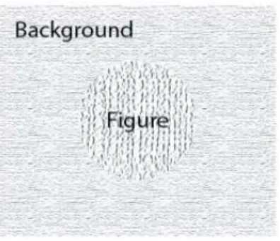
In order to experimentally address the figure-ground segmentation paradigm, researchers train animals (mainly cats and monkeys) to direct the gaze to a specific area on the monitor. The visual stimulus on this area is intentionally designed to perceptually pop out, configuring what is called figure. The remaining area of the monitor is considered as

background (Figure 2). During this task, electrophysiological signals (from single cells activity to population activity) are collected with the intent of better-understand the neuronal correlates of this type of visual processing.

Figure 2. Example of a figure-ground stimulus. The texture of the central circle (figure) was modified to stand out from the background.

(13)

1. Introduction

11 Figure 3. Lateralization of visual pathways. The visual field is divided in two hemifields. The lateral geniculate nucleus (LGN) receives visual input from the contralateral hemifield and transmit it to the primary visual cortex in the ipsilateral brain hemisphere. The interhemispheric connections (IHCs) integrate the information in both hemispheres.

A special kind of connections: the interhemispheric connections, process the visual stimulus located near the vertical meridian (Figure 3) and allows the integration of the hemifields, synchronize the hemispheres, between other important functions. These connections link mainly areas at V1 level, and have a strong functional and anatomical similarity with horizontal intrinsic network. (For details see Sections 1.1.1 and for review Schmidt, 2013).

(14)

1. Introduction

12 In this work we delineate a description of anatomical and functional features of primary visual cortex and its connectivity architecture. We focus on interhemispheric connections and discuss their contribution in visual processing on a figure-ground segmentation paradigm based on spiking and local field potential activity collected from primary visual cortex of anesthetized cats. We frame the discussion in a parallel between long-range horizontal and interhemispheric connections showing that our results are in concordance with the role of horizontal connectivity suggested in the literature, thus strengthening the similarity between the two kinds of connections.

1.1.The Primary Visual Cortex

The primary visual cortex corresponds to Brodman’s area 1 and 1 in the cat . It is

located in the posterior pole of the occipital cortex and constitutes the first cortical stage in visual processing.

The activation of a V1 neuron by direct stimulation is the result of stimulating a spatially restricted area of the visual field. Light changes in different such areas activate different neurons across V1. This portion of the visual field is defined as a classical receptive field of a neuron (CRF) and its main features were well-described by an extensive work of Hubel and Wiesel in the middle of the last century (see Hubel and Wiesel (1959; 1960; 1962; 1963; 1965; 1968).

One of the main functional features of V1 neurons, described by the same authors, is their preference for distinct stimulus moieties. For example, in an experiment stimulating a CRF of a given neuron using moving contrast borders, i.e. bars, there is a specific bar orientation, size and/or movement direction (preferred parameters) that produces the optimal response from that neuron.

Topographically, V1 neurons are arranged in a columnar manner where neurons of the same column share the same properties. Different columns can be defined regarding different response preferences, i.e. neurons in ocular dominance columns receive

(15)

Introduction 1.1 The Primary Visual Cortex

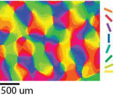
13 Figure 4. Orientation column map resulting from intrinsic signal optical imaging in cat’s V1. Preferred orientation is color-coded according to the scheme on the right. [Courtesy of Dr. Kerstin Schmidt]

As a part of the neocortex, the primary visual cortex is divided in six layers defined by different cell morphology and connectivity. It exhibits three major pathways: The feed-forward connections proceeding from lateral geniculate nucleus to the layer IV, the feedback connections coming from higher visual areas and the intrinsic circuitry, which includes vertical connections from layer IV to II-III and from there to layer V; and also lateral (horizontal) connections within layers, mainly in layers II/III and V (See Section 1.1.1 and Figure 5).

(16)

14 (2000)]. (B) Simplified primary visual cortex connectivity scheme. Layers III and V have a higher concentration of lateral connections (black curved arrows). Extrastriate input (green arrows) arriving from LGN and higher visual areas of the cortex. Extrastriate outputs (red arrows) connecting back to the LGN and to higher visual areas. Vertical circuits (orange arrows) making interlayer connections.

According to Gilbert and Wiesel (1985) the feed-forward connection is responsible for only about 5% of the excitatory input of V1, leaving the most of excitation to feedback and intrinsic connections. Pyramidal projection cells lead the striate output to extrastriate visual areas and basal structures through glutamatergic connections. Neurons from layer VI project back to LGN. Also, layers III and IV project to higher visual areas such as MT, V2 and V5, and layer V projects to the superior colliculus.

Intrinsically, the primary visual cortex makes excitatory connections between (vertical connections) and within layers (horizontal connections) through pyramidal and spiny stellates cells. There is also an intrinsic inhibition network formed mainly by GABAergic basket cells, however, their connection extent is reduced when compared with excitatory connections (Gilbert, 1992).

As a particular group of intrinsic connections in V1 there exist also interhemispheric connections (IHCs), which link topographically corresponding parts of early visual areas on a similar hierarchical level (V1-V1, V2-V2, and V2-V1) in the two brain hemispheres (Schmidt and Lowel, 2002). Based on its anatomical and functional properties, several authors proposed that these connections can be viewed as a continuation of the horizontal intrinsic network (Rochefort et al., 2009; Schmidt, 2013; Schmidt et al., 1997).

Due to the connectivity and response properties of V1 neurons, the functional role, which was initially attributed to this area, was limited to the extraction of basic stimulus features for higher visual areas in which perceptual processing would take place. Currently, this strictly hierarchical conception of visual processing is considered inaccurate since there is evidence that responses of V1 neurons can be modulated by paradigms involving perceptual grouping of segments (Kapadia et al., 1995) and figure-ground segmentation (Biederlack et al., 2006; Ichida et al., 2007; Kastner et al., 1997; Knierim and van Essen, 1992; Lamme, 1995; Levitt and Lund, 1997; Shushruth et al., 2012; Zipser et al., 1996) or brightness perception (Biederlack et al., 2006; Rossi et al., 1996).

(17)

15 contextual modulation (particularly in figure-ground segmentation) and their functional and anatomical similarities with IHCs.

1.1.1. Lateral Intrinsic Connections

Historically, the vertical connections have kept a substantial part of the attention of researchers studying intra-area neural processing. However, many studies indicated the involvement of lateral intracortical connectivity in these processes. A recent study revealed that around 80% of the synapses in a 800μm diameter column stem from long-range axons of neurons located outside that column (Stepanyants et al., 2009) assigning more emphasis to lateral (and feedback) input from outside the classical receptive field. Excitatory long-range intrinsic connections are formed by myelinated collaterals that leave the vertically descending axon trunk before it enters the white matter and can reach up to 8 mm (long-range horizontal connections) (Schmidt and Löwel, 2002). They terminate in a patchy manner, forming clusters of boutons. These terminations cover areas of about 300μm to 600μm in diameter - depending on the labeling technique - and preferentially link columns of similar orientation preference (+/-0 to 30 deg), although columns with oblique (+/-30 to 60 deg) or even orthogonal (+/- 60 to 90deg) preferences can also be connected with decreasing probability (Buzás et al., 1998; Kisvárday et al., 1997; Schmidt et al., 1997). This functional selectivity gives continuity to the network which is likely to contribute to the emergent functional architecture. The modular horizontal network is more prominent in layers II-III and V. Layer IV has shorter and less selective lateral connections, supporting the notion of a different type of processing for that layer (Karube and Kisvárday, 2011; Yousef et al., 1999).

The inhibitory lateral network is about one third to one half of the excitatory network in extent and most of it does not extend farther than 1mm (Schmidt and Löwel, 2002). Its main substrate in the cat’s visual cortex is the large basket cells. Only about 5% of the intrinsic connections are inhibitory, yet their influence cannot be measured by this quantitative view since the GABA dynamics are faster than glutamate, leading to higher inhibition than expected from the number of synapses (Gilbert, 1992). Inhibitory connections are less functionally selective than excitatory ones, i.e. they are more equally distributed between iso-oriented, oblique and orthogonal columns (Buzás et al., 2001) Several functions have been attributed to long-range intrinsic connections like e.g. their contribution to i) adaptive long-term changes in cortical topography after peripheral and central lesions, to ii) dynamical receptive field properties and to iii) contextual influences on classical neuronal responses in V1 (Gilbert and Wiesel, 1992).

Gilbert and colleagues (Das and Gilbert, 1995; Gilbert and Wiesel, 1992) investigated adaptive cortical changes after retinal lesions. The visual cortex contains an orderly

(18)

Introduction 1.1.1 Lateral Intrinsic Connections

16 corresponding cortical area remained initially silenced but its function was altered over time, and was recruited to process a different part of the retina. This process implies not only a topographical reorganization but also changes in the receptive field size as well as its preferences. Therefore, this kind of reorganization was ascribed to the horizontal intrinsic network. Indeed, recently, axonal sprouting of long-range axons has been observed by using 2-photon microscopy in the lesion projection zone (Yamahachi et al., 2009).

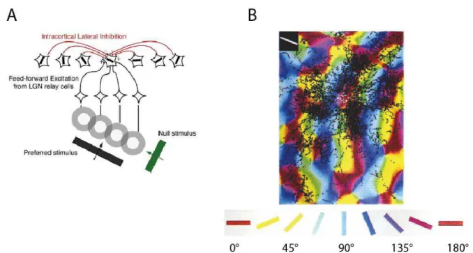
Further, despite some controversy, inhibitory lateral connections have been identified as an important part of the orientation tuning mechanism (Crook et al., 1998; Eysel et al., 1990; Sompolinsky and Shapley, 1997; Wörgötter and Holt, 1991). According to this idea, connections from neurons of nearby columns with other orientation preferences inhibit the response of a given cell to a stimulus with an orientation different from its preferred (see Figure 6). On the other hand, long-range excitatory connections were interpreted to create large composite receptive fields by connecting neurons with similar orientation preferences and synchronizing their responses (Gray et al., 1989; König et al., 1993).

(19)

Introduction 1.1.1 Lateral Intrinsic Connections

17 Considering the above mentioned features (e.g. creating large composite receptive fields, giving continuity to the network, orientation selectivity, part of the tuning mechanism) one would expect that the activity of a given cell is not only determined by stimulation of its CRF (feed forward input) but also by influences from other cells processing different areas of the visual field through the lateral connections. The existence of these influences can be concluded from numerous psychophysical experiments demonstrating that some stimulus’ features presented in the receptive field depend on the context. Figure 7 depicts, how context can alter the perception of the orientation of lines by the presence of nearby lines with different orientation, or also create illusory contours. It was hypothesized that the physiological basis of these phenomena is the input delivered by orientation-selective lateral connections from beyond the CRF (Gilbert, 1992)

Figure 7. Perceptual changes. (A) Apparent orientation changes. [Modified from (Gilbert, 1992)] (B) Illusory contours.

1.1.2. Visual Callosal Connections

Almost all cortical areas of each brain hemisphere are interconnected through the corpus callosum. The excitatory or inhibitory nature of these connections is still on debate, but their exact functional role as well as some of their anatomical features seems to depend on the area they link. Many authors defend that these connections are mainly excitatory (Galaburda, 1984; Geschwind and Galaburda, 1985; Lassonde, 1986; Watson et al., 1984; Yazgan et al., 1995), supporting the idea of integration of cerebral processing between hemispheres (Bloom and Hynd, 2005). Other researchers postulate that callosal connections inhibit the activity between hemispheres (Cook, 1984; Denenberg et al., 1986; Dennis, 1976; Hubel and Wiesel, 1967) contributing to the functional asymmetry (i.e. one hemisphere dominates a given function) present in processes as language and hand dominance.

(20)

Introduction 1.1.2 Interhemispheric Connections (IHCs)

18 meridian (VM) of the visual field is represented (Berlucchi and Rizzolatti, 1968; Lepore and Guillemot, 1982; Ptito et al., 2003). In cats, callosal neurons are mainly pyramidal cells and connect similar classes of cells in supragranular layers (mainly layer III) (Innocenti et al., 1986), however, there is also a limited number of GABAergic projection neurons (Buhl and Singer, 1989; Elberger, 1989).

It is still an open question whether callosal connections are a special kind of long-range horizontal connection or whether they have specific properties related to their positioning within the binocular central visual field, or both. In the primary visual cortex, they were proposed to integrate the cortical representation of the two visual hemifields (Choudhury et al., 1965; HUBEL and WIESEL, 1962) and to synchronize the responses to a visual stimulus across (Engel et al., 1991) and also within the two hemispheres (Carmeli et al., 2007).

Callosal connections share important structural features with intracortical horizontal connections like patchy terminal arbors (Houzel et al., 1994) and linking clusters of neurons sharing similar orientation preferences (Rochefort et al., 2009; Schmidt et al., 1997). The split-chiasm preparation confirmed that indirect input from the callosum matches the direct, ipsilateral responses in orientation and CRF position (Berlucchi and Rizzolatti, 1968; Lepore and Guillemot, 1982; Rochefort et al., 2007).

(21)

Introduction 1.1.2 Interhemispheric Connections (IHCs)

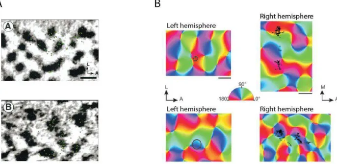
19 was performed in the left hemisphere (black circle) and the corresponding marked synaptic boutons in the right hemisphere (black dots). [Modified from (Rochefort et al., 2009)]

Recent evidence from studies using reversible deactivation of the contralateral hemisphere and thus leaving the visual system intact – in contrast to earlier split chiasm approaches – indicates that the callosal conncetions indeed have a predominantly excitatory integrating function (Makarov et al., 2008; Peiker et al., 2013; Schmidt et al., 1997; Wunderle et al., 2013). Callosal input amplifies responses to ipsilateral CRF stimulation in a multiplicative and stimulus-dependent manner. Inhibitory drives occur highly stimulus-dependent and much less frequent (Wunderle et al., 2013) and the overall balance between inhibitory and excitatory drives matches largely the anatomical numbers given by the intracortical ratio of short and long-range inhibitory/excitatory connections in the primary visual cortex (Kisvárday and Eysel, 1993; Schmidt et al., 2010).

Other functions of visual callosal connections like binocular fusion might arise from their specific localization at the vertical midline of the central visual field but newer studies (Peiker et al., 2011 SFN abstract) confirm that in front-eyed mammals with a large binocular visual field they do not contribute significantly to the ocularity of the interconnected neurons (Minciacchi and Antonini, 1984). Rather, binocular neurons – in contrast to small rodents (Cerri et al., 2010)– seem to be established by the thalamocortical input like anywhere else in the visual field.

A comparison between visual callosal connections and the lateral intrinsic connections (Section 1.1.1) reveals an evident topographical similarity, supporting a strong functional similarity. As opposed to the lateral intrinsic connections the projection through the corpus callosum exhibits the large advantage that its manipulation does not affect directly the recorded neurons (Crook et al., 1998; Girardin and Martin, 2009).

1.2.Contextual Stimulation

(22)

Introduction 1.2 Contextual Stimulation

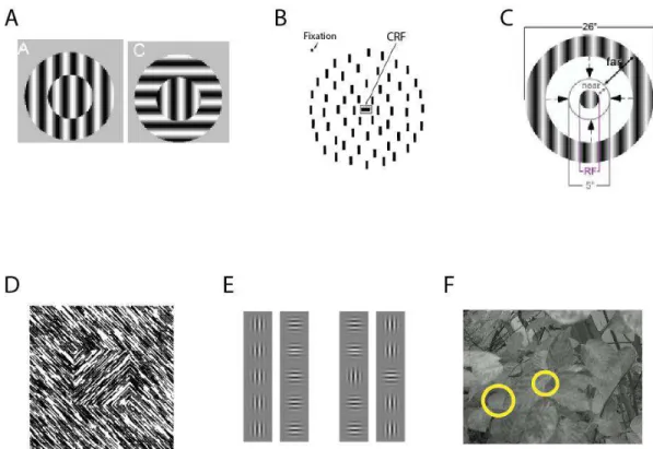
20 square patch embedded by a surround. The patch was made to perceptually pop out as a circumscribed figure by setting differences in the lines' orientation or their direction of motion between figure and surrounding background (Figure 9).

Figure 9. Contextual stimulus. [Modified from Lamme (1995)]. (A) Texture stimulus. A square area was defined to perceptually pop out inside the rectangle’s right half. This is achieved by differences in the line orientations or direction of motion. (B) The small solid square represents the CRF position of a given cell. Upper figure: The CRF is inside the pop-out figure. In this case response facilitation occurred in comparison to the bottom configuration where the CRF was outside de figure.

In the study of Lamme, the facilitation of firing rate occurred only when the CRF was inside the patch and regardless of the orientation preference of the neuron. This finding raised the idea of a perception related processing mechanism (figure-ground segmentation) already at the level of V1 evidenced as response facilitation. Early on, an iso-oriented inhibitory surround was described when stimulating center and surround with iso-oriented stimuli (Allman et al., 1985; Blakemore et al., 1972; Cavanaugh et al., 2002a; DeAngelis et al., 1994; Knierim and van Essen, 1992; Levitt and Lund, 1997; Sengpiel et al., 1997; Toth et al., 1996). However, under different conditions, a facilitation of the center response by iso-oriented surround stimulation had also been observed (Nelson and Frost, 1985; Sillito et al., 1995), although much less frequently.

(23)

21 Whereas the earlier studies were compatible with the view that the bias for iso- versus cross-oriented suppression or facilitation is not fixed but depends on the stimulus orientation presented to the center, newer studies came to a different conclusion. A maximal suppression is gained when the receptive field and surround are stimulated with the same orientation, and less suppression or facilitation by the orthogonal orientation, independent of whether the center is optimally or non-optimally stimulated (Cavanaugh et al., 2002b; Shushruth et al., 2012; Sillito et al., 1995). As this result cannot be explained by fixed orientation-specific excitatory long-range horizontal or feedback connections, a newer theoretical framework proposed a combination of tuned lateral inhibition and weakly tuned local recurrent excitation (Shushruth et al., 2012). Long-range lateral and feedback circuits would have a context dependent and modulating role on this local recurrent circuit which enables the neurons in the center/foreground of the stimulus to flexibly adapt to the changing feed-forward input.

(24)

22

The debate of whether contextual modulation depends or not on a neuron’s preferences is

based on the activity of single cells. However, since the cortex is a complex network of interconnected neurons, there is growing evidence of stimulus processing at the population level. It was postulated for example that neurons in V1 representing the same object fire in synchrony (Singer, 1993). This proposal is based on the idea of neuronal assemblies introduced by Donald Hebb in 1949 and considers groups of neurons firing together as the elementary unit of information processing, in contrast to the idea of having a single cell to represent each object (Barlow, 1972). In this case, the neuronal representation of a given object is a group of cells firing synchronously, with each cell having the possibility of representing a different basic object feature. This is the base of the binding-by-synchrony theory which considers ensemble synchronization as an effective way of cortical information (Von der Malsburg and Shneider, 1986; Singer, 1994; Hopfield, 1995; Vaadia et al., 1995). Nevertheless, the network mechanism to synchronize the responses of different neurons is still not clear. One hypothesis is that the key of this synchrony could be at the local field potential level, since this signal is the result of the summation of the activity of a neuronal population. More specifically, a group of neurons fire together if they share preferences to discharge, for example, at a particular phase of a local field potential (LFP) wave (Siapas et al., 2005).

However, there is also evidence against this binding-by-synchrony theory showing that simultaneously recorded neurons, with receptive fields stimulated by the same object, fail to synchronize their responses (Lamme and Spekreijse, 1998; Roelfsema et al., 2004). Instead, Roelfsema and colleges gave experimental support to a binding-by-rate enhancement hypothesis where the neurons encoding features of the same object jointly enhance their responses.

There is also evidence that different coding strategies might exist in parallel. Biederlack and colleagues (2006) used sinusoidal gratings stimulation on anesthetized cats. Whereas orientation contrast led to an increment of firing rate, phase contrast produced an increase in synchrony, suggesting that, depending on certain stimulus features, the figure-ground segmentation could have different electrophysiological correlates.

Taken together, these studies agree with the notion that figure-ground segmentation takes place already at early visual areas, yet the electrophysiological correlates and relations between those and specific stimulus features remain controversial.

In the current thesis, we explore changes in neuronal responses (i.e. spiking activity and

(25)

23 principle deactivates all connections between the two visual cortices, not only the callosal ones though the callosal projection is likely to be the dominant interhemispheric link for the visual system.

(26)

2. Working Hypothesis

24

2. Working Hypothesis

I. Since there is evidence of figure-ground segmentation in population activity, we thus also expect evidence of that process in LFPs and assembly activity.

(27)

3. Objectives

25

3. Objectives

- Evaluate LFPs evoked by uniform whole-field stimulus in comparison with a stimulus which creates a perceptual pop-out by means of an orientation contrast (gratings) or a motion contrast (natural scene)

- Evaluate coordinated activity of groups of neurons, i.e. assembly activity.

- Evaluate synchronization between LFPs and single unit or assembly activity reflected in phase-locked events.

(28)

4. Materials and Methods 4.2 Recording Area Identification

26

4. Materials and Methods

Nine adult cats (labeled as Ca07, Ca10, C11, C12, C15, C27 and C28, C29 and C31, 4 males and 5 females) were prepared and maintained under anesthesia and artificially ventilated during the experiments. Experiments Ca07-C15 were performed at the Max Planck Institute for Brain Research in Frankfurt, Germany, the remaining four experiments were performed at the Brain Institute of the UFRN in Natal. All procedures were approved by the

local animal right’s authority at the Regierungspräsidium Darmstadt in the state of Hessen,

or by the ethic committee of the Federal University of Rio Grande do Norte in Natal (UFRN). 4.1.Anesthesia and Physiological Monitoring

Initially, all animals were anesthetized by intramuscular injection of 10 mg/kg ketamine hydrochloride and 1 mg/kg xylazine hydrochlodride. Subsequently, they were artificially ventilated with a mixture of 0.6/1.1 % halothane (for recording/surgery respectively) and N2O/O2 (70/30%). After completion of surgical procedures and during the entire

experiment, the animals were maintained paralyzed by continuous intravenous infusion of pancuronium bromide (0.15 mg/kg/h). The physiological stability of the animals during anesthesia was evaluated by continuously monitoring the electrocardiogram and CO2 levels

in the expiration air. During all experiments we aimed to keep the heart rate between 100 bpm and 170 bpm and the CO2 output between 2.5 and 3.7 %mmHg.

4.2.Recording Area Identification

(29)

4. Materials and Methods 4.2 Recording Area Identification

27 Figure 11. Intrinsic signal map. Left: Map obtained from vertical gratings stimulation. Center: Map obtained from horizontal grating stimulation. Right: Photo of the cortex area exposed. The markers indicate a possible location for electrodes implantation. These points were selected for displaying a clear response to the stimulation (orientation columns). White and black markers are used just for contrast matters with no color-coding involved.

4.3.Electrode Implantation

(30)

4. Materials and Methods 4.5 Cooling Procedure

28

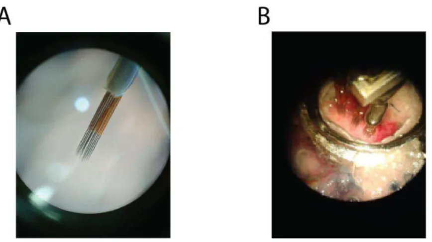
Figure 12. (A) Electrode matrix (4x4, 250µm between electrodes) (B) Recording chamber and three implanted matrixes. Both photos were taken through the microscope lens.

4.4.Stimuli

Two stimuli categories were presented during the experiments (square gratings and natural scenes) in two different configurations (whole-field -WF- and Patch). The Patch configuration was defined by selecting an area (which defines the figure) to perceptually pop-out by setting an orientation or direction of motion contrast between the figure and the surrounding area (ground).

In the case of grating stimulation (all experiments), the WF configuration consisted of two sets of 4 full-field gratings oriented clockwise in steps of 45 degrees moving in one of the two directions perpendicular to the bars orientation. The Patch configuration consisted of the same eight full-field gratings containing a squared grating patch (12deg x 12deg of visual field angle) with an orthogonal surround also moving in one of the two directions perpendicular to their own orientation (see Figure 13A). All gratings had the same spatial and temporal frequency with parameters adapted to the response properties of the majority of the recorded neurons in the respective sample (area 18: 0.15 cyc/deg and 16 deg/sec).

(31)

4. Materials and Methods 4.5 Cooling Procedure

29 Figure 13. Examples of the two stimulus categories. (A) Square gratings in two different configurations: WF (upper sketch) and Patch (lower sketch). (B) Natural scene. Same conventions as in (A). Red arrows indicate the direction of motion. The complete set of conditions for each stimulus category is depicted in Supplementary Figure 1.

4.5.Cooling Procedure

(32)

4. Materials and Methods 4.6 Data Recording

30 Figure 14. Cooling setup. [Taken from (Wunderle, 2012)] (A) Cooling probe with a thermocouple attached. (B) Cooling system. Chilled methanol is pumped through the system while the probe temperature is monitored.

4.6.Data Recording

Both recording and stimulus presentation were accomplished using custom software in LabView (MEC and SPASS by S. Neuenschwander). In a first step, a CRF mapping was performed by stimulating with a single bar oriented in 22.5° steps moving in the perpendicular direction (16 conditions). For each condition a peri-stimulus time histogram (PSTH) was computed in order to identify the variation of spiking activity over time. After considering all conditions and knowing the position of the bar at the PSTH's peak time, we could infer the area of the visual field that, when stimulated, produced the response of the measured channel (Fiorani et al., 2014).

(33)

4. Materials and Methods 4.7.1 Orientation Tuning of Multiunit Activity

31 Figure 15. Stimulation scheme of a single recording. After the data acquisition starts there is a 250ms blank interval followed by 250ms of static and 1500ms of moving stimulus.

Subsequently, the right hemisphere was cooled and after temperature stabilization a new recording session was executed (cooling, see Section 4.5). The cooling session was followed by a resting period of 40min to recover normal cortical temperature and stabilize responses until a third and final recording period was performed (recovery).

4.7.Data Analysis

All data analysis was performed using the Matlab signal processing toolbox and customized codes to read from LabView, organize, select and analyze the recorded data. As pre-processing procedure all recordings were visually inspected in order to identify and discard possible damaged recording sites or artifacts.

4.7.1. Orientation and Direction Tuning of Multiunit Activity

In order to define selection criteria we characterized the multiunit activity from each recording site according to three main parameters: Receptive field position (see Section 4.6), orientation preference, and direction of motion preference; the last two defined by an angle and a tuning index. The tuning index was calculated by equation 1, i.e. by vectorial addition of spike counts across all trials,

√ ∑ _∑ ∑ | | (1)

where Tuning Index can be an orientation index (OI) or a direction index (DI), R(θi) is a vector with magnitude equal to the accumulated spike count as response to condition i

(34)

4. Materials and Methods 4.7.3 Assembly Detection

32 response (if any) to all conditions, and the second the ideal case where the unit responds only to a single condition.

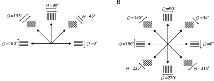
Figure 16. Correspondence between stimulus conditions and angles. (A) Angles for OI computation. Note that stimulus conditions with the same orientation contribute to the same vector regardless of the direction of motion. (B) Angles for DI computation. Note that stimulus conditions with contrary direction of motion contribute to opposite vectors. In both cases, the resultant is the vectorial sum across all trials normalized by the sum of all responses.

4.7.2. Firing Rates and Power Spectral Density

First, for each stimulus condition, the mean firing rate (FR), defined by equation 2 was computed for each recording site as a response to each stimulus condition.

∑ |

(2)

where denotes the mean firing rate during the presentation of stimulus condition , computed by adding the spike counts obtained in each trial of in the moving period of the stimulation (see Figure 15) between t0=500ms and t1=2000ms. This value

was normalized by the length of the moving period T=1500ms.

(35)

33

(3)

∫

(4)

Where denotes the Fourier transform of time series defined in equation 4 (in this case the LFP signal), denotes frequency and is the conjugate. There are several methods to compute the PSD. Here the Welch’s method was used which calculates an average of periodograms obtained from several overlapping time windows across the signal, reduces the noise and provides a good PSD estimate. For these calculations a Hamming window of 250ms with 50% overlapping and a frequency resolution of 0.5Hz were defined.

In a study of awake cats, visually stimulated with sine gratings, Kayser and colleagues (2004) suggested that temporal and structural stimulus features could be locked to the power of different frequency bands (23Hz to 36Hz and above 109Hz for temporal features and 8Hz to 23Hz and between 36Hz and 109Hz for structural features). Based on this finding, in addition to qualitative inspection of PSD from our data (see Figure 17), we computed the power (defined as the area under the curve) of three different frequency bands: 10-20 Hz (Alpha), 20 – 50 Hz (Low Gamma) and 50 – 90 Hz (High Gamma) (Niessing et al., 2005). From now on, we’ll use the abbreviations LG and HG to denote low gamma and high gamma rhythms respectively.

Figure 17. Representative examples of four PSD. Obtained from different cats at recording site

(36)

34 In order to quantify the figure-ground segmentation an index was defined as follows:

(5)

where is the segmentation index, denotes the magnitude of the neuronal response

FR or LFP band’s power to a given Patch condition, and denotes the magnitude of the same response to the WF condition. Since we aim to quantify the effect of surround, the SI

was computed just for WF-Patch responses pairs that maintained the same stimulation of the CRF (feedforward input) between the two conditions. The SI ranges from -1 to 1 with more positive values indicating higher responses to Patch stimulation.

To quantify the IHCs deactivation effect on neuronal responses FR or LFP band’s power , a cooling index was defined as:

(6)

where is the cooling index, denotes the response magnitude to a given condition (WF or Patch) during Baseline recording and denotes the same response during cooling recording. This index also ranges from -1 to 1 with positive values indicating a response increase in the absence of interhemispheric input and negative values indicating a response decrease during the same recording. Note that response increases during cooling indicate the release of inhibitory influences in the intact system and decreases indicate the release from excitatory influences.

4.7.3. Assembly Detection

According to the Hebbian theory any two cells that are repeatedly active at the same time

will tend to become associated, so that activity in one facilitates in the other (Hebb, 1949);

this process results in groups of neurons with the tendency to fire together known as neuronal assemblies. In order to identify such a tendency it is necessary to isolate the activity of single neurons. As our spiking data from each recording site could originate from more than one neuron, a spike sorting method was necessary, however, in order to track the activity of single units along the entire experiment, we first concatenated the spiking data from baseline, cooling and recovery recording periods before sorting. We used

(37)

35 Figure 18. General overview of the construction of the normalized rastergram Z and autocorrelation matrix computation. [Modified from (Lopes-dos-Santos et al., 2011)] (A) Rastergram. Each line represents a neuron and each mark denotes an action potential (spike) (B) Five milliseconds bins were defined and the spikes inside each bin were counted resulting in the binned spike activity. (C) Spiking activity normalized by z-score. (D) Autocorrelation matrix. Each element is computed by linear correlation of a pair of neuronal activity (lines)

The spiking times of single units were organized into a rastergram (Figure 18A) where each line corresponds to a single cell’s activity. Then, the rastergram was binned using 5ms non-overlapping time windows counting the number of spikes in each bin (Figure 18B). The binned rastergram was z-scored in order to normalize each neuron’s activity obtaining zero mean and unit variance for each row (Figure 18C).

(38)

36 the number of assemblies based on the eigenvalues of the autocorrelation matrix of Z. If Z is a random matrix (i.e. without ensemble activity) these eigenvalues follow the Marcenco-Pastur distribution defined in equation 7.

√ (7)

where ⁄ , is the standard deviation of the elements of Z (since Z is the result of z-score normalization, in this case ; and are defined by:

_√_⁄ (8)

If Z is not random (i.e. contains ensemble activity), some eigenvalues of its autocorrelation matrix lie outside the theoretical boundaries determined by equation 8 (see also Figure 19), with the number of eigenvalues above the upper boundary (Nas) indicating the number of assemblies in Z.

(39)

37 Figure 19. Examples of Marcenko-Pastur distributions [Modified from (Lopes-dos-Santos V et al. 2011)]. (A) Left: Binned spiking activity of 20 simulated independent neurons. Right: Theoretical Marcenko-Pastur distribution (up) and eigenvalues distribution (down). Note that the eigenvalues follow the Marcenko-Pastur distribution. (B) Left: Binned spiking activity of 32 simulated neurons. Three assemblies were artificially defined (assembly 1: neurons 4 to 7, assembly 2: neurons 10 to 13 and assembly 3: neurons 26 to 29). Right: same as (A). Note that in this case there are three eigenvalues above the upper boundary of the Marcenko-Pastur distribution matching the number of assemblies simulated.

(40)

38 Figure 20. Assembly pattern and assembly activation along time. The figure shows a 1500ms length rastergram representing the spiking activity of 44 neurons during one trial. Right: Assembly pattern. Each neuron (lines in the rastergram) is associated with a weight value. Neurons with high weight are more likely to participate in the assembly activity. Lower trace: Projection of the assembly pattern on the spiking activity in each time bin. The assembly is considered active when its projection exceeds a threshold (dashed black line). Note that the firing rate of neurons with high weight (within the dashed white squares) simultaneously increases at the time bin the assembly activity reaches threshold (orange dots).

As a last step, each pattern was projected along the rastergram in order to quantify the

assembly’s activation on each time bin. At a given time bin, the more similar the bin and assembly patterns are, the higher the values of the projection will be, thus indicating stronger assembly activation. In order to define specific times of activation it was defined that the assembly is active in time bins with projection values above the percentile 99.

4.7.4. Phase Locking

(41)

5. Results 5.1 Recording Sites Characterization

39 Figure 21. General overview of phase locking analysis. (A) Filtered LFP in three different frequency bands (Alpha, LG and HG). Short black lines at the bottom indicate the occurrence of a spike event in time (i.e. a spike from a single cell or assembly activation). For each time point, a phase of each rhythm is extracted (black dots) (B) Detail from grey square in (A). (C) Illustrative examples of two phase distributions. Upper histogram: uniform distribution indicating no phase preferences. Lower histogram: Non-uniform distribution showing preference for an occurrence of a

spike event in moments when the LFP’s phase is around π radians.

(42)

40 Figure 22. Von Mises distribution for different K values. Note that the higher the K the narrower the distribution. The x-axis corresponds to radians and y-axis to probability. [Obtained from

http://en.wikipedia.org/wiki/Von_Mises_distribution]

(43)

41

5. Results

5.1. Recording Sites Characterization

We recorded and inspected a total of 544 recording sites from sixteen different datasets (a new dataset was defined by lowering the electrodes at least 150µm into the cortical surface from the previous recording depth; see Table 1) from which a set of 406 sites presented a well-defined receptive field (Figure 23A. Left).

Table 1. Number of datasets and recording site for each cat

Cat Code Number of datasets Number of recording sites

Ca7 1 16

Ca10 2 32

C11 1 32

C12 1 32

C15 2 64

C27 1 32

C28 3 96

C29 3 144

C31 2 96

(44)

42 Figure 23. Recording sites characterization. (A) Left: Example of recording sites with well-defined CRFs, inside the patch area. Right: Tuning polar plot from the same recording site. OI stands for orientation tuning. Note that the multi-unit is highly orientation selective. (B) Example of tuning polar plot, from another recording site, revealing high selectivity to direction of motion. DI, direction selectivity index (C) Example of a poorly selective recording site according to all criteria. In all plots the outer circle is scaled to the maximum number of spikes (upper left).

In case of grating stimulation we selected recording sites which were highly selective to orientation stimulation and whose CRF was inside the patch area (n=205, mean OI: 0.47+/-0.17 SD) aiming to consider the optimal responses from each recording site. Since the

(45)

43 Figure 24. Orientation and direction of motion preferences. Bars represent the number of recording sites during baseline (orange) and cooling (blue). Dashed gray lines correspond to line

x=y (A) Orientation preference. (B) Orientation index. (C) Direction of motion preference. (D) Direction index.

(46)

5. Results 5.2 Raw Responses

44 As expected for the areas we are recording from, our sample was less selective to direction of motion than to orientation. The data distributions in Figure 24C and D suggest a higher influence of interhemispheric connectivity on direction selectivity than on orientation selectivity but changes in direction of motion parameters were also not significant.

These results are in line with previous reports stating that orientation and direction selectivity examined with gratings do not change drastically in the absence of interhemispheric input and that direction selectivity is –if at all- stronger influenced (Schmidt et al., 2010; Wunderle et al., 2013)

5.2.Raw Responses

(47)

45 Figure 25. Representative examples of responses to preferred condition during grating stimulation. (A) Mean power spectrum density (B,C) Mean peri-stimulus time histograms (PSTH). All plots depict responses to Patch (red) and WF (green) stimulation during baseline (orange), cooling (blue) and recovery (grey). (B) Response facilitated by Patch stimulation. (C) Response suppressed by Patch stimulation. Note that the facilitated response was more affected in the absence of interhemispheric input than the suppressed response. Shades represent standard error.

On average, we found that Patch conditions evoked less spikes than WF conditions during baseline (paired T test p<0.05) and cooling (paired T test p<10-3_{) (see Figure 26C). In}

contrast, the power of Alpha and LG bands was lower during WF stimulation in comparison to Patch stimulation (paired T test p<10-3_{, Figure 26D and}_p_{<0.05, Figure 26E respectively)}

during baseline. Noteworthy, only the LG’s power difference between WF and Patch

(48)

46 Figure 26. Grating stimulation. Averanged responses (n=205) to preferred whole-field (WF) and Patch conditions during baseline (orange), cooling (blue) and recovery (gray). (A)Mean firing rates for 205 multi-units. (B) Mean Alpha power. (C)Mean Low Gamma power. (D) Mean High Gamma power. Statistical test: paired T-test (*) significance level p<0.05; (***) significance level p<10-3_.

Note that the relation between WF and Patch response almost reverses in the absence of IHC input for the LG band.

(49)

5. Results 5.3 Segmentation and Cooling Indexes

47 Figure 27. Representative examples of responses to preferred condition during natural scene stimulation. (A) Power spectrum density. Note the rebound of Patch gamma activity in the recovery. (B,C) Mean peri-stimulus time histograms (PSTH). Conventions as in Figure 26. (B) Response facilitated by Patch stimulation. (C) Response suppressed by Patch stimulation. Note that the facilitated response was more affected in the absence of interhemispheric input than the suppressed response. Shades represent standard error.

On average, during baseline (Figure 28) we only observed differences in firing rates for WF and Patch (paired T test p<10-3_{). Here, the power differences observed for LFPs obtained}

with the two different grating stimuli above were not present. Yet, during the deactivation of IHCs, both firing rates as well as Alpha and LG power were lower for Patch conditions (paired T test p<10-3_{) similar to the result obtained with gratings.}

(50)

48 levels but can lead to yet another activation state (Wunderle, Schmidt, personal communication)

Figure 28. Natual scene stimulation. Averaged responses (n=184) to preferred whole-field (WF) and Patch conditions during baseline (orange), Cooling (blue) and Recovery (gray). (A) Firing rates.

B Alpha’s power. C Low Gamma’s power. D High Gamma’s power. Statistical test: paired T-test (***) significance level p<10-3_{. Note that LFP power differences between WF and Patch stimulation}

are not present in the baseline but are disclosed by deactivation of IHCs and are maintained in the recovery period (significant for the LG band)

5.3.Segmentation and Cooling Indices for firing rates and LFPs

(51)

49 the IHCs deactivation effects separately on the two conditions, Patch (cross-oriented) and WF (iso-oriented) (see Equation 5 and 6 in Methods, section 4.7.2).

Figure 29. Segmentation and cooling indices of firing rates. (A) Results from grating stimulation (i) Averaged segmentation index of the same set of recording sites (n=205) during baseline, cooling and recovering. (ii) Segmentation index correlation plots and histograms for the individual recording sites during baseline (orange) and cooling (blue). In the correlation plot, each point represents one recording site. (iii) Cooling index from responses to WF and Patch stimulation of the same set of recording sites. (B) Results from natural scenes stimulation. (i) (ii) and (iii) as in (A). All bars represent the mean +/- standard error of each distribution. Statistical test: paired T-test. (***) significance level p<10-3_{. Rec. Sites stands for recording sites.}

(52)

50 suppression or less excitation for the Patch as opposed to the WF condition in the absence of interhemispheric input. The analysis of CI revealed that, on average, the effect of IHCs deactivation was more accentuated on Patch responses than on WF responses (firing rate mean reduction of 23.7% and 19.02% respectively, Figure 29Aiii, paired T-test, p<10-3_).

This explains the SI variation depicted on Figure 29A and indicates that the decrease of the SI is a result of a higher loss of excitation for the Patch than for the WF condition when removing IHCs.

Despite that on average (negative SI in Figure 29i), the firing rate for iso-oriented surround (i.e. WF) was slightly higher than the firing rate for orthogonal surround (i.e. Patch), the histogram in Figure 29Aii reveals that during baseline the contrary is also frequent, resulting in a nearly symmetric distribution of SI values (orange; 55% of negative SI and 45% of positive SI). The plot in Figure 29Aii also points out that there is tendency of recording sites with negative SI during baseline to be more affected by deactivation of IHCs. Figure 29B demonstrates the SI and CI results from natural scene stimulation. Overall tendencies are similar to grating stimulation (compare Figure 29A). Firing rates are on average higher for WF stimulation, i.e. iso-oriented surround, than for Patch stimulation, i.e. cross-directed surround movement. Deactivation of the contralateral hemispheres enhances that tendency mainly by removing more spikes for stimulation with the Patch than with WF condition (firing rate mean reduction of 34.8% and 33.7% respectively). However, overall, the SI and CI decreases are stronger for that stimulus category than with gratings. This goes along with an earlier observation that responses to stimuli which are less salient than gratings reveal more integration by the lateral networks and thus predominantly decrease their spike rates during deactivation of IHCs (Wunderle et al., 2013).

We next considered the power of Alpha, LG and HG frequency bands. Computation of SI indices for grating stimulation revealed, on average, more power in Alpha and LG bands for Patch as compared to WF conditions, during baseline (positive SI in Figure 30Ai, Bi and Ci). This in contrast to the average negative SI indices observed with firing rates Figure 29) but one should note that average SI indices are rather small in all cases as confirmed by the histograms (Figure 29ii, 28ii, 29ii) of the individual SI indices showing that facilitative and suppressive effects are quite balanced in our sample.

(53)

51 Figure 30. Segmentation and cooling indexes of LFP’s power for grating stimulation. Results in the Alpha (A), LG (B) and HG (C) band from grating stimulation. Conventions as in Figure 29.

(54)

52 Figure 31. Segmentation and cooling indexes of LFP’s power for natural scene stimulation. Conventions as in Figure 29.

Taken together, we observed that in a population of neurons located at the cat’s 1 /1

border responses to a pop-out patch condition tend to be lower than to a uniform

(55)

5. Results 5.4 Assemblies Detection and Characterization

53 Interestingly, we observed that for that stimulus category, the SI had a tendency to fall in function of the frequency increase of the considered response.

Figure 32. Variation of segmentation index in function of the response’s frequency. During the presentation of gratings (A) and natural scenes (B). LG: Low Gamma. HG: High Gamma. Statistical test: T-test (***) significance level p<10-3_.

5.4.Assembly Detection and Characterization

The above results so far are compatible with the interpretation that figure-ground segmentation involves also other mechanisms than a mere generalized increase or

decrease of firing rates or LFP’s power in primary visual cortex. In fact, other studies showed that synchrony processes at single unit or LFP levels (Biederlack et al., 2006; Gail et al., 2000) can also play an important role for figure-ground segmentation. In order to define an approach that examines the population activity of the in parallel recorded neurons focusing on the foreground patch we evaluated the activity of neuronal assemblies. Aiming to characterize these assemblies we followed a similar analysis described for individual recording sites. As a first step, we computed an extended version of the CRF mapping in order to identify that part of the visual field which could strongly influence the activity of each assembly (i.e. the joint receptive field –JRF- formed by the CRFs of the more active –highly weighted- neurons in the assembly).

For each assembly pattern, we constructed N two-dimensional Gaussians (N= number of neurons), centered at the CRF of each neuron, with standard deviation equal to the area of its CRFs and an amplitude equal to the neuron’s weight in the pattern. The JRF is defined as the mean of all Gaussians and is centered at its maximum value (Figure 33). Depending on

(56)

54 Table 2 presents general information about the assemblies detected during grating and natural scene stimulation.

Figure 33. Joint receptive field computation. (A) Upper row: Receptive fields (red rectangles) of three neurons belonging to the assembly pattern at the bottom. Here, for a matter of visualization, we only depicts the CRF for those neurons, however the calculations were performed for all units. (B) Based on the center of the receptive field of a given unit i (xi,yi) and its area Ai, we constructed a two-dimensional Gaussian centered at (xi,yi), with standard deviation Ai and amplitude Wi equal to the neuron’s weight in the assembly. (C) The joint receptive field (JRF) by calculating the mean of the Gaussians obtained in B. Depending on the location of its center (white x), we classify the assembly as figure-driven or ground-driven.

Table 2. _{Assemblies’ characterization.} Stimulus Neurons per

recording site

Neurons per data set [min

max]

Assemblies per data set

Figure-driven assemblies

Ground-driven assemblies

Grating 1.47 [22 60] 9.33 100 60

Natural Scene 1.84 [38 60] 11.1 60 51

Since we identified the activation times (and thus, the number of activations) during the presentation of each condition of gratings stimuli (see Figure 20 in Methods section), we could characterize each assembly in terms of its orientation and direction of motion preferences by the calculation of the direction and orientation indices (Figure 34). Based on these parameters, we considered only figure-driven assemblies with an orientation index higher than 0.2 for all further analysis regarding grating stimulation (n=76).

(57)

55 directions). Instead, we identified the preferred of all the four WF conditions, and selected figure-driven assemblies and their response to that preferred condition.

Assemblies observed with grating stimulation revealed a clear preference for one of the four orientations presented with the stimulus, rather than being distributed across all possible interpolated orientations (Figure 34A). We also noticed a slight bias to the vertical orientation. This was to be expected considering that this bias was already present in the orientation preference distribution of the individual recording sites (see Figure 24). Deactivations of IHCs did not affect significantly the orientation preference of the assemblies; however, it significantly increased their orientation index (paired t-test,

p=0.009, Figure 34B)