•
•
"
..
... #"FUNOAÇÃO ... GETULIO VARGAS
EPGE
Escola de Pós-Graduação em Economia
,
SEl\llNARIOS
DE PESQUISA
ECONÔMICA
" Conditional Labour
Supply, Quantile Functions
in Brazil."
Prof
o
Eduardo Pontual Ribeiro
( Universidade Federal do Rio Grande do Sul)
LOC.-\L
Fundação Getulio Vargas
Praia de Botafogo, 190 - 10° andar - Auditório
D\T\
23/04/98 (5:1 feira)
HOR-\RIO
16:00h
•
•
Conditional Labor Supply Quantile Estimates
InBrazil
t
Eduardo Pontual Ribeiro
Departamento de Economia, Universidade Federal de Roraima and
CPGE, Universidade Federal do Rio Grande do Sul Porto Alegre, RS, 90040, Brazil
e-mail: [email protected]
This version: August, 1996; Revised: February, 1997.
Keywords: Labor Supply; Quantile Regression; Structural Models. JEL Classification: C13; C31; J22.
"--,
I J
,
•
lo
..
..
Abstract
The estimation of labor supply elasticities has been an important issue m the economic
literature. Yet all works have estimated conditional mean labor supply functions only. The objective of this paper is to obtain more information on labor supply, by estimating the
conditional quantile labor supply function. vI/e use a sample of prime age urban males
employees in Brazil. Two stage estimators are used as the net wage and virtual income are
found to be endogenous to the model. Contrary to previous works using conditional mean estimators, it is found that labor supply elasticities vary significantly and asymmetrically
across hours of work. vVhile the income and wage elasticities at the standard work week are
zero, for those working longer hours the elasticities are negative.
Resumo
A estimação de elasticidades de oferta de trabalho tem sido um tópico importante na
lit-eratura econômica. Todavia, todos os trabalhos até hoje têm estimado funções de oferta
de trabalho baseados na média condicional apenas. O objetivo deste artigo é obter maiores
informações a respeito da oferta de trabalho, via a estimação dos quantis condicionais da
oferta de trabalho dos trabalhadores urbanos no Brasil. Estimadores de dois estágios sào empregados devido a evidência que o salário liquido e a renda virtual sào endógenos no
mod-elo. Ao contrário de trabalhos anteriores baseados em estimadores da média condicional.
os resultados indicam que as elasticidades de oferta de trabalho variam significativamente
e que são assimétricas ao longo das horas de trabalho. Enquanto as elasticidades renda e
salário na jornada de trabalho padrão de 40 horas são zero, para aqueles que trabalham
•
1
Introduction
The study of the individual responses in \vork hours to changes in wages and nOIl-labor income occupies a significant portion of the economic literature, with many developments in the estimation methodology, as can be seen in the surveys of Haus-man (1985), Pencavel (1986) and Ki11ingsworth's (1983) monograph. While these developments have contributed to the understanding of the labor supply of economic agents, only conditional mean estimates have been obtained. These conditional mean estimates suffer fram the limitations that are heavily influenced by the high concen-tration of \Vork hours at the standard work week (genera11y at 40 and 44 hours). and do not convey the actual variability of responses in the sample.
The objective of this work is to present a methodology to obtain sim pIe and direct estimates of the complete conditional labor supply function across work hours, us-ing a robust semiparametric estimation method, namely Quantile Regression. This estimator, introduced in Koenker and Bassett (1978), complement conditional mean (Least Squares or Ma.ximum Likelihood) results. praviding a more complete and accurate description of the model. Quantile Regression 'has not received the atten-tion it deserves' (l\Ianski, 1991, p.45), and has been used mainly on wage studies so far (Buchinsky, 1994, 1995, and others), uncovering interesting results of varying responses to the covariates across the distribution of the dependent variable.
The methodology is applied to a sample of prime age urban employees in the private sector in Brazil, using data fram the 1990 PNAD. estimating previously unknown estimates of labor supply elasticities. A one period utility maximization model is used and income taxes are taken into account on the budget constraint. Possible endogeneity of the wage and income variables impose the use of T\','o Stage estimators, where these variables are instrumented. Both Tv"o Stage Least Squares (2SLS) and, introducing in the labor supply literature, Two Stage Regression Quan-tiles (2SRQ) are used.
The paper is organized as fo11ows: the description of the labor supply model and the empirical specification fo11ows this introduction. The estimators, in particular quantile regression, are presented in the third section, with the data set used de-scribed in the section afterwards. The fifth section presents the results and the last section concludes.
2
Labor suppIy specification and empirical modeI
•
"
ED are exemptions and deductions. Individual behavior is assumed consistent with the utility maximization axioms and the utility function U(m, L - h) is taken to be strictly quasi concave.
U nder a progressive income taxo as is the case in Brazil. the ta..'<: rate t increases \vith taxable income across the j = 1, ... , m brackets. The effective marginal wage rate is given by the net wage rate Wj = w(l - t)). The marginal wage decreases as hours increase so that the budget constraint is piecewise linear. In addition. the (extended) intercept of each segment, that is, the income at zero hours of \\'ork has to be adjusted. This extended intercept is denoted virtual income (vy) o and is such that it corrects the non-Iabor income for the taxation of part of income at lower rates (Killingsworth, 1983). The now linearized budget constraint can be written as
wh+vy = m. Note that the budget set is still convex, guaranteeing unique solutions for the maximization of quasi-concave utility functions.
It is assumed that the preferences can be represented by a Stone-Geary util-ity function (Rosen, 1978, Killingsworth, 1983), aIs o denoted Linear Expenditure System (LES)l The problem faced by each individual is to maximize
U(m, L - h) = (1 - ah)ln(m - c)
+
ahln(L - h), (1)over h, m ~ 0, constrained by wh
+
vy = m. The relative preference for non-work hours. 1>
ah>
0, and m>
c ~ O, the minimum leveI of goods consumption are parameters of the utility function.The labor supply function obtained from the maximization problem is
(2)
The main advantage of this parametric form is that it allows a nonlinear response to wages, and does not constrain the sign of the wage effect. Backward bending labor supply curves depend on the leveI of c and vy, for given wage and income parameters. Further. it can be understood as simple 'rule of thumb o behavior: individuaIs choose hours so to obtain a certain earnings, as a weighted average of non-wage income and the value of leisure endowment (Lw). This is easily seen by rewriting the labor supply function as wh = (1 - ah)Lw - ah(vy - c).
In the empirical specification, assume that the minimum subsistence levei of income Ci of each individual i=l, ... ,n is a function of demographic characteristics
(Zi): Ci = c
+
K,Zi. This form of heterogeneity is justified in that not all individuaIsnecessarily have an identical minimum subsistence leveI. For example. it is clear that the consumption leveIs change across age groups and that the presence of children in the household would increase the minimum income requirements. Second. assume
•
•
that the number of hours available for work across individuaIs can be approximated by Li = L
+
uLi, where L is a common measure of hours across the population and ULi is an íid(O,O"d random variable, uncorrelated with the independent variablesw, vy and Z. Finally, allowing for possible heterogeneity of wage and income effects. the estimating equation may be written as
. 1 , VYi Zi,
hi = CXo -r CXl - -r CX2-
+
CX3- -r E,:Wi Wi Wi (3)
where Ei is a random error term with finite variance and independent over i. and
the parameters of the utility function can be retrieved from the identities ah = -CX2.
c = (CX2
+
CX3Zi)/( -CX2), and E(Li ) = cxo/(l+
Cl2)'In practice, there may be some erro r between the observed work hours and those predicted by the labor supply function (optimal hours). If that discrepancy is such that the optimal hours are on a different segment of the budget constraint than the observed point, due to measurement erro r or demand side constraints that force the agent to choose a number of hours of work not on the tangency conditions, a wrong slope and intercept are thus used to identify the labor supply parameters in the empirical model, and a classical problem of parameter estimates inconsistency due to measurement errors in the regressors arises (Hausman, 1981. 1985). It is necessary to identify the constrained workers (as wil! be the case here), or if this information is not available, to assume a random 'hours optimization' error term and estimate the model using ?vlaximum Likelihood (1'IL) techniques (e.g. Hausman, 1981).
On the other hand, it is very likely that there is measurement error in the variables of the budget constraint and work hours as we are using survey data and calculating the ta..x liabilities using simple rules-of-thumb (Blomquist. 1996).
Instrumental variables (IV) estimation methods have been suggested in order to solve this measurement error problem in the net wage and income variables. as in Hausman (1981), Triest (1990) and others.2.
3
Estimation proced ure
The labor supply equation 3 is estimated using Least Squares and Quantile Re-gression. As the wage and virtual income variables may be correlated \vith the error term, IV estimators are used, namely, Two Stage Least Squares (2SLS) and Two Stage Regression Quantile (2SRQ). A Durbin-Hausman-vYu test (Davidson and :VIcKinnon. 1993 and others) is used to test the hypothesis of endogeneity of the wage and non-labor income variables. Detailed expositions of the 2SLS can be found in White (1984), Bowden and Turkington (1981) and many others. Before presenting the 2SRQ, a brief introduction to Quantile Regression may be beneficia!.
,
•
Quantile Regression is a generalization of the Least Absolute Deviation (LAD), II and/or median regression, proposed by Koenker and Bassett (1978) for a linear regression model Yi
= x~j3
+
Ui. Instead of considering only the 50th quantile (the median), they suggested estimates of the parameters at other percentiles. so to obtain a more complete picture of the distribution of Yi. The quantile regression parameter estimates are the solution to minimization problem:1 n
~\J inj3 -
L
Pr (Yi - x~j3r),n i=1 where
when Ur
>
Owhen Ur
<
O .(-1)
The above fl.mction Pr, multiplies the residuais by T if they are nonnegative and by (T - 1) otherwise, thus residuais are treated asymmetrically. Koenker and Bassett denoted the problem as Regression Quantiles (RQ), since the parameters will yield the Tth quantile conditional distribution of the Yi 's. The LAD estimator is the special case of RQ, with T = .5.
From the parameter estimates at different quantiles one may calculate the con-ditional quantile function, i.e. the empirical distribution of the dependent variable. conditional on the covariates in the model (Koenker and Bassett, 1982). The con-ditional quantile in the one sample problem for a given T, i.e. Pr{y
<
JL}
2:
T is denoted Q(T) = F-1(T). In the linear model with iid errors. the conditional quantile of the dependent variable, conditional on the vector of covariates x for a given Tis.(5)
Here the coefficients at each quantile are the same, except for the intercept
COo
-+-Qu(T)). The fitted quantile regression lines will thus be parallel.
\Vith heterogeneity (independent non identically distributed errors). the empir-ical quantile function is now (Koenker and Bassett, 1982),
(6)
Assuming that the standard errors are a linear function of x, a(x) = x'r, the condi-tional quantile function can be written as
x'j3r = x'j3
+
(x',)Qu(T)x'(j3
+
íQu(T)).Notice that the slope parameters j3r will change as T changes.
"
•
nominal. Thus, there seems to be no loss in using 2SRQ instead of 2SLS with the possibility of significant gains in efficiency.
4
Data selection and empirical results
The data are obtained from the 1990 Pesquisa Nacional por Amostra de DomicÜios.
PNAD (National Survey by Household Sample). an annual household survey con-ducted by the Instituto Brasileiro de Geografia e Estat{stica - IBGE (Brazilian Census Bureau)5.
The sample selected was that of urban males, aged 22 to 55. that are employees and do not work in the public sector. A detailed discussion of the sample selection is presented in Ribeiro (1996a).
Those \vorkers that are identified as constrained in their work/hours choice were not selected, as their labor market situation is not optimal. i. e. their tangency conditions are not binding. In the PNAD survey, employed workers were asked whether they were looking for another (alternative or additional) job. Those that answered yes were considered constrained. It is recognized in the literature that optimization errors arise from institutions or from the demand side of the market. not necessarily dependent on worker characteristics. Thus, not selecting those workers should not generate a sample selection bias6.
Observations with missing variables and those that \Vere considered outliers (in the very extremes of the sample distributions) were deleted from the sample. The final number of valid cases in the subsample is 24.i33. This represents about
8S7c
of the Brazilian work force, under the IBGE sampling scheme.\\'hile in the PN AD data gross wages and income are reported. there are no information on the tax liabilities. Following the literature, the net wage and virtual income were calculated on a simple rule-of-thumb. I use the ta..,< table for the base month of the data set, September 19907
. The net \vage and virtual income were
calculated assuming that (i) husbands do not consider the income of the spouse in their labor supply decision, 50 that income is the sum of own earnings and
non-labor income; (ii) couples file separately8; (iii) only the dependent deduction of Cr$
51 would like to thank the IBGE for providing the data, in particular. )"Ir. João Rosendo Sobrinho at IBGE-Recife. FinanciaI support was provided by the Graduate College of the Cniversity of Illinois at Crbana-Champaign.
6See Sacklen (1995) for empirical evidence.
7From Brasil (1991), for taxable income up to CrS33,663.00, a tax rate of zero applies: for taxable income from CrS33,663.01 up to CrS1l2,209.00, a marginal tax rate of 1O'1c applies (with a deduction of CrS3,366.30 on the calculated tax), and above CrS1l2,209.00, the marginal tax rate is
25'1c (with a deduction of CrS20,197.65). The deductions are due to the taxation of part of income at lower rates. As reference, the mid month exchange rate was CSSl.OO=CrS75,~9.
•
2,362.00 per dependent (up to five) is used, as there are no data on other possible deductions. such as alimony payments, medicaI expenses and charity giving: and
(iv) to access evasion, only those with a work card (carteira assinada) pay income
ta."xes9.
The above assumptions are similar to previous \vorks, as in Killingsworth (1983). ':"Ioffitt (1990) and Rochjadi and Leuthold (1994). For Brazil, Jatobá (1995) implic-itly assumes that married men do not take into account the earnings of the spouse.
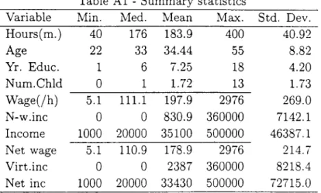
In Table AI in the Appendix, summary statistics of the variables in the sample are presented. 'Hours' are monthly hours in ali jobs. Note that maximum possible hours are (2-1 hours x 7 days in a week x 4 weeks) 672. 'Age' is the age of the employee in the month of the survey. ·Yr. Educ.' is the number of years of education of the respondentlO. 'Num.Chld' is the calculated number of children of the employee.
'vVage' is the hourly wage rate. It is calculated as monthly earnings in ali jobs divided by four times the number of weekly hours in those jobs. 'Non-wage Income' is own nonlabor income. 'Net income' is calculated as the sum of net earnings and virtual income.
5
Empirical results
The labor supply estimates are in Table 1. Note that the Durbin-Hausman-\VU test has a calculated value of 580.27, decisively rejecting the hypothesis that the 2SLS estimates are equal to the OLS parametersl l. This suggests that the net wages are
correlated with the errar term of the hours equation. Only 2SLS and 2SRQ (1\")
results should be used for analysis 12. The net wage and virtual income variables
to avoid a 'tax marriage penalty'.
9The work card is a document where the terms of employment are detailed and is recognized as an indicator of participation in the the formal sector of the economy. li the employer 'signs' the employee's work card, the latter has withholding taxes collected. but also has documentation of work time for retirement purposes and is eligible to receive severance paid ando after 1988. unemployment insurance. As almost all income tax revenues are collected at the source. and the means to evade increase dramatically for those working in the informal (underground) economy. i.e., without work cardo it is assumed that only employees who have a work card pay income taxes.
lar would like to thank David Lam and Suzanne Duryea for suggestions on how to calculate this variable.
llThe first stage wage and in come equation estimates are presented in Ribeiro(1996a). The exogenous variables Zl in the estimating equations are age. years of education. the number of children, and race and region dummies. The set of exogenous variables (instruments) Z also include age squared, number of working family members, a work card dummy. seniority (number of years in the current job), dummies for the sector in which the employee has a job. and occupation dummies. rdentification of the system is guaranteed by assuming that: seniority. occupation. and sector variables appear in the wage equation only; the number of children. onl)" appears in the hours equation; and the number of working family members only appears in the income equation. AIso. \Vhite's (1984) heteroscedasticity consistent covariance matrix was used in the calculations.
"
•
were instrumented by least squares, and are used for both 2SLS and 2SRQ. In the 2SLS results, the wage and income coefficients are negative and signifi-cantly different from zero. On the demographic variables. those older tend to work more. Labor supply hours are also positively related to the education level. And as in most labor supply studies, the number of children increase the labor supply of married men.
The 2SRQ estimates at the 10, 25, 50, 75 and 90th quantiles yield some surprising results. The wage and income variables influence the number of work hours only for those working more than the standard workweek of 40 hours as the conditional
10 and 25th quantile estimates do not depend on the cO\'ariates (note the intercept estimate is 160 hours of work in 4 weeks. or 40 hours a \veek). And it is not the case that the coefficients are estimated with large variance. so that they are insignificam. but that the coefficients themselves are all smaller than 10-5 (10-8 for the virtual income variable), i.e., very small.
[Table 1 about here 1
This suggests that other factors influence the labor supply decision for many individuais. Those agents that considered themseh'es constrained in their hoursjjob choice were excluded from the sample, so it is not the case that outside constraints 'create' preferences for working the standard workweek of 40 hours. For Sweden. it is also the case that the almost totality of agents working the standard workweek are not dissatisfied with the number of hours of work Sacklen (199.5).
For the upper quantiles, the coefficients are all significant and of the same signo They are of the same sign that the 2SLS estimates. also. Their magnitude does change, indicating heterogeneity in the sample. It is seen that the magnitude of parameters increases for longer hours of work.
In the lower part of the table, the obtained parameter values were applied to the elasticity formulae for two 'representative' agents, with mean and median character-istics. Both the mean and median are used because the distribution of wages and demographics is skewed to the left 13.
If one is to interpret the erro r term in the regression model as arising solely from heterogeneity, agents at 10\v quantiles can be interpreted as having weaker preferences for work and those at higher quantiles, high preferences for work. from the definition of regression quantiles. Recall that given the same vector of wages and income, those at high quantiles work longer hours. Alternative, without this
13 As the distributions are asymmetric. there is no 'natural' center of the distributions. i.e .. what
•
•
error restriction, the elasticities calculated at different quantiles can be interpreted as confidence intervals for the 2SLS estimates. This follmvs from the relationship of least squares as providing a conditional point estimate of hours of work and RQ providing interval estimates of this variable .
The most striking result is the range and asymmetry of values for elasticities in the data. For example, the 2SLS (conditional mean) compensated wage elasticity for the median representative agent of .056 varies from O (at the 10% quantile) to .39 (at the 90% percentile). An important consequence of these results under an assumption of heterogeneity error only is that the effects of changes in income and wages will be much more important for those working long hours (those who are at the upper quantiles of the hours distribution) than for those working the standard work week. This is true regardless of the levei of the wage rate. Note that such implication cannot be inferred from conditional mean estimates.
Regarding the other elasticities, the range of estimates across the population. or confidence intervals based on the 10% and 90% quantiles indicate that the wage elasticity for the sample is between -.14 and O and that the income elasticity across quantiles range from -.026 to O.
The asymmetric range of elasticities around the conditional mean, obtained by the RQ estimates indicates that the use of Gaussian errors relies on not always reasonable assumptions. Further, the least squares elasticities are influenced by those working the standard workweek, which were found to have zero wage and income elasticities. On the other hand, by an extremely important property of RQs (and the base for Powell's (1986) censored r€gression quantiles estimator). estimates of the elasticities for those at long hours are not influenced by those workers. Recall that RQs model the order (rank), quantiles, of the regressand not their magnit ude. This property is shared also by robust nonparametric one sample tests. such as the \Vilcoxon test.
It must be pointed out that Hendricks and Koenker (1992) also obtained a com-parable result for the demand of electricity in Chicago. The explanatory \'ariables did not influence the consumption of low (baseload) leveis of electricity, while the peaks in consumption were explained by, say. the number of appliances and people in the household. These very interesting results, completely hidden from researchers using conditional mean estimates, highlight the power of RQ in uncovering the actual form of the variability in responses of the regressors on the conditional distribution of the dependent variable.
6
Conclusion
•
•
urban private sector employees in Brazil. \Ve have also provided previously unknown labor supply elasticities and semiparametric confidence intervals for these estimates. In the estimation procedure, in come taxes and possible endogeneity of the net wage and non-Iabor income variables were considered. Specification tests suggest that those variables were indeed correlated with the error term and thus Two Stage Regression Quantiles (2SRQ) and Two Stage Least Squares (2SLS) were employed . The most surprising result, indicated by 2SRQ estimates, is that the choice of hours for those working the standard workweek of 40 hours is not a function of the variables in the labor supply model, as the estimated coefficients were ali effectively zero. On the other hand, for those v,:orking longe r hours, it was found that the labor supply function is back\vard bending, with the uncompensated wage elasticities ranging from -.06 to -.14. Compensated mean elasticities point estimates for representative agents are of the order of -.10 so that a 10% increase in net wages would lead to an expected 1% decrease in work hours. These results are similar to those surveyed by Pencavel (1986) and for Indonesia (Rochjadi and Leuthold, 1994). The main implications of the above results are that (i) conditional mean es-timates provide only limited information on the conditional distribution of work hours; (ii) the parameters of the conditional work hours distribution are distributed asymmetrically around the mean, so Gaussian based inferences are likely to be mis-leading; and (iii) there seems to be some type of . habi t formation' in the choice of work hours by a vast majority of workers who work the standard workweek. so that wage and nonlabor income changes are likely to affect those working long hours only. The above results provide some interesting implications for the study of labor supply, motivating more research on the topic. It must be said that the model used here is very simple, abstracting from family labor supply effects and response to wage and income changes in other \vays but work hours, such as choice of self-employmenr. or in the case of income taxes, the formal or informal sector. An immediate and important extension would be to study the labor supply of women, as their labor supply has been estimated to be elastic to changes in the v,'age rate, contrary to male labor supply results.
References
Amemiya, T. (1982). Two stage least absolute deviations estimators, Econometrica, 50, 689-711.
Blomquist, S. (1996). Estimation methods for male labor supply functions: how to take into account taxes. Joumal of Econometrics, 70383-405
•
•
•
Brasil, Ministério da Economia (1991). Manual de Ajuste do Imposto de Renda. ano base 1990. Brasflia: Receita Federal.
Buchinsky, ~I. (1994). Changes in the US wage structure 1963-1987: Application of quantile regression. Econometrica. 62, 405-458.
(1995). Estimating the asymptotic covariance matrix for quantile regression models: a Monte Carlo study. Journal of Econometrics. 68, 303-338.
Davidson, R. and MacKinnon, C. (1993). Estimation and Inference in Econometrics.
New York: Oxford University Press.
Hall, P. and Sheather, S.J. (1988). On the distribution of a studentized quantile.
Journal of the Royal Statistical Society. ser. B. 50, 381-391.
Hausman, J. (1981). Labor Supply. in: Aaron, H. and Pechman, J. eds .. How Taxes Affect Economic Activity. Washington D.C.: Brookings.
(1985). Ta..xes and Labor Supply. in A.J. Auerbach and M. Feldstein (eds.),
Handbook of Public Economics, vol I. Amsterdam:North-Holland.
Hendricks W. and Koenker, R. (1992). Hierarchical spline models for conditional quantiles and the demand for electricity. Journal of the A merican Statistical
Association, 87, 58-67.
Jatobá, J. (1994). A famÍlia brasileira na força de trabalho: um estudo de oferta de trabalho - 1978j88.Pesquisa e Planejamento Econômico, 24(1), 1-34.
Killingsworth, M. (1983). Labor Supply. New York:Cambridge University.
Koenker. R. (1994). Confidence intervals for regression quantiles. m: .~.1andl. P. and Huskova, M., eds., Asymptotic Statistics. Proceedings of the 5th Prague Conference.
Koenker R. and Bassett, C. (1978). Regression quantiles. Econometrica, 46, 33-50. - (1982). Robust tests for heteroscedasticity based on regression quantiles.
Econo-metrica. 50, 43-61.
Koenker. R. and d'Orey, V. (1994). A remark on computing regression quantiles.
Applied Statistics, 36, 383-393.
Maddala, C.S. (1974). Some small sample evidence on tests of significance in simul-taneous equations models. Econometrica, 42, 841-851.
•
•
•
Moffitt, R. (1990). Special issue on taxation and labor supply in industrialized
countriesed.Journal of Human Resources, 25, vo1.3, Summer.
?vIroz, T. (1987). The sensitivity of an empirical model of married v"omen's hours of work to economic and statistical assumptions. Econometrica. 55, 765-799.
Pencavel, J. (1986). Labor supply of men: a survey. in. Ashenfelter. Q. and Layard . R., (eds.) Handbook of Labor Economics. v.l. Amsterdam: North- Holland. Powell, J. (1983). The asymptotic normality of two-stage least absolute deviations
estimator. Econometrica. 51, 1569-1575.
- (1986). Censored regression quantiles. Journal of Econometrics. 32, 143-15·5.
Ribeiro, E.P. (1996a). The Effect of Personal Income Taxes on Labor Supp/y In
Brazü: an application of quantile regression. Umpublished Ph.D. thesis. Uni-versity of Illinois at Urbana-Champaign.
Ribeiro, E.P. (1996b). Small sample evidence of regression quantile estimates for structural models: estimation and testing. Anais do XVIII Encontro Brasileiro de Econometria, v.2. Águas de Lindóia, SP: SBE
Rochjadi, A. and Leuthold, J.H.(1994). The effect of taxation on labor supply in a Developing country: evidence from cross-sectional data. Economic
Deve/op-ment and Cultural Change, 42, 333-350.
Rosen, H.S. (1978). The measurement of excess burden with explicit utility func-tions. Journal of Political Economy, 86, S121-S135.
Sacklen. H. (1995). Labor supply, income taxes and hours constraints in Sweden.
Dept. of Economics Working Paper 95:2. University of Uppsala.
Triest, R. (1990) The effect of income taxation on labor supply in the United States.
Journal of Human Resources, 25, 491-516.
•
•
Table 1: Labor supply estimates using 2SLS and 2SRQ.Variable rq( .1) rq( .25) rq(.5) rq(.75) rq( .9) 2SLS
l/w .0011 .0012 -284.3 -769.9 -4606 -943.3
O O (15.80) (26.24) (ll3.6) (107.6)
vy/w 0.0 0.0 -.1231 -.1245 -.4329 -.1·500
O O (.0037) (.0063) (.0271) (.0184)
Age/w 0.0 0.0 36.ll 44.68 138.1 44.77
O O (1.040) (1.729) (7.487) (2.86)
Yr.Educ/w 0.0 0.0 171.8 155.6 381.9 141.9
O O (6.489) (10.78) ( 46.67) (7.55)
Num.Chld/w 0.0 0.0 120.1 155.7 341.9 142.3
O O (7.106) (11.80) (51.ll) (14.58)
lnt. 160.0 160.0 155.3 175.3 201.9 168.2
O O (.5015) (.8330) (3.607) ( .054)
cor(h, h), .061 .130 .285 .287 .242 .226
~1AE 29.56 29.01 26.83 32.70 63.64 27.98 Source: PNAD 1990 data. Notes: n=24,733;
t:
p-value> .05;Region and Race dummies not shown; s.e. in brackets.
2SLS and 2SRQ Labor supply estimates elasticities at mean and median
Variable rq( .1) rq(.25) rq(.5) rq(.75) rq(.9) 2SLS
LES :YIodel - mean agent
\Vage 0.0 0.0 -.072 -.060 -.079 -.051
lncome 0.0 0.0 -.010 -.009 -.026 -.Oll
Comp. 0.0 0.0 .051 .064 .35 .098
LES Model - median agent
Wage 0.0 0.0 -.120 -.099 -.14 -.093
lncome 0.0 0.0 0.0 0.0 0.0 0.0
•
Table A1 - Summary statistics
Variable Min. Med. Mean Max. Std. Dev.
Hours(m.) 40 176 183.9 400 40.92
Age 22 33 34.44 55 8.82
Yr. Educ. 1 6 7.25 18 4.20
Num.Chld O 1 1.72 13 1.73
Wage(jh) 5.1 111.1 197.9 2976 269.0
N-w.inc O O 830.9 360000 7142.1
Income 1000 20000 35100 500000 46387.1 Net wage 5.1 110.9 178.9 2976 214.7
Virt.inc O O 2387 360000 8218.4
"".Cham. P/EPGE SPE R484c Autor Ribclro, Eduardo Pontual.
Título ('onditlonal labour supply. quantile functions In
1111111111111111111111111111111111111111
089653 52434