Markups’ Cyclical Behavior: The role of Demand and Supply Shocks

(1)

António Afonso & João Tovar Jalles

Markups’ Cyclical Behavior: The role of

Demand and Supply Shocks

WP08/2015/DE/UECE

_________________________________________________________

De pa rtme nt o f Ec o no mic s

W

ORKING

P

APERS

(2)

Markups’ Cyclical Behavior: The role of Demand and

Supply Shocks

*

February 2015

António Afonso

$

and João Tovar Jalles



Abstract

We assess how demand and supply shocks (identified via the Blanchard and Quah (1989) SVAR approach) in 14 OECD countries affect mark-ups. We find that individual responses of markups to demand shocks push down the markup for most countries (confirmed in the panel analysis). On the other hand, a supply shock has a more mixed effect.

JEL: C23, E32, E62

Keywords: Blanchard-Quah, mark-up, VAR, impulse response function, local projection

1. INTRODUCTION

The interaction between fiscal policy effectiveness and imperfect competition has received some attention in economic theory (Hall 2009; Christiano et al. 2011; and Woodford 2011; and the survey by Costa and Dixon, 2011). In particular, the cyclical behavior of markups following government spending shocks has been closely analyzed. The New Keynesian Synthesis have developed models that produce undesired endogenous markups due to nominal rigidity, enhancing the effectiveness of demand-side policy, including fiscal policy. Moreover, macroeconomic models with time-varying desired markups are even more attractive as they work similarly to productivity shocks in the presence of active fiscal policy (Ravn et al., 2006).

*

The opinions expressed herein are those of the authors. The usual disclaimer applies. $

ISEG/UL - University of Lisbon, Department of Economics; UECE – Research Unit on Complexity and Economics. UECE is supported by FCT (Fundação para a Ciência e a Tecnologia, Portugal), email: [email protected].



(3)

2 The theoretical literature on endogenous markups is dominated by the view that markups behave counter-cyclically following a demand shock. Indeed, when a positive shock originates in the demand side, the marginal cost function is only indirectly affected and the main effect depends on how the individual demand function responds (see e.g. Gali, 1994; Goodfriend and King, 1997; Clarida et al. 1999; Ravn et al., 2006). However, with a positive supply shock, we expect marginal costs to decrease for a given output. Therefore, assuming that the indirect effect on prices via demand is small, markups tend to increase implying a pro-cyclical average markup.

Several papers that try to measure markups for different industries over a period find evidence of a mildly counter-cyclical behavior (Rotemberg and Woodford, 1999; Martins and Scarpetta, 2002), with Afonso and Costa (2013) reporting that markups are pro-cyclical with productivity and counter-cyclical government spending. The combination of demand and supply shocks is a possible explanation for the existing evidence on counter-cyclicality.

We contribute to this literature by looking at how demand and supply shocks in 14 OECD countries affect the evolution of markups in the short to medium run. The two types of shocks are decomposed via the Blanchard and Quah (1989) (BQ) methodology based on a SVAR identification. We conduct both individual country analyses and a panel assessment.

Our results show that individual responses of the markups to demand shocks show that a demand shock pushes down the markup for most countries (confirmed in panel analysis). On the other hand, a supply shock has a more mixed effect.

2. METHODOLOGY

The market is the price wedge

𝜇𝑖𝑡 =_𝑀𝐶𝑃𝑖𝑡_𝑖𝑡 (1)

where 𝑃_𝑖𝑡 represents the price of the good produced by firm i and 𝑀𝐶_𝑖𝑡 stands for its marginal cost, in

t.

Since marginal costs are not observable, one can estimate them using the relationship 𝑀𝐶_𝑖𝑡 = 𝑊𝑡/𝑀𝑃𝐿𝑖𝑡 where 𝑊𝑡 is the nominal wage rate (assuming homogeneous labor input) and 𝑀𝑃𝐿𝑖𝑡 is the

(4)

3 In order to separate demand from supply shocks we follow Blanchard and Quah (1989) approach applied to real GDP and unemployment rate data in quarterly frequency between 1970 and 2007. The resulting quarterly series for the shocks are then converted into annual frequency in order to match the markup series.

Under the Blanchard-Quah decomposition, consider the following bivariate SVAR model:

𝐴0𝑋𝑡 = 𝐴1(𝐿)𝑋𝑡+ 𝐵𝜀𝑡 (2)

where 𝑋_𝑡 = (∆𝑦_𝑡, ∆𝑢_𝑡) and y and u are measures of real output and unemployment, respectively.1 Here 𝜀_𝑡 = (𝜀_𝑡𝑠, 𝜀_𝑡𝑑) with 𝜀_𝑡𝑠 and 𝜀_𝑡𝑑 being one standard deviation supply and demand shocks, respectively. 𝐴₀ is a 2x2 matrix, 𝐴₁(𝐿) = ∑ 𝐴𝑞_𝑖=1 _1𝑖𝐿𝑖 shoes matrices of lag coefficients of the SVAR system. The BQ approach assumes that two shocks are not correlated, and hence, B is a diagonal matrix. Denote the diagonal elements (essentially are the standard deviations of the two shocks) in B by 𝑏₁₁ and 𝑏₁₂.

The structural shocks in Equation (1) are not directly observable. It is the usual practice to estimate the reduced form VAR and use the estimated parameters and residuals in the reduced form VAR to retrieve the structural shocks. The reduced form VAR has the form:

𝑋𝑡 = 𝐶(𝐿)𝑋𝑡+ 𝑒𝑡 (3)

with 𝐶(𝐿) = ∑𝑞_𝑖=1𝐶_𝑖𝐿𝑖 being the matrices of estimated lag coefficients and 𝑒_𝑡being the vector of two residual series. Equivalently, this reduced form VAR can be expressed in more simple way as:

∆𝑦𝑡 = ∑𝑞𝑖=1𝑐11𝑖 ∆𝑦𝑡−1+ ∑𝑞𝑖=1𝑐12𝑖 ∆𝑢𝑡−1+ 𝑒𝑡𝑦 (4)

∆𝑢𝑡= ∑𝑞𝑖=1𝑐21𝑖 ∆𝑢𝑡−1+ ∑𝑞𝑖=1𝑐22𝑖 ∆𝑦𝑡−1+ 𝑒𝑡𝑢

The relation between the structural shocks and the reduced form VAR residuals is crucial in identifying the structural shocks. This can be expressed as:

𝑒𝑡 = 𝐺0𝜀𝑡 (5)

Where 𝐺₀ = 𝐴−1₀ 𝐵 is a 2x2 matrix representing the contemporaneous effects of the one standard deviation shocks on the two variables.

It follows that one cannot make a distinction between the supply and demand equations unless we impose some qualifications for defining the shocks. In order to separate out the demand from the

1

(5)

4 supply shocks, the BQ method defines a demand shock as the one that does not have any long run effect on the output level. If we denote 𝐺₀ as:

𝐺0 = [𝑔11

0 _𝑔

120

𝑔210 𝑔220 ]

(6) Then the long run restriction essentially implies that:

𝑔120 = − ∑ 𝑐12

𝑖 𝑖

1−∑ 𝑐𝑖 ₂₂𝑖 𝑔22

0 ₍₇₎

Imposition of this restriction makes the SVAR system exactly identified and one can now identify the structural shocks 𝜀_𝑡𝑠 and 𝜀_𝑡𝑑 by using the information from the estimated reduced form VAR.

3. RESULTS

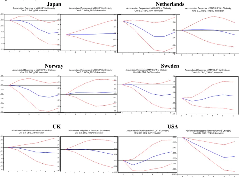
Looking at Figure 1, the individual responses of the markup to demand shocks show that a demand shock pushes down the markup for all countries, except in the case of Finland, in the short run, and in the case of Denmark, where the effect is negligible. On the other hand, a supply shock has a more mixed effect, increasing the markup in Belgium, France and Italy, but decreasing it in the first two-three quarters in Denmark, Sweden, and US.

[Figure 1]

To estimate the panel impact of demand and supply shocks on the evolution of markups over the short and medium-run, we follow the method proposed by Jorda (2005) which consists of estimating impulse response functions (IRFs) directly from local projections. For each period k the following equation is estimated on annual data:

𝑌𝑖,𝑡+𝑘− 𝑌𝑖,𝑡 = 𝛼𝑖𝑘+ 𝑇𝑖𝑚𝑒𝑡𝑘+ ∑𝑗=1𝑙 𝛾𝑗𝑘∆𝑌𝑖,𝑡−𝑗+ 𝛽𝑘𝑆𝑖,𝑡+ 𝜀𝑖,𝑡𝑘 (8)

(6)

5 Impulse response functions are obtained by plotting the estimated 𝛽_𝑘 for k= 1,…,6, with confidence bands computed using the standard deviations of the estimated coefficients.2

An alternative way of estimating the dynamic impact of demand and supply shocks is to estimate an ARDL equation of changes in the markup and demand and supply shocks and to compute the IRFs from the estimated coefficients (Cerra and Saxena, 2008). However, the IRFs derived using this approach tend to be sensitive to the choice of the number of lags this making the IRFs potentially unstable. In addition, the significance of long-lasting effects with ARDL models can be simply driven by the use of one-type-of-shock models (Cai and Den Haan, 2009). This is particularly true when the dependent variable is highly persistent, as in our analysis. In contrast, the approach used here does not suffer from these problems because the coefficients associated with the lags of the change in the dependent variable enter only as control variables and are not used to derive the IRFs, and since the structure of the equation does not impose permanent effects.

Finally, confidence bands associated with the estimated IRFs are easily computed using the standard deviations of the estimated coefficients and Montecarlo simulations are not required.

[Figure 2]

In Figure 2 we can observe, and distinctly confirm, that for the panel as a whole there is a statistically significant negative impact of demand shocks on mark-ups that extends up to six quarters. On the other hand, the markup also reacts to a supply shock, although the result, in this case, is much less precisely estimated. Once again, our findings are broadly in line with previous studies. Finally, results were subjected to several robustness checks.3

4. CONCLUSION

We have assessed the effect on markups of demand and supply shocks in OECD countries using a SVAR identification. Our results show that the responses of the markups to demand shocks show are

2

While the presence of a lagged dependent variable and country fixed effects may in principle bias the estimation of 𝛾_𝑗𝑘 and

𝛽𝑘in small samples (Nickell, 1981), the length of the time dimension mitigates this concern. The finite sample bias is in order of 1/T, where T in our sample is 38.

3

(7)

6 negative, pushing down the markup for most countries (which we also confirmed in a panel). On the other hand, a supply shock has a more mixed effect on the markup, being also more negative in the case of the panel analysis. Such effects via demand and supply shocks are a potential explanation for the counter-cyclicality of markups found in the literature.

REFERENCES

1. Afonso, A., Costa, L. (2013), “Market Power and Fiscal Policy in OECD countries”, Applied Economics, 45 (32), 4545-4555.

2. Blanchard, O. and D. Quah. (1989), “The dynamic effects of aggregate demand and supply disturbances”, American Economic Review 79, 655-673.

3. Cai, X., and W. J. Den Haan. (2009), “Predicting Recoveries and the Importance of Using Enough

Information”, CEPR Discussion Paper No. 7508.

4. Cerra, V., and S. Saxena. (2008), “Growth Dynamics: The Myth of Economic Recovery,” American Economic Review, 98(1), 439-57.

5. Christiano, L., M. Eichenbaum, and S. Rebelo. (2011), “When is the Government Spending Multiplier

Large?” Journal of Political Economy, 119(1), 78-121.

6. Clarida, R., Galí, J. and Gertler, M. (1999), “The Science of Monetary Policy: A New Keynesian Perspective”. Journal of Economic Literature, 37, 1661-1707.

7. Costa, L. and Dixon, H. D. (2011), “Fiscal policy under imperfect competition with flexible prices: An overview and survey”. Economics: The Open-Access, Open Assessment E-Journal, 5(3).

8. Galí, J. (1994), “Monopolistic Competition, Endogenous Markups, and Growth”. European Economic Review, 38(3-4), 748-756.

9. Goodfriend, M. and King, R. (1997), “The New Neo-Classical Synthesis and the Role of Monetary Policy”. NBER Macroeconomics Annual 231-283.

10. Hall, R. (2009), “By How Much Does GDP Rise If the Government Buys More Output?”. NBER Working Papers 15496.

11. Jorda, O. (2005), “Estimation and Inference of Impulse Responses by Local Projections,” American Economic Review, 95(1), 161–82.

12. Martins, J.O. and Scarpetta, S. (2002), “Estimation of the Cyclical Behaviour of Mark-ups: A technical note”. OECD Economic Studies 34(1), 173-188.

13. Nickell, S. (1981), “Biases in dynamic models with fixed effects”, Econometrica, 49, 1417–1426. 14. Ravn, M., Schmitt-Grohé, S., and Uribe, M. (2006), “Deep habits”. Review of Economic Studies, 73(1), 195–218

15. Rotemberg, J. and Woodford, M. (1999), “The Cyclical Behavior of Prices and Costs”. In: Taylor, J. and Woodford, M., (Eds.) Handbook of Macroeconomics, Elsevier, Amsterdam, 1051-1135.

(8)

7

Figure 1. Individual Responses of Markup to Demand and Supply Shocks

Australia Belgium

-.03 -.02 -.01 .00 .01 .02

1 2 3 4 5 6

Accumulated Response of MARKUP1 to Cholesky One S.D. DBQ_GAP Innovation

-.03 -.02 -.01 .00 .01 .02

1 2 3 4 5 6

Accumulated Response of MARKUP1 to Cholesky One S.D. DBQ_TREND Innovation

-.020 -.016 -.012 -.008 -.004 .000 .004

1 2 3 4 5 6

-.010 -.005 .000 .005 .010 .015 .020 .025 .030

1 2 3 4 5 6

Canada Denmark

-.030 -.025 -.020 -.015 -.010 -.005 .000 .005

1 2 3 4 5 6

-.020 -.016 -.012 -.008 -.004 .000 .004 .008 .012 .016

1 2 3 4 5 6

-.028 -.024 -.020 -.016 -.012 -.008 -.004 .000 .004 .008 .012

1 2 3 4 5 6

-.03 -.02 -.01 .00 .01 .02

1 2 3 4 5 6

Finland France

-.07 -.06 -.05 -.04 -.03 -.02 -.01 .00 .01 .02

1 2 3 4 5 6

-.02 -.01 .00 .01 .02 .03 .04 .05 .06

1 2 3 4 5 6

-.05 -.04 -.03 -.02 -.01 .00 .01

1 2 3 4 5 6

-.008 -.004 .000 .004 .008 .012 .016 .020 .024 .028 .032

1 2 3 4 5 6

Germany Italy

-.025 -.020 -.015 -.010 -.005 .000 .005 .010

1 2 3 4 5 6

-.020 -.015 -.010 -.005 .000 .005 .010 .015 .020

1 2 3 4 5 6

-.07 -.06 -.05 -.04 -.03 -.02 -.01 .00 .01

1 2 3 4 5 6

-.03 -.02 -.01 .00 .01 .02 .03 .04 .05 .06

1 2 3 4 5 6

(9)

8

Figure 1. (cont.)

Japan Netherlands

-.025 -.020 -.015 -.010 -.005 .000 .005

1 2 3 4 5 6

-.03 -.02 -.01 .00 .01 .02 .03 .04

1 2 3 4 5 6

-.05 -.04 -.03 -.02 -.01 .00 .01

1 2 3 4 5 6

-.03 -.02 -.01 .00 .01 .02

1 2 3 4 5 6

Norway Sweden

-.06 -.05 -.04 -.03 -.02 -.01 .00 .01 .02

1 2 3 4 5 6

-.06 -.04 -.02 .00 .02 .04 .06

1 2 3 4 5 6

-.06 -.05 -.04 -.03 -.02 -.01 .00 .01 .02

1 2 3 4 5 6

-.03 -.02 -.01 .00 .01 .02 .03 .04

1 2 3 4 5 6

UK USA

-.06 -.05 -.04 -.03 -.02 -.01 .00 .01 .02 .03

1 2 3 4 5 6

-.05 -.04 -.03 -.02 -.01 .00 .01 .02 .03

1 2 3 4 5 6

-.008 -.004 .000 .004 .008 .012 .016

1 2 3 4 5 6

-.035 -.030 -.025 -.020 -.015 -.010 -.005 .000

1 2 3 4 5 6

Note: Responses to a one-standard deviation shock. For each country, the left (right) char represents the impulse of mark-ups to demand (supply) shocks.

Figure 2. Panel Responses of Markup to Demand and Supply Shocks-Local Projection Estimator

Demand Shocks Supply Shocks

Note: Dotted lines equal one standard error confidence bands. See main text for further details.

-0.9 -0.8 -0.7 -0.6 -0.5 -0.4 -0.3 -0.2 -0.1 0

0 1 2 3 4 5 6

estimate lower limit upper limit

-0.6 -0.5 -0.4 -0.3 -0.2 -0.1 0 0.1

0 1 2 3 4 5 6