, ,
J
...
..
:. -MBセMG@P/EPGE
SA
T342p
FUNDAÇÃO GETULIO VARGAS
セT@
FGV
EPGE
SEMINÁRIOS DE ALMOÇO
DA EPGE
lhe power of the purse: What do the
data say on US federal budget
allocation to the states ?
CECILIA TESTA
(University of London)
Data: 13/08/2004 (Sexta-feira)
Horário:12h 30min
Local:
Praia de Botafogo, 190 - 110 andar
Auditório nO 1
Coordenação:
,..
The power of the purse: what do the data say on US
federal budget allocation to the states?*
Valentino Larcineset Leonzio Rizzo+and Cecilia Testa§
June 2004
(preliminary draft, all comments welcome)
Abstract
This paper provides new evidence on the determinants of the allocation of the US federal budget to the states and tests the capability of congressional, electoral and par-tisan theories to explain such allocation. We find that socio-economic characteristics are important explanatory variables but are not sufficient to explain the disparities in the distribution of federal monies. First, prestige committee membership is not con-ducive to pork-barrelling. We do not find any evidence that marginal states receive more funding; on the opposite, safe states tend to be rewarded. Also, states that are historically "swing" in presidential elections tend to receive more funds. Finally, we find strong evidence supporting partisan theories of budget allocation. States whose governor has the same political affiliation of the President receive more federal funds; while states whose representatives belong to a majority opposing the president party receive less funds.
·We wish to thank Tim Besley and Jim Snyder for helpful discussions and the participants to the STICERD work in progress seminar, the Royal Holloway internai seminar and the Ente Einaudi seminar, the University of Sao Paulo Applied Microconomics Semaninar series, for useful comments and suggestions. Remaining errors are only ours.
tDepartment of Goverment and STICERD London School of Economics and Political Science. email: v [email protected]
+Universita' di Ferrara and STICERD (LSE). Email:[email protected]
•
"No money shall be drawn from the Treasury but in Consequence of Appropriations made by law" US Constitution, article I, Section 9, Clause 7.
1.
Introduction
The allocation of the federal budget in the United States is the outcome of a complex pro-cess involving numerous institutionalplayers. A vast theoretical and empírical líterature has devoted a formidable effort to the study of this process, but from an empirical perspec-tive, the results of such efforts are much more questionable1 . For example, if we look for an assessment on the relative power of the President versus the Congress, or on whether individual Committee members are more infiuential than Political Parties, we would sur-prisingly realize that the existing literature only provides some partial insights. Hence, the main goal of this paper is to carry out a new empirical study re-assessing the infiuence of the many institutional players in the budget allocation to establish who has ultimately the power of the purse in the allocation of US federal monies and how this power affects the distribution of federal funds across states. Importantly, most existing studies seem to assume that pork barreI polítics is a prerogative of the Congress2, while the role of the President has been substantially neglected3 , and the infiuence of polítical parties has not been extensively analyzed4 . This paper will provide new evidence on the crucial role played by both President and Polítical Parties, showing that they have substantial, if not greater power than Congress in the allocation of the federal budget.
From a methodological standpoint, the main advantage of our analysis is that, differently from previous empirical studies, which have considered either a cross section or a very short time dimension, we use panel data for a relatively long time span. This allows us to test several theories by using the same dataset, whilst isolating state and year fixed effects from our variables of interest. The existing studies are, in fact, hardly comparable because they tend to focus on different spending programs for some specific years. As a consequence it is difficult to say if what we learn is merely due to particular features of the data considered, rather than to proper and long lasting polítical features of the political
1 For an overview on the theoretical and empirical liteture, see the next section related literature. 2See, for example, Owens and Wade (1984).
3Studies on New Deal spending are the only exception. For an overview see Couch and Shugarth (1998). 4See Snyder and Levitt (1997) .
processo Hence, thanks to the panel dimension, our estimates provide comparable results on the predictive power of alternative theories. Furthermore, by simultaneously estimating in the same regressions the impact of all the various channels of political influence, we address the issue of the omitted variable bias that is likely to affect previous studies, thereby improving on the robustness of our findings.
To briefly summarize our main result, we find that the President has a large influence on budget allocation to the states. In particular, states that are ideologically leaning with the President, i.e. states with high share of presidential vote or with a governor belonging to the same party of the President, tend to be rewarded with more funds. On the other hand, states with close presidential race do not receive more money, nor do states who swung in the most recent election. However, we find evidence of spending being targeted to states that, over a long time period, have been observed swinging frequently. Hence, overall our analysis suggest that the President is a very influential player as he may be able to direct more funding toward states that are run by "friendly" governors, have large groups of "core supporters" , and are traditionally "swíng" in the presidential election. We find less support ín favor of congressional theories. In particular, having representatives in prestige committees (with the partial exceptíon ofthe committee for ways and means) does not seem to provide any financiaI advantage to states.
The remainder of the paper is organized as follows. In section 2 we provide an overview of the theoretical literature from which we derive the main predictions that we will sub-sequently test with our data. Section 3 describes our dataset and lays out our empirical approach. Section 4 presents our main results and sectíon 5 summarizes and concludes.
2. Theories of budget allocation
A large theoretical líterature that has attempted to dísentangle the determínants of fed-eral budget allocatíon from dífferent angles. Accordíng to standard welfare economícs, the distríbutíon of federal funds should only depend on the preferences of a benevolent social planner, and therefore resources should be allocated to dífferent states only accordíng to theír needs. In empirical terms, this distributíon should be fully captured by economic and demographic variables. This useful normatíve benchmark ís often at odds with stylized facts and hardly recognized as a reliable posítive theory of budget allocation. Among the firsts .. to point out the limíts of welfare economícs as a posítíve theory is the work of Nískanen
),
..
(1971), who stresses the incentives of bureaucrats to maximize their available budget (see also Gilberst and Specht, 1974, and Arnold, 1981). However, no convincing evidence have been found to support this view (Stein, 1981). An alternative vast stream of literature focuses on Congress, stressing the prominence of individual representatives on the budget allocation. Finally, the literature on party politics points out that political parties may be influential organizations that ultimately are more relevant than individual representatives in determining federal budget allocation.
These different theoretical approaches clearly identify the key players in the budget pro-cess, but which player is eventually the most influential and why, is ultimately an empirical question that we try to address in this paper. Hence, in what follows, we briefly summarize the main results of the literature, highlighting the theoretical hypotheses that will provide the basic structure of our empirical analysis.
2.1. Congressional theories
The congressional theories of the budget process emphasize the role played by congressional actors (Bailey and Samuel 1952, Fenno 1973, Kiewiet and McCubbins 1988). Individual representatives occupying key positions in the budget process or belonging to some prestige committee can be able to convey a disproportionate amount of money to their districts. Logrolling across the representatives or Committee members of different districts or states (and rather independently of party lines) is in this case the determinant of the distribution of the budget. Most studies in this line of research have focussed on the role of committees as they occupy key positions in the budget allocation process, because they have an advantage both in terms of their agenda setting power (McKelvey and Ordeshook, 1980) and in terms of information and competence (Krehbiel, 1991). Weingast and Marshall (1988) argue that committees are exactly the devices that make logrolling work, by facilitating the trade of influence in the absence of a spot market for exchanging support. Hence, a key prediction of congressional theories is that a disproportionate amount of federal monies should be di-verted towards states that have representatives in influential committees. Consequently, the vast majority of empirical studies on US federal budget allocation focuses on the commit-tee influence in the budget allocation5 . In particular, Owens and Wade (1984) find that
5 Among the numerous studies on committees see Plott (1968), Goss (1972), Ferejohn (1974), Ritt (1976),
Rundquist (1978), Strom (1975), Arnold (1978), Ray (1980), Kiel and McKinzie (1983), Wilson (1986),
i
..
the districts with representatives controlling the chairs of relevant committees receive dis-proportionately more money6. Along the same lines, a more recent study by Alvarez and Saving (1997) shows that the district bias is strong for the Ways and Means committee and stronger in formulaic programs.
2.2. Partisan theories
Alternative theories describing the budget process point out that poliiical parties may ulti-mately have an important impact on congressional activities. Among partizan theories, it is possible to distinguish between two alternative mechanisms of influence. The first one, very common in economic mo deIs and particularly stressed by Lindbeck and Weibull (1987 and 1993) and Dixit and Londregan (1996) points to the presence of electoral bias: funds should be allocated disproportionately to marginal and swing states in order to increase the chance of re-election. An alternative possibility proposed by Cox and McCubbins (1986) points instead to the ideological relationship between voters and candidates. In this case, more funds should be allocated where policy-makers have larger support. Politicalleaders might also want to reinforce or protect their electors share on ideological grounds, and therefore treat party reputation as a public good for individual party members (Cox and McCub-bins,1993). In this case cooperation among representatives is needed in order to increase the chances of re-election or simply to bring bacon at home. Cooperation along party lines (rather than logrolling across representatives) should therefore be expected. Bringing this theory to the data, we should expect that party alignment among different leveIs of govern-ment (for example the president and the state governors) affects the distribution of federal monies. In the context of American politics, the presidential election and the party affilia-tion of the President provide a sensible ground to test these competing theories, since the
Rich (1989), Anderson and Tollison (1991), Owens and Wade (1984), Alvarez and Saving (1997).
GOne interpretation of those results is that committee members alIo cate preferentialIy money to their districts. However, an alternative theory that may as well explain those empirical findings, is that districts with economic interests covered by some programs have members sitting in related committees precisely because those activities are important to the district. Therefore, the disproportion in the alIocation of funds is not due to pork-barrel, but is a consequence of state characteristics (recruitment theory). Indeed the fact that general spending is not affected by committee membership, seems to suggest that the recruitment theory could be a valid explanation for the peculiar pattern of specific programs. In any case, beyond the specific motivations, it is important to understand whether committee members have in fact the power to distort the alIocation of spending towards their preferred destinations and this study seems to show that often they do .
•
winner-takes-it-all electoral vote system should reinforce any sort of bias. Hence, assuming that the president has enough influence on the allocation process ((Kiewiet and Krehbiel (2000))1, we should observe that the characteristics of the presidential race at state leveI and the political alignment of the President with different state government representatives, should affect the allocation of the budget, Le. more funds should go either to the states with close presidential race (marginality and swing bias), or to the states where the incumbent president has received a higher share of votes (ideological bias) and to the states whose gov-ernor and/or other state representatives are politically aligned with the president (partisan alignment) .
The empiricalliterature on partisan budgeting is rather scant. Snyder and Levitt (1995) is one of the few studies that explicitly focuses on the estimation of party influence in the US federal budget allocation8 finding that when congress was dominated by democratic
majorities, outlays at district leveI are positively correlated with the district share of demo-cratic vote9. Concerning presidential elections, with the exception of studies on New Deal spending10 , there are no more general and systematic empirical investigations on presiden-tial influence. Interestingly, the literature on New Deal spending provides support toward both swing and ideological bias (Anderson and Tollison (1991), Couch and Shughart (1998), Fleck (2001a), Fishback et aI (2002), Wallis (1987) and Wright (1974)).
3. Data and methodology
Following the theoretical literature, the hypotheses we want to test may be summarized as follows:
H1: committee members influence the distribution of federal spending to the states (committee influence);
7For an overview on the strugle of power between the President and the Congress, see Oppenheimer (1983).
8Some recent literature has investigated the role of parties in the budget allocation in other countries. Dasgupta et al. (2001) find that lndian states ruled by the same party of the central goverment receive more grants, while Dahlberg and Johansson (2000) find that Swedish regions that are "swing" in the national elections received more of a specific transfer programo
9Evidence of a bias in favour of democratic districts is also reported in the already mentioned works by Owens and Wade (1984) and Alvarez and Saving (1997).
lOFor an overview on New Deal spending literature see Couch and Shughart (1998) and Fishback et ali (2002).
"
•
H2: funds are disproportionately targeted to marginal and swing states in presidential elections (marginality and swing bias);
H3: funds are disproportionately targeted to states that are "safe" in the presidential election (ideological bias);
H4: party alignment between players in different institutional positions increases the receipt of federal funds (party alignment).
We will use data on the 48 US continental States from 1982 to 200011 . Most variables are taken from the Statistical Abstract of the United States, including the spending ag-gregates and information on the economic and demographic characteristics of each state. Some electoral variables are also taken from the Statistical Abstract, including presidentiaI election results, turnout, and data on gubernatorial elections. This dataset has then been compIemented with information from the Offieial Congressional Directory, which has been espeeially usefuI to gather information on committee membership and thus construct the relative variabIes.
Our first step will be to analyze the impact of economic and demographic variables on the allocation of federal expenditure to the states and estimate therefore the following equation:
FEDEXPst
(3.1)
s 1, .. .48;
t
=
1982, ... 2000;where FEDEXPst is real per-capita federal expenditure (outlays) in state s at time
t.
As for all subsequent regressions, we aIways include state fixed effects and year dummies.
Zst is a vector including real income per capita (P Rincome), state population (stpop), unemployment rate (unemp), percentage of eitizens aged 65 or above (aged) and percentage of eitizens between 5 and 17 year old (kids). In all subsequent regressions we will always include these expIanatory variabIes as standard economic and demographic controIs.
We will then augment this basic model with the new explanatory variables that are necessary to test specific theories, estimating an equation of the form:
(3.2)
11 As customary, Alaska, District of Columbia and Hawaii have been excluded.
•
where
P:
w represents the particular set of institutional and political variables under con-sideration. It is impartant to point out that in the US budget allocation process there is a lag between the appropriation of federal funds and the moment when funds are actually spent. This is relevant when estimating the effect of particular institutional and political variables, since current federal outlays have normally been appropriated in past budgetary years. Delays should therefore be taken into account by introducing lagged values forP:
w ' since past policy makers are responsible for current outlays. Furthermore, delays vary according to spending categories. Hence, to give the right weight to lagged independent variables explaining current outlays, we will use weighted averages of laggedP:,
where the weights are determined by the spendout rates usually utilized in official forecasts for each spending categoryl2. Hence, for the aggregate federal expenditure, knowing that approx-imately 60% of funds are spent within one year and assuming that the rest is spent two years later, we regress outlays at timet
on the weighted average of two lagged variables, i.e. P:w=
0.6*
P:t -I+
0.4*
P:t -2 . If instead we consider defense spending, having afirst year spendout rate equal to 67% we get
P:
w=
0.67*
P:
t - I+
0.33*
F;t-2' For directpayments to individuaIs, almost entirely spent within the first year, we have P:w
=
P;t-I . Finally, for grants ,whose composition tend to mirro r the overall federal spending we haveP;w
=
0.6*P;t_1 +0.4*P:t_2 · Other weights have been considered (going backwards up to 5years) but with little noticeable variations in the results as compared to the ones we reporto We begin our analysis by testing hypothesis 1, i.e. considering the role of committee membership. We focus on the most influential committees in the budget process by con-sidering as explanatory variables the number of members by state in the Appropriation, Budget, Ways and Means and Rules committees of the House. If committees are influential players in the overall budget allocation process then we would expect some or all of the co-efficients in the vectar OI to be significantly positive. Besides aggregate federal expenditure, we will also consider selected spending aggregates and estimate equations of the form
(3.3)
12For example, only 11% of procurement is spent within one year and it often takes up to 10 years to completely utilize the resources. This makes procurement a rather unreliable measure if one wants to study political infiuence over outlays using yearly data. For this reason, instead of procurement we prefer to use defense spending in our program-by-program regressions.
•
where j is equal respectively to defense spending, grants, and direct payments to in-dividuaIs (alI in real and per-capita terms). In the case of defense spending we will also include the armed services committee of the Rouse in Psw •
We will subsequently consider the role of electoral competition and test hypotheses 2 and 3. Rence we compare the relative impact of the closeness of presidential elections in each state (presclose) with that of the share of votes obtained by the president in the last election (pres_share). A negative sign of presclose should be regarded as support for the idea that the president tend to direct resources to marginal states in order to increase his chances of re-election, while a positive sign of pres_share can be seen as evidence that incumbents tend to reward ideologícalIy affine states that show their support in elections. In separate regressions, we also take into account the fact that not alI states have the same weight in presidential elections by including the number of electoral votes by state, both in absolute value (elvotes) and per capita (elvotesPC).
Rowever, past closeness is not necessarily the best measure to identify swing states. For this purpose we construct two other variables. The first (swing_state) is a dummy variable equal to one for states that switched their support from one party to the other in the last election. The second (swing_tot) is a time invariant state variable given by the ratio between the overalI number of such changes in elections from 1980 to 1996 over the total number of presidential elections in the same period.
FinalIy, as discussed in the previous section, party organization could lead to trade in policies along party lines rather than across states. In this case party alígnment between different leveIs of governance should be conducive to pork-barreling. Thus, the alIocation of funds could be influenced by the alígnment in party affiliation between central powers and state governments, both for ideologícal (local representatives have preferences more in líne with those of central power) and electoral (local representatives can help during national election campaigns) reasons. The central power, of course, is not a monolítíc entity. For this reason we consider a series of dummy variables to capture various leveIs of partizan alignment. We first create three dummy variables to reflect the polítical alignment of state governors with the President (sameP), as well as with majorities in respectively Rouse
(sameH) and Senate (same8). We also consider the possibility that funds allocation to a given state is facilitated by having the governor and the majority of house state represen-tatives (sameGOV _H) or the governor and both senators (sameGOV
_8)
belonging to the•
same party. We then consider the potential effect of having the President and both senators of a given state from the same party (Same_Pres_S) and finally we consider the advan-tage of having a majority of a state representatives in Congress belonging to the majority party (house_maj and senate_maj). These possible alignment effects are first considered separately and then jointly in the same specification.
Testing our hypotheses separateIy has the important Iimitation that, by considering one element at time, we can miss reIevant correlations and incorrectly estimate some effects. For this reason we run a regression including all the
P;w
vectors in one equation of the form(3.4)
The results we get from equation (3.4) can provide the big picture that is missed when focussing on specific spending programs and specific actors. N evertheIess, some disaggre-gation by spending categories can now provide a number of new insights by considering programs that are targeted at different needs and are administered in different ways. For exampIe the President is constitutionalIy responsible for national defense. Although the defense budget goes through the normal process like any other program, it is legitimate to think that the President has more authority and influence on defense spending than on many other programs. In fact, historicalIy the President tend to use his veto power for reasons mainly Iinked to national security.
We then estimate a series of disaggregate equations of the form
(3.5)
where j
=
defense, grants and direct payments to individuaIs. Both the scope and administration of such programs seem sufficiently diverse for our purposes.Finally, we will re-run alI regressions including a lagged dependent variable which con-siders the possibility of incrementalism13 . Modem national budgets are very complex and cannot be redesigned from scratch every year. Therefore changes will tend to be concen-trated in specific areas, determining a substantial inertia in budgets from one year to the
13 A famous proponent of the incrementalist theory is Aaron Wildavsky. See for example Wildavsky
(1988).
next. The results are reported in the Appendix and show only minimal variations when compared with regressions that do not include a lagged dependent variable14.
4. Results
4.1. Economic and demographic variables
In the first column of Table 1 we report the OL8 estimates of equation 1, where only socio-economic factors are included together with state fixed effects and year dummies. 80cio-economic variables come with expected signs and overall good significance leveIs. 8tates with higher income per-capita receive significantly less as do states with larger population. Given that on the left hand side we have a per-capita variable, a negative sign for stpop
could indicate the presence of some economies of scale, although this could aIs o capture the notorious overrepresentation of small states. The percentage of aged population has also a positive sign significant at the 1
%
leveI. The percentage of kids in schooling age is instead negative and significant. Although various explanations are compatible with this result, we cannot exclude the possibility that this is due to having more citizens that absorb resources but cannot electorally reward the politicians. The unemployment rate turns out to be completely uncorrelated with aggregate spending per capita. Overall, the picture that emerges makes sense in welfaristic terms: poorer states get more money and a number of programs (especially entitlements) probably tend to direct public funds towards states that have more need for them. N otice, however, that this is not the only interpretation compatible with this resulto Indeed, as we said, a vote-seeking politician could target small states because of overrepresentation or she could target poorer citizens because, under decreasing marginal utility of income, it is "cheaper" to buy their goodwill. As in many cases, it is really hard to be precise on the real intentions of politicians as policy outcomes are often compatible with several interpretations. It should be noted, however, that economic variables considered in the same period of the dependent variable should only capture the mechanic reactions of some forms of spending to economic variables rather than the planned14It is well known that dynamic panel estimates could be biased when fixed effects are included. This bias
is, however, declining in the time dimension of the panel and having t approximately equal to 20 is normally regarded as a safe case in the literature. More importantly, given that we use weighted averages for some covariates, the lagged dependent variable will be correlated with some explanatory variables, thus creating multicollinearity problems. For this reason we choose to report estimates without a lagged dependent variable. The results are anyway very similar.
イMMMMMMMMMMMMMMMMMMMMMMMMMMMMMMMMMMMMMMMMMMMMMMMMMMMMMMMMMMMMMMMMMMMMMMMMMMMMMMMMMMMMMMMMMMMMMMMMMMセ@
intentions of incumbent politicians. Whether such long term mechanisms have been designed for welfaristic or electoral reasons is clearly much harder to disentangle.
4.2. Committees
In the columns from (2) to (6) of Table 1 we consider the impact of committee membership on total federal spending and on some more disaggregated measures. We estimated all regressions by considering each committee by itself (not reported) and then all committees together. We do not find any significant impact of having prestige committee members on federal spending. F-tests on the joint significance of the four prestige committees clearly reject the hypotheses that they are jointly significant in explaining the allocation of federal spending (column 2), grants (column 5) or direct payments to individuaIs (column 6). We also consider defense spending and again we do not find any evidence of the impact of the house armed services committee either considered by itself (column 3) or jointly with the prestige committees.
4.3. Swing and Ideological Bias
In Table 2 we focus on the role of the president and use presidential election data to test the swing voter hypothesis and contrast it with potential ideological bias. From column 1 it is clear that, while the share of presidential votes in the past election displays a positive and significant coefficient, the closeness of the same election has no significant effect. The two variables are positively correlated and therefore the absence of a negatively significant coefficient for presclose is not due to correlation15 . This result is robust to the introduction of controls for the electoral vote system (columns 2 and 3). In column 4 we consider instead the variable swing_state (that considers whether the state swung at the last election) finding again no evidence in support of the swing voter assumption. In the columns 5, 6 and 7 we consider instead the time invariant variable swing_tot. Swing_tot turns out to be significant at the 10% leveI in the specification of the columns 5 and 6 (Le. whether presclose is included or not). Having the maximum value of swing_tot (0.8) as compared to the minimum (O) delivers on average each year 426 $ per capita in federal spending. The corresponding figure for Pres_share is however much higher (796 $ using the coefficient of column 5). Thus, we
15If a specification without Pres - share is considered the coefficient of presclose becomes significantly positive (not reported).
find evidence of swing states being targeted when being a swing state is considered as a long term characteristic of a state, while we do not find any evidence of the sort of fine-tuning towards marginal or swing states that most formal mo deIs seem to propose. In anyevent, the ideological bias towards safe presidential states is substantially stronger in magnitude. As a further check of the importance of rewarding supporters we estimate a regression in which swing_tot is interacted with a dummy (win_state) equal to 1 for states where the current president won the electoral race. We find that this interaction is positive, showing that rewarding voters and targeting swing states are mutually reinforcing effects: for a given leveI of long-term swingness, more funds will be allocated if win_state
=
1. This is, however, not a strongly significant effect.4.4. Party Alignment
As we have seen, the role of parties in American politics has been reconsidered in recent research. We provide support for the idea that partisanship matters and that political trade is conducted by political actors along party lines rather than athomistically. While partisan theories concerning marginality, swing and ideological bias have received some attention in the literature16 , the party alignment hypothesis has never been tested before. As we will show, not only party alignment turns out to be relevant in explaining federal budget allocation, but the political alignment is particularly important when the President is involved. Hence, our analysis highlights that the both the President and political parties have an important role that has been substantially disregarded by most previous empirical studies.
The main results on party alignment effects are reported in table 3. Column 1 shows that having a governor of the same political party of the president tend to bring home more federal funds (135-138 $ per capita), while the effect of alignments between governors and majority in either chamber of Congress is weaker (especially for the Senate). The other regressions do not show any significant alignment effect apart from a negative coefficient for house_maj.
This result may seem rather surprising. It is however less surprising if we consider that the House has been systematically opposed to the President in the period we consider (with the exception of the period 1993-94). In column (6) we therefore include a dummy (no_pres)
16See for example .Snyder and Levitt(1997) and the literature on New Deal spending starting with the seminal work by Wright (1974).
which is equal to 1 if the majority of state representatives in the house are from a party different from the presidential party. The negative effect is completely captured by no_pres
and house_maj is now insignificant. This also suggest that the widespread emphasis on the role of the House in the alIocation of the federal budget could be rather misplaced. The evidence on committees, as welI as the results form tables 2 and 3 seem to suggest that both the president and partisan affiliation play probably a more important role.
4.5. Robustness
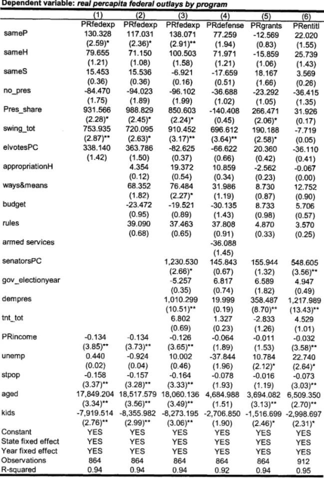
We will now ask if the results we found are robust to having a more complete specification, where different effects are considered at the same time. What we have done so far is to analyse the different hypotheses one by one, like alI the previous, and generalIy method-ologicalIy less sophisticated, empirical literature. In Table 4 we pulI together the various, and not necessarily conflicting, hypotheses.
From columns 1 and 2 it is clear that alI the results obtained on individual variables (or group of variables) are substantially confirmed by this robustness check. In the remaining regressions we aIs o add a number of further controls that previous studies have identified as determinants of federal budget alIocation. We include a variable to take into account over-representation (senators per capita, Le. senatorsPC), a dummy for having a democratic presidents (dempres) and electoral turnout in presidential elections. AIso, given the impor-tance of the relationship between president and governors, we also add a dummy equal to 1 for states and years where there is a gubernatorial election (gov_electionyear). Overrep-resentation turns out to be particularly important for direct payments to individuaIs and total spending17 while we find that gov_electionyear has a significantly positive impact on
the alIocation of grants, although rather small in magnitude (around 6.5 $ per capita). This seems to suggest that grants might have a particular importance for incumbent governors18 .
Having a democratic president substantially increases overall spending (more than 1000 $ per capita) as well as grants and direct payments to individuaIs, while it has no impact on
l70ne standard deviation of SenatorsPC is worth around 1,200 $ in per capita spending.
18It is intuitively clear that grants can give political returns to governors: thanks to the discretion they might have on how to spend grants it is well possible that voters associate that form of spending with governors much more than they do for other transfers they receive. However motivated a governor can be to obtain more grants, it remains to be asked what is the process that leads to actual allocation: in other terms we should ask who are the actors or institutions that drive such resulto We tried to include a number of interactions in order to isolate the relevant mechanism but could not render our findings any more defined.
defense spending. Finally, we do not find any evidence of an impact of turnout.
In column 3 we find again that significant explanatory variables of total federal expendi-ture per capita are the party alignment between the president and the governor, the share of presidential votes in the last election and having a high degree of swingness. The magni-tude of same_P is substantially unsensitive to the change in specification, while the relative importance of Pres_share and swing_tot is now a bit different. The difference between having maximum and minimum swing_tot amounts to 582 $ while the corresponding figure for Pres_share is 520 $. We find again confirmation of a significantly negative no_pres and the cost of opposing the president is almost 100 $ per capita. In column 3 we also find a positive effect of having members in the ways and means committee. This confirms the results that Alvarez
& Saving (1997) found in their cross-section study.
In column 4 we analyse defense spending, for which the most important explanatory variable turns out to be swing_tot. In fact, it seems that most of the effect of swing_tot
on total spending is due to defense, suggesting that defense spending could be the way swing states are targeted for election purposes. Results on the little effects of committees (including the armed service house committee) are confirmed while there is some evidence of a party alignment affect (president-governor). Some final remarks are in order. First, Democratic and Republican presidents do not seem to behave differently with respect to defense spending. Second, economic and demographic variables are definitely less impor-tant in driving defense than overall spending. One imporimpor-tant observation concerns the unemployment rate which is insignificant as an explanatory variable of federal spending, positively significant, as expected, in explaining grants and direct payments to individuaIs, but negative in the defense equation. A number of interpretations are possible, including the fact that unemployed could be less electorally responsive to pork-barrel spending. This is especially intriguing as we control for income, which shows a negative sign19 .
Column 5 reports the results for grants spending, which show good support for both the swing voter and the ideological support hypotheses. For direct payments to individuaIs instead (column 6), we find no significant effect of any of the considered variables, while it is clear that spending depends essentially on overrepresentation, having a democratic president and economic and demographic variables.
19Buying the votes of poorer citizens should be cheaper, if we believe in decreasing marginal utility of income. However, a negative coefficient of income is also compatible with purely welfaristic concerns, while this is clearly not the case for the coefficient of unemployment.
To conclude this section, our results are quite robust to change in the specification adopted and to the fact of considering various theories jointly. When we consider different spending categories, we also find some significant differences in the way different forms of public spending respond to political variables.
5. Conclusions
The alIocation of the US federal budget is a complex process that has been widely studied by political scientists. The most common idea of this process is that Congress (and particularly the House) is the place where the distribution of federal monies is decided, through a process of logrolling among non-partizan territorialIy-oriented representatives. We found that this idea is misleading.
First of alI, our study provide evidence of substantial budgetary power of the President, a player that has been neglected by most previous literature. This is clear both from the fact that presidential election results matter and from the positive effect of the president-governor party alignment. For what concerns election results, while we do not find any evidence of spending being targeted at marginal or short-term swing states, we do find support for the idea that historically volatile states tend to receive more funds. At the same time, states that show large support for the presidential party are aIs o rewarded. This two possibilities are not necessari1y incompatible, as often believed. A volatile state that always vote for the winning presidential candidate by large margins will potentially benefit the most from electoral competition: this suggest the need to look at the ideological composition of the population rather than at electoral results as way to better identify the role of the various targeting incentives.
The impact of the president-governor relationship on federal spending aIs o shows that party membership matters and that possible trades of infiuence occurs at different leveI through party lines. There are, however, a number of dimensions along which we do not find evidence of such trading occurring. OveralI, the infiuence of Congress is probably less than commonly believed. For example we do not find any strong effect of committee mem-bership, with the partial exception of the ways and mean committee. Although the budget is approved by Congress, the proposal and veto power of the President and the structure of the budgetary process (together with the very sophisticated technical support available for the drafting of the President's budget), leave a substantial space for manoeuvre to the
•
dent. Nevertheless, the role played by overrepresentation in Senate shows that the Congress has definitely an influence on spending, especially on direct payments to individuaIs.
Further research is necessary to better disentangle some of the theories we discussed. Nevertheless, by using a panel dataset with a relatively long time span, and by testing various theories on the same dataset, we have obtained comparable results on the explanatory power of alternative theories of budget allocation. More importantly, we believe to have reached new findings that are more robust and methodologically sounder when compared with previous research.
•
MMMMMMMMMMMMMMセセセセセセセセセセセセ@
References
[1] A. Alesina and G. Tabellini: "A positive theory of fiscal deficit and goverment debt" ,
Review of Economic Studies, July 1990.
[2] A. Alesina, N. Roubini and G. Cohen: Political Cycles and the Macroeconomy, Cam-bridge, Mass., MIT Press, c1997.
[3] R.M. Alvarez and J.L. Saving: "Congressional committees and the political economy of federal outalys", Public Choice 92, 55-73, 1997.
[4] C.M. Atlas, T.W. Gilligan, R.J. Hendershott and M. A. Zupan: "Slicing the Federal Government Net Spending Pie: who wins, who loses, and why". American Economic Review, vol 85, 1995.
[5] T. Besley and A. Case: "Political Institutions and Policy Choices: Evidence from the United States", Journal of Economic Literature; XLI, March 2003, pages 7-73 .
[6] T. Besley and A. Case: "Does Electoral Accountability Affect Economic Policy Choices? Evidence from Gubernatorial Term Limits", Quarterly Journal of Economics;
110(3), August 1995, pages 769-98.
[7] G.W. Cox and M.D. McCubbins: "Electoral Politics as a Redistributive Game", Jour-nal of Politics, 48, pages 370-89.
[8] M. Dahlberg and E. Johannsson: "On the Vote-Purchasing Behaviour of Incumbent Governments", American Political Science Review, 96, 27-40, 2002.
[9] A. Dixit and J. Londregan: "Redistributive Politics and Economic Efficiency" , Amer-ican Political Science Review, 89, 1995.
[10] A. Dixit and J. Londregan: "Ideology, Tactics, and Efficiency in Redistributive Poli-tics", Quarterly Journal of Economics, 113, pages 497-529, 1998.
[11] C. F. Goss: "Military Committee Membership and Defense-Related Benefits in the House of Representatives", The Western Political Quarterly, 25, 1972.
[12] S.D. Levitt and J.M. Snyder: "Political Parties and the Distribution of Federal Out-lays", American Journal of Political Science, vol 39, 958-980, 1995.
, I
[13] A. Lindbeck and J.W. Weibull: "Balanced-budget redistribution as the outcome of
political competition", Public Choice, 52, 273-97, 1987.
[14] A. Lindbeck and J.W. Weibull: "A Model of Political Equilibrium in a Representative
Democracy", Journal of Public Economics, 51, pages 195-209, 1993.
[15] G. Nelson and C.R. Bensen: Committees in the US Congress, 1947-1992, Washington,
D.C : Congressional Quarterly, 1993.
[16] D.C. North and B.R. Weingast: "Constitutions and Commitment: The Evolution of
Institutions Governing Public Choice in Seventeenth-Century England", The Journal of Economic History, 1989.
[17] J.R. Owens and L. Wade: "Federal Spending in Congressional Districts", The Western
Political Quarterly, voI. 37, 404-423, 1984.
[18] T. Persson, G. Roland and G. Tabellini: "Separation of powers and political
account-ability", Quarterly Journal of Economics;112(4), November 1997, pages 1163-1202.
[19] T. Persson and G. Tabellini: "Constitutional Rules and Fiscal Policy Outcomes" (May
2003), forthcoming in the American Economic Review.
[20] B. Ray: "Military Committee Membership in the Rouse of Representative and the
Distribution of Federal Outlays", Western Political Quarterly, 34, 1981.
[21] M. Robertson: Committees in Legislatures: a Comparative Analysis, J. D. Lees and M.
Shaw eds., Duke University Press, 1979.
[22] B. S. Rundquist and D. E. Griffith: "An Interruptuted Time-Series Test of the
Distribu-tive Theory of Military Policy-Making", The Western Political Quarterly, 29, 1976.
[23] K.A. Shepsle and B.R. Weingast (1984): "When Do Rules of Procedure Matter",
Jour-nal of Politics, 1984.
[24] G. Wright: "The Political Economy of New Deal Spending: an econometric analysis",
Review of Economics and Statistics, 56, 1974.
I ,
,
- - -
-List of variables
From the Statistical Abstract of the US and the Bureau of Statistics (alI variabIes in 2000 constant US
$)
• Fedexp: real percapita federal expenditure (outlays) by state.
• Direxp: real percapita direct payments to individuaIs (outlays) by state.
• Defense: real percapita defense expenditure (outlays) by state.
• Procurement: real percapita procurement expenditure (outlays) by state.
• Entitlements: real direct payment to individuaIs per capita.
• Grants: real grants per capita.
• PRincome: real income per capita.
• Stpop: State population.
• Turnout: total percentage of voting population in the last presidential election.
• Aged: percentage of population over 65 years old by state.
• Kids: percentage of population between 5 and 17 years old by state.
• Unemp: unemployment rate.
Authors' eIaborations on data from the StatisticaI Abstract of the United States
• SameP: dummy variable equal to one when the party affilitiation of the president and the governor is the same, and zero otherwise.
• SameH:dummy variable equal to one when the party affilitiation of the majority of the House and party affiliation of the governo r is the same, and zero otherwise.
• SameS:dummy variable equal to one when the party affilitiation of the majority of the Senate and party affiliation of the governar is the same, and zero otherwise.
20
BIBLIOTECA MARtO HF.Nf.lIQUE
S!MONSEN
-..
.,•
• Gov _electionyear: dummy variable equal to one during a governor election year and zero otherwise.
• SenatorsPC: number of senators percapita by state.
• HousePC: number of House representatives percapita by state.
• ElvotesPC: number of electoral votes percapita by states. number of senators per-capita by state.
• SameGOV _S: dummy variable equal to one when the party affilitiation of the governor and the two senators from the state are the same, and zero otherwise.
• SameGOV _H: dummy variable equal to one when the party affilitiation of the governo r and the majority in the State House are the same, and zero otherwise.
• Presclose%: distance in percentage of vote between the winner of the presidential race and the first runner up.
• Winpres: dummy variable equal to one for the state where the incumbent president has won the elections, and zero otherwise.
Authors' elaborations on information from the OffieiaI CongressionaI Direc-tory and from Nelson and Bensen (1993).
• AppropriationPC: number of appropriation committee percapita by states.
• AppmajSeniority: number of terms of the most senior House appropriation committee member and number of years of the most senior Senate appropriation committee member.
Other
• Dempres: dummy variable equal to one when the president is democratic, and zero when the president is republicano
• Termpres: dummy variable equal to one when the president faces term-limit and zero otherwise.
.
}..
•
•
•
sameH i
LLセセGB@ . . ... . . NNNセNセLNK@ ""
gov_electionyi
'sameGOV 5
iセBセG@sameGOV hiGセキキキキLセL@
Tables
セセセNLセBBGセLLセLLLLセセLLセNLキw⦅GwセB]B]KMセBB]BLLBG]G@
22
Max
9180.842
4r- • l J
..
..
•
•
•
•
labia 1 : Committee Influence
Dependent variable: real percapita outlays by program
!1 セ@ ARセ@ ASセ@ ATセ@ AUセ@ AVセ@
PRfedexp PRfedexp PRdefense PRdefense PRgrants PRentitl appropriations -35.2783 6.5788 -15.7951 -15.4699 (0.95) (0.21) (1.19) (1.09) ways&means 13.2584 32.6421 -7.2686 -5.8983
(0.27) (1.36) (0.59) (0.37)
budget -28.0054 -32.7585 7.3641 4.3059
(1.08) (1.46) (0.76) (0.43)
rules 6.1463 36.9675 -6.5793 -8.5665
(0.11 ) (0.90) (0.36) (0.57)
armed serv -30.8435 -33.7949
(1.21 ) (1.33)
PRincome -0.1091 -0.1019 -0.0627 -0.0623 -0.0030 -0.0314 (6.40)** (3.11 )** (1.92) (1.86) (0.37) (2.65)* unemp -1.8968 -10.1416 -38.3475 -40.2883 6.9869 16.2695
(0.19) (0.44) (2.09)* (2.15)* (1.18) (1.74) stpop -0.1338 -0.1186 -0.0700 -0.0718 -0.0053 -0.0577
(6.40)** (2.57)* (1.67) (1.80) (0.38) (2.53)* aged 16,251.6839 17,382.4885 4,110.0100 4,548.1978 3,581.4413 6,814.5308
(4.65)** (3.16)** (1.32) (1.48) (2.87)** (2.73)** kids -6,690.4641 -7,240.7223 -2,342.7220 -2,611.3896 -1,288.9445 -2,902.9315
(3.54)** (2.38)* (1.67) (1.86) (1.97) (2.08)*
Constant YES YES YES YES YES YES
State fixed effects YES YES YES YES YES YES Year fixed effects YES YES YES YES YES YES
Observations 912 864 864 864 864 912
R-squared 0.92 0.93 0.92 0.92 0.93 0.94
OLS regressions; Robusl I slalislics in parenlheses (' significanl aI 5%;" significanl aI 1%)
MMMMMセ@ _ .. - - MMセMMMMM
-labia 2: Swing and Ideological Bias
Dependent variable: real percapita federal outlays
サQセ@ セRセ@ セSセ@ セTセ@ セUセ@
PRfedexp PRfedexp PRfedexp PRfedexp PRfedexp
Pres_shareW60 1,704.7198 1,821.4292 1,298.7982 1,710.3441
(2.24)* (2.75)** (2.61 )* (2.25)*
prescloseW60 -382.1046 -615.1480 -381.5436
(0.69) (1.46) (0.69)
elvotesW60 -4.3200
(0.16)
elvotesPCW60 386.0369
(1.72) swing_stateW60
swing_tot 533.4176 558.8974 118.2320
(1.82) (1.89) (0.33)
win_stateW60 -75.4743
(0.67)
INT _swing_winW60 378.8953
(1.35)
PRincome -0.1262 -0.1278 -0.1254 -0.1256 -0.0991
(3.76)** (3.71 )** (3.88)** (3.85)** (3.13)**
unemp -7.3322 -0.2502 -8.3565 -7.5952 -7.4981
(0.35) (0.01 ) (0.40) (0.35) (0.33)
stpop -0.1318 -0.1540 -0.1309 -0.1365 -0.1312
(2.51 )* (3.14)** (2.57)* (2.68)* (2.88)**
aged 18,229.9432 17,735.8026 18,218.8693 18,242.5852 16,357.7928
(3.37)** (3.39)** (3.36)** (3.37)** (2.96)**
kids -7,982.3003 -7,871.8075 -7,938.9665 -7,990.4876 -6,787.4619
(2.74)** (2.81 )** (2.72)** (2.75)** (2.23)*
Constant YES YES YES YES YES
State fixed effect YES YES YES YES YES
Year fixed effect YES YES YES YES YES
Observations 864 864 864 864 864
R-squared 0.93 0.94 0.93 0.93 0.93
OLS regressions; Robusl I slalislics in parenlheses ( • significanl ai 5%; •• significanl ai 1 %)
•
•
'W" f { À
.,
•
•
•
•
Table 3: Party Allignment
Dependent variable: real percapita federaloutlays
samePW60 sameHW60 sameSW60 senate_majW60 nOJ)resW60 PRincome unemp stpop aged kids Constant State fixed effect Year fixed effect Observations R-squared
(1) (2) (3)
PRfedexp PRfedexp PRfedexp 134.9037 (2.35)* 100.7199 (1.54) 12.3287 (0.28) -39.4412 (0.99) -74.9903 (1.39) 60.4875 (0.91) (4) PRfedexp -154.6240 (2.61)* -5.9300 (0.14) (5) PRfedexp 136.5705 (2.39)* 99.3193 (1.45) 30.7023 (0.70) -0.3764 (0.01) -106.3987 (1.68) 29.4614 (0.52) -142.7461 (2.32)* 38.3668 (0.79) (6) PRfedexp 137.9171 (2.52)* 100.0778 (1.56) 36.8956 (0.86) -5.3423 (0.11 ) -99.7257 (1.60) 22.1627 (0.39) 71.0014 (0.93) 36.5556 (0.76) -235.2727 (3.02)** -0.1001 -0.1059 -0.1009 -0.1145 -0.1212 -0.1241 (3.02)** (3.29)** (3.10)** (3.59)** (3.73)** (3.86)** -7.1561 -5.5811 -7.4937 -7.4440 -2.1096 0.8093 (0.32) (0.24) (0.33) (0.33) (0.10) (0.04) -0.1301 -0.1265 -0.1331 -0.1507 -0.1476 -0.1540 (3.01 )** (2.74 )** (2.71 )** (3.09)** (3.15)** (3.27)** 17,144.5028 17,680.1559 16,757.8809 17,458.6030 17,299.3163 17,346.7710
(3.31)** (3.29)** (3.24)** (3.02)** (3.05)** (3.08)** -7,079.9063 -7,570.4469 -7,060.3568 -7,584.5133 -7,675.9732 -7,670.8147
(2.49)* (2.54)* (2.51)* (2.42)* (2.51)* (2.52)*
YES YES YES YES YES YES
YES YES YES YES YES YES
YES YES YES YES YES YES
864 864 864 864 864 864
セイッ@ セイッ@ セイッ@ セイッ@ セイッ@ セイッ@
OLS regressions; Robusl I slalislics in parenlheses (' significanl aI 5%;" significanl aI 1%)
'li
Table 4: Ali theories
Dependent variable: real percapita federal outlays by program
(1 ) (2) (3) (4) (5) (6)
4 PRfedexp PRfedexp PRfedexp PRdefense PRgrants PRentitl
sameP 130.328 117.031 138.071 77.259 -12.569 22.020 (2.59)* (2.36)* (2.91 )** (1.94) (0.83) (1.55)
..
sameH 79.655 71.150 100.503 71.971 -15.859 25.739 (1.21 ) (1.08) (1.58) (1.21 ) (1.06) (1.43) sameS 15.453 15.536 -6.921 -17.659 18.167 3.569 (0.36) (0.36) (0.16) (0.51 ) (1.66) (0.26) no_pres -84.470 -94.023 -96.102 -36.688 -23.292 -36.415(1.75) (1.89) (1.99) (1.02) (1.05) (1.35) Pres_share 931.566 988.829 850.603 -140.408 266.471 31.926 (2.28)* (2.45)* (2.24)* (0.45) (2.06)* (0.17) swing_tot 753.935 720.095 910.452 696.612 190.188 -7.719 (2.87)** (2.63)* (3.17)** (3.64)** (2.58)* (0.05) elvotesPC 338.140 363.786 -82.625 -66.622 20.360 -36.110
(1.42) (1.50) (0.37) (0.66) (0.42) (0.41 ) appropriationH 4.354 19.372 10.859 -2.562 -0.067 (0.12) (0.54) (0.34) (0.23) (0.00) ways&means 68.352 76.484 31.986 8.730 12.752
(1.82) (2.27)* (1.19) (0.87) (0.90) budget -23.472 -19.521 -30.135 8.733 5.706 (0.95) (0.89) (1.43) (0.98) (0.57)
rules 39.090 37.463 37.808 4.870 3.570
(0.68) (0.65) (0.91 ) (0.33) (0.25)
armed services -36.088
(1.45)
senatorsPC 1,230.530 145.843 155.944 548.605 (2.66)* (0.67) (1.32) (3.56)** gov _ electionyear -5.257 6.817 6.589 4.947
(0.35) (0.74) (1.82) (0.49) dempres 1,010.299 19.999 358.487 1,217.989
(10.51 )** (0.19) (8.70)** (13.43)**
tnUot 6.802 1.327 -2.833 4.529
(0.69) (0.23) (1.26) (1.01) PRincome -0.134 -0.134 -0.126 -0.064 -0.011 -0.032 (3.85)** (3.73)** (3.65)*- (1.89) (1.53) (3.58)*-unemp 0.440 -0.924 10.002 -37.844 10.784 22.740 (0.02) (0.04) (0.46) (1.96) (2.12)* (2.64)-stpop -0.158 -0.157 -0.164 -0.078 -0.016 -0.073 (3.37)-' (3.28)*' (3.33)*- (1.93) (1.19) (3.03)-* aged 17,849.204 18,517.579 18,060.136 4,684.988 3,694.082 6,509.350
(3.34)-- (3.56)'- (3.49)'- (1.51) (3.13)-- (2.70)*-kids -7,919.514 -8,355.982 -8,273.195 -2,706.850 -1,516.699 -2,998.697
(2.76)-- (2.99)** (3.06)** (1.90) (2.46)' (2.31 )*
Constant YES YES YES YES YES YES
State fixed effect YES YES YES YES YES YES Year fixed effect YES YES YES YES YES YES
Observations 864 864 864 864 864 912
R-squared 0.94 0.94
..
0.94 0.92 0.94 0.95OLS regressions; Robusl I stalislics in parenlheses ( • significanl ai 5%; *. significanl ai 1 %)
..
...
..
26
9j'2Y1
_ ... " = . -BIBliOTECA MY:-."] hZ]セAイZZ]iue@ SiMONSEN
; ;;iú,;ÇI\U GtJÚUO vaNr⦅セセセ@ ..
000349481