UNIVERSIDADEFEDERAL DEMINASGERAIS INSTITUTO DECIÊNCIASEXATAS DEPARTAMENTO DEESTATÍSTICA
PROGRAMA DEPÓS-GRADUAÇÃO EMESTATÍSTICA
Sistemas Prospectivos para
Vigilância Espaço-tempo
Thais Rotsen Correa
Tese de doutorado submetida à Banca Examinadora desig-nada pelo Colegiado do Programa de Pós-Graduação em Es-tatística da Universidade Federal de Minas Gerais, como re-quisito parcial para obtenção do título de Doutor em Estatís-tica.
Orientador: Prof. Dr. Renato Martins Assunção
Agradecimentos
Este trabalho não teria sido possível sem a ajuda de muitas pessoas, às quais agradeço imensamente.
Agradeço em primeiro lugar a Deus, por me iluminar, me dar força e saúde durante toda esta caminhada.
À minha família que eu amo tanto, e que é a minha base. Ao meu pai, que sempre vibrou com as minhas vitórias. À minha mãe, que esteve sempre ao meu lado me motivando e me ajudando. À minha irmã, pela amizade e confiança.
Ao Felipe, por todo amor, carinho e paciência, por me fazer feliz! À Fátima e Bia, que sempre me apoiaram.
Aos amigos da UFOP, que sempre acreditaram no meu sucesso. Em especial, agradeço ao Anderson pelas várias ajudas, sem as quais teria sido tudo muito mais difícil. Ao Júlio e ao Flávio, pelos cafés providencias para esfriar a cabeça.
Ao Renato, por todos estes anos de orientação e ensinamentos e pelo exemplo de profis-sional que é e sempre foi para mim.
Ao pessoal do LESTE, sempre presente em partes importantes (e divertidas) desta cami-nhada.
Aos professores e funcionários do Departamento de Estatística da UFMG, em especial ao Marcelo e à Rogéria.
Aos membros da banca, professores Glaura Franco, Fábio Demarqui, Francisco Louzada Neto e Ronaldo Dias, pelas sugestões e considerações.
Resumo
A demanda por sistemas capazes de detectar mudanças nos padrões espacial e tempo-ral de ocorrência de eventos tem crescido em diversas áreas do conhecimento. Os avanços tecnológicos ocorridos nos últimos anos facilitaram a coleta e análise da informação geo-gráfica, causando um aumento no interesse por sistemas para detecção de conglomerados espaço-tempo. O estudo deste tipo de sistema é recente e ainda existem poucas propostas.
Abstract
The demand for systems capable of detecting changes in spatial and temporal patterns of occurrence of events has grown in several areas of the knowledge. Technological advances in recent years have facilitated the collection and analysis of geographic information, causing an increase in interest in systems for detecting space-time clusters. The study of this type of system is still new and there are few proposals.
Sumário
1 Introdução 12
1.1 Métodos de Vigilância em Controle de Qualidade . . . 14
1.2 Métodos Espaço-temporais Prospectivos . . . 16
2 Objetivos 18 2.1 Objetivos Gerais . . . 18
2.2 Objetivos Específicos . . . 18
3 Organização 19 4 Tempo Médio de Espera pelo Alarme 20 5 Sistema de Vigilância Shiryayev-Roberts 22 5.1 Descrição do Sistema SR . . . . 22
5.2 Vantagens do Sistema SR . . . . 23
6 Vigilância espaço-tempo para detecção de conglomerado emergentes 25 6.1 Abstract . . . 25
6.2 Introduction . . . 25
6.3 Prospective space-time surveillance for localized clusters . . . 27
6.4 Detection of emerging space-time clusters . . . 30
6.4.1 A model for emerging clusters . . . 30
6.4.2 A sequential procedure to detect emerging clusters . . . 32
6.4.3 Estimation of µ(Ck,n) . . . 33
6.4.4 Iterative calculation of Rn . . . 35
6.5 Choice of tuning parameters . . . 36
6.6 Method performance . . . 38
6.6.1 Scenario without clusters . . . 39
6.6.2 Scenarios with clusters . . . 40
6.7 Illustrative examples . . . 42
6.7.1 Burkitt’s lymphoma cases in Uganda . . . 42
6.7.2 Meningitis cases in Belo Horizonte . . . 47
7 Vigilância espaço-tempo prospectiva para dados de área 51
7.1 Abstract . . . 51
7.2 Introduction . . . 51
7.3 Statistical formulation . . . 53
7.3.1 Monitoring statistic . . . 53
7.3.2 Expected value for the monitoring statistic . . . 56
7.3.3 Specification of the threshold A . . . . 57
7.3.4 Estimation of µCk,n . . . 58
7.4 Simulation study . . . 59
7.4.1 Simulation results for an under control process . . . 59
7.4.2 bµCj,k versus µCj,kfor under and out of control processes . . . 60
7.4.3 Impact of the spatial size of the cluster . . . 63
7.5 Illustrative example . . . 63
7.6 Final considerations . . . 65
8 Um olhar cuidadoso sobre vigilância prospectiva usando uma estatística scan 66 8.1 Abstract . . . 66
8.2 Introduction . . . 66
8.3 The Scan Statistic for Emerging Outbreaks . . . 69
8.3.1 Kulldorff (2001) . . . 69
8.3.2 Tango et al. (2011) . . . 70
8.4 Simulation Results . . . 72
8.5 Final Considerations . . . 79
9 Sistemas Alternativos 81 9.1 Passeio aleatório com barreiras . . . 81
9.1.1 Passeio aleatório com uma barreira absorvente em 0 e uma barreira refletora em b>0 . . . 81
9.1.2 Passeio aleatório com uma barreira absorvente em b>0 e uma bar-reira refletora em 0 . . . 82
9.1.3 Passeio aleatório no contexto de vigilância . . . 82
9.2 Sistemas de vigilância para dados pontuais . . . 83
9.2.1 Sistema Binário . . . 84
9.2.2 Sistema Padronizado . . . 84
9.2.4 Determinação da constante c . . . . 85
9.2.5 Esperança e Variância de Zne Zn∗. . . 88
9.3 Estudo de simulação . . . 89
9.3.1 Resultados preliminares . . . 90
9.3.2 Modelo exponencial . . . 91
9.4 Considerações finais . . . 105
10 Considerações Finais 106
Apêndice 107
Lista de Figuras
1 Exemplo de um processo pontual espaço-temporal a tempo contínuo visua-lizado como um conjunto de setas no espaço tridimensional, onde cada seta representa um evento. A altura da seta é igual à coordenada temporal. . . 13 2 The estimate ˆµ(Ck,n) . . . 34
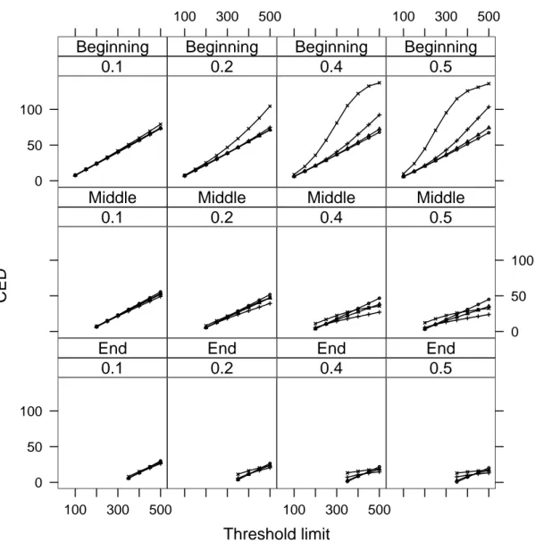
3 Scenario without cluster. The plots show the estimated ARL0=E(TA), the average number of events observed before a false signal is issued, versus the threshold limit A. Each curve corresponds to a value of ε. In all cases, we usedρ=1. . . 40 4 Estimated CED∗(τ) against the values of the threshold A. The first row of
plots corresponds to the homogeneous scenarios (Hom) while the second row corresponds to the inhomogeneous scenarios (Inh). The different columns correspond to different values of ε. Each plot has three lines. The circles correspond to case B, when the cluster emerges soon in the observation period (τ=50). The crosses correspond to case M (τ= 150), and the triangles correspond to case L (τ=300). . . 43 5 Left hand side: False alarm rates versus threshold limit A for the scenarios
when the cluster emerges on the middle of the observation period with ε= 2.5,5,10,20. Right hand side: Idem for cluster emerging at the end of the observation period. . . 44 6 Effect of changingρ. The rows correspond to the three cluster emerging time
τ=50,150,300, and the columns correspond to different values of ε. Only the homogeneous case was considered. The curves with circles correspond toρ=0.25, the curves with triangle toρ=0.5, the curves with crosses to
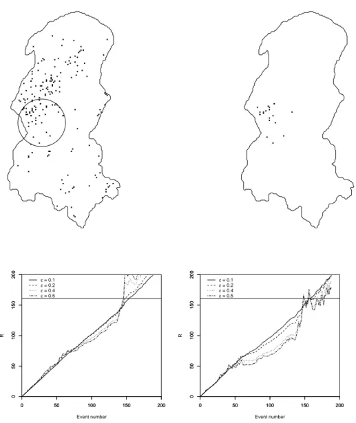
ρ=1.0, and the curves with axes toρ=2.0. The true value ofρis 0.5. . . . 45 7 Burkitt’s lymphoma cases in West Nile district of Uganda from 1961 to 1975
(study region is approximately 80 km× 170 km). The left hand side map shows all the events in the period while the right hand side map shows the events identified in the emerging cluster by our method. Each one of the plots shows Rn versus n for four different choices ofε: 0.1,0.2,0.4, and 0.5. The left hand side plot uses ρ=10 km and the right hand side plot uses
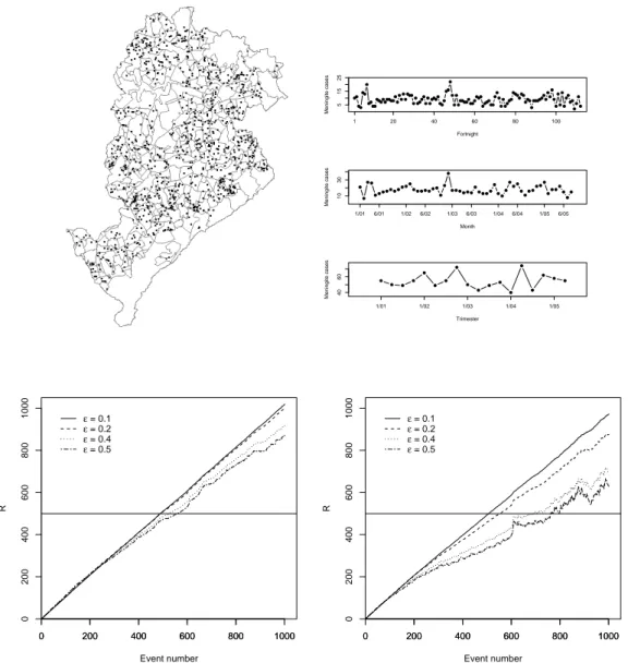
8 Map of Belo Horizonte divided into neighborhoods and the location of 1001 Meningitis cases that occurred between 2001 and 2005. The study region has approximately 31 km × 16 km. The time series plots show the number of events in different time units: fortnightly, monthly, and quarterly. Each one of the plots shows Rn versus n for four different choices of ε: 0.1,0.2,0.4, and 0.5. The threshold is A=500. The left hand side plot usesρ=1 km and the right hand side plot usesρ=2 km. . . 49 9 Time m (horizontal axis) versus the trimmed average value of Rm, taken over
300 simulations, divided by µ (vertical axis). The trimmed average value excludes the highest and lowest 1% of the data points. Rows 1,2,3,4 cor-respond toρ=0.0,1.0,1.5,2.0, respectively. Columns 1,2,3 correspond to
ε=0.01,0.03,0.05, respectively. The dashed and dotted lines correspond to Rm calculated with µCj,k andbµCj,k, respectively. The solid line represents
Eτ=∞(Rm)divided by µ. . . . 61
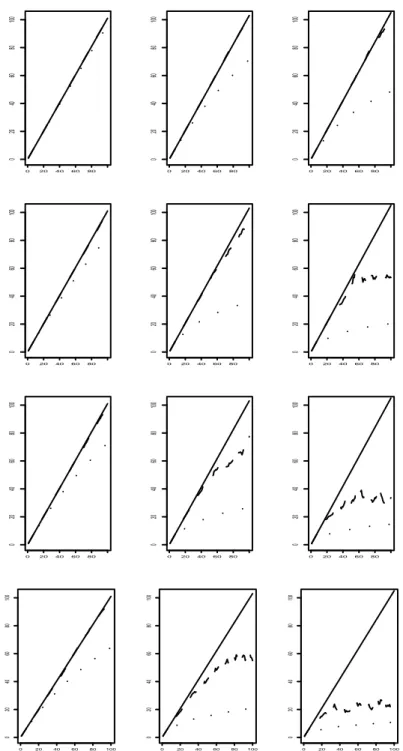
10 Summary statistics for the number of time periods until the alarm sounds off in 300 simulations, using an under control process. Rows 1,2,3,4 correspond to ρ=0.0,1.0,1.5,2.0, respectively. Columns 1,2,3,4 corresponds to ε= 0.20,0.25,0.30, respectively. The horizontal axis represents the threshold limit: 20,30,40 time periods. The vertical axis represents the number of time periods until the alarm sounds off. The circles and the triangles represents the average value using µCj,k andbµCj,k, respectively. The segments in each
symbol represents one standard deviation above and below the mean. The numbers at the bottom and at the top correspond to the proportion of alarms when using µCj,k andbµCj,k, respectively. . . 94
11 Summary statistics for the number of time periods until a motivated alarm in 300 simulations, using an out of control process. Rows 1,2,3,4 correspond to ρ=0.0,1.0,1.5,2.0, respectively. Columns 1,2,3,4 corresponds to ε= 0.20,0.25,0.30, respectively. The horizontal axis represents the threshold limit: 20,30,40 time periods. The vertical axis represents the number of time periods until the alarm sounds off. The circles and the triangles represents the average value using µCj,kandbµCj,k, respectively. The segments in each symbol
12 Summary statistics for the observed number of time periods until a motivated alarm in 300 simulations, considering an out of control process. Each plot corresponds to one value forρ. In all plots, the horizontal axis represents the threshold limit: 20,30,40 time periods. The vertical axis represents the ob-served number of time periods until the motivated alarm. The traces, crosses, and lozenges represent the average value for ε=0.20,0.25,0.30, respecti-vely. The segments in each symbol represents one standard deviation above and below the mean. The numbers at the top corresponds to the proportion of motivated alarms. For each threshold limit, the first, second and third num-bers are related toε=0.20,0.25,0.30, respectively. . . 96 13 Meningococcal cases in Germany between 2002 and 2008. The federated
sta-tes are: 1=Baden-Württemberg, 2=Bayern, 3=Berlin, 4=Brandenburg, 5=Bre-men, 6=Hamburg, 7=Hessen, 8=Mecklenburg-Vorpommern, 9=Niedersach-sen, 10=Nordrhein-Westfalen, 11=Rheinland-Pfalz, 12=Saarland, 13=Sach-sen, 14=Sachsen-Anhalt, 15=Schleswig-Holstein, 16=Thüringen. . . 97 14 Number of cases per year/quarter. . . 98 15 Monitoring statistic R at each quarter. The solid, dashed and dotted lines
corresponds toε=0.20,0.25,0.30, respectively. . . 98 16 Results for the retrospective scan - situation (a). The first graph shows in solid
line the average critical value for the scan statistic together with the pointwise 95% confidence bands L(n) and U(n) in dashed lines. The second graph shows in solid line the average p-value together with the 95% confidence bands for the observed p-value at each time series length n (in dashed lines). The third graph shows the proportion of simulations in which the p-value is at mostα. . . 99 17 Results for situation (b) when the prospective scan has no adjustment for
earlier analysis. In all the three graphs, the lines (solid and dashed) have the same definition as in Figure 16. . . 99 18 Results for situation (c) when the prospective scan adjusts for all previous
analysis. Definitions of lines and plots are the same as in Figure 16. . . 100 19 Results for situation (c) when the prospective scan adjusts for the last 100
20 In each row, the first plot illustrates the typical behavior of the p-value time series pt. The second and the third plots show the distribution of the range and the variance for all 1000 time series pt, respectively. . . 101 21 SaTScan p-value versus the p*-value for the prospective scan adjusting for
all previous analysis. . . 101 22 RL∗versus RI∗for the prospective situations (c) and (d). The axes are in the
logarithm scale. The proportion of alarms is 0.38 and 1.00 for situations (c) and (d), respectively. . . 102 23 Tempo médio até o alarme versus limite A. . . 102 24 Distribuição do número de eventos até o alarme no método SSR, dado que
o processo está sob controle. No gráfico da esquerdaε=0,5; no gráfico da direitaε=2,0. O limite A=ARL=650 eventos. . . 103 25 Distribuição do número de eventos até o alarme nos métodos alternativos,
dado que o processo está sob controle. Da esquerda para a direita: método Binário, método Padronizado e método Padronizado com Constante. O limite
Lista de Tabelas
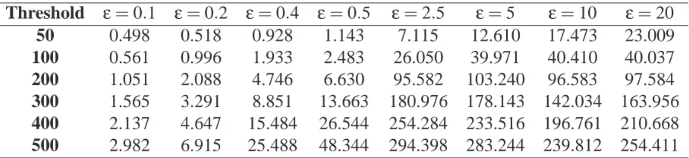
1 Standard deviation of the stopping time TA for different choices of threshold
A andε. In all cases we usedρ=1. . . 40 2 In each cell, the first value is the number of quarters until the alarm sounds
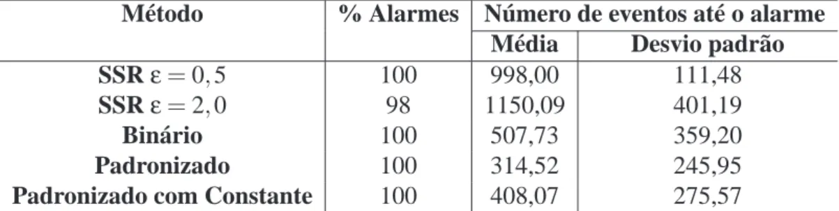
off, and the second one is the estimate for the spatial location of the cluster (identification number of the state). NA means that the alarm did not sound off. 65 3 Estatísticas referentes a 100 simulações de um processo sob controle, onde
δ=3 nos sistemas alternativos e ARL=650 eventos. No método SSR, o limite A=ARL. Nos métodos alternativos, A=√ARL. A coluna % Alarmes
mostra o proporção de alarmes. . . 91 4 Proporção de alarmes falsos e motivados em 100 simulações utilizando-se
processos fora de controle, ondeδ=3 nos métodos alternativos e ARL=650 eventos. No método SSR, o limite A=ARL. Nos métodos alternativos, A=
√
ARL. . . . 92 5 Estatísticas baseadas em 50 simulações dos métodos alternativos e 100
si-mulações do método SSR para processos fora de controle, onde ε=0,5 no método SSR,δ=3 nos métodos alternativos, ARL=650 e λ1=6. No mé-todo SSR, o limite A=ARL=650 eventos. Nos métodos alternativos, A=69 eventos. . . 104 6 Estatísticas baseadas 50 simulações dos métodos alternativos e 100
simula-ções do método SSR para processos fora de controle, ondeε=2,0 no método
SSR,δ=3 nos métodos alternativos, ARL=650 eλ1=12 No método SSR, o limite A=ARL=650 eventos. Nos métodos alternativos, A=69 eventos. . 104 7 Estatística baseadas em 1000 simulações de processos fora de controle, onde
δ=3 eλ1=6. O limite A=69 eventos. . . 105 8 Estatística baseadas em 1000 simulações de processos fora de controle, onde
1
Introdução
Atualmente, os registros feitos pela maioria das agências de saúde pública trazem infor-mações sobre o tempo e o local de ocorrência dos casos das principais doenças que atingem uma população. A informação geográfica é coletada e analisada regularmente, através do uso de softwares de geoprocessamento.
Uma vez que os registros são atualizados com uma frequência cada vez maior, as agências passaram a demandar métodos e softwares apropriados para a detecção precoce de mudanças nos padrões espacial e temporal de ocorrência destes eventos. Este tipo de método é útil não apenas no contexto de saúde pública. Métodos para detecção prospectiva de mudanças no padrão espacial ou temporal dos valores de um processo estocástico, de forma rápida e eficiente, são de grande interesse em diversas áreas do conhecimento, tais como vigilância de acidentes de trânsito, crimes em grandes cidades, dinâmica ecológica, etc.
Nesta tese, são estudados métodos prospectivos de vigilância espaço-temporal. Dois tipos de dados estatísticos são considerados. O primeiro deles é constituído pelos processos pontu-ais espaço-temporpontu-ais. Neste tipo de dados, observamos eventos pontupontu-ais da forma(xi,yi,ti), onde(xi,yi)são as coordenadas geográficas e tié a coordenada temporal do evento. Exem-plos de situações dando origem a este tipo de dados são as ocorrências de uma doença dentro de uma região geográfica e o monitoramento de queimadas na Amazônia.
O segundo tipo de dados considerado são os dados de área. Considere uma região geográ-fica particionada em H áreas denotadas por i=1, . . . ,H. A observação na área i no instante de
tempo t será denotada por yit. Neste trabalho, os dados de área terão sempre uma estrutura de tempo discreto com t=1,2, . . .Assim, os dados podem ser vistos como uma série temporal de mapas onde, em cada tempo t, temos um mapa composto pelas observações y1t, . . . ,yHt.
Com estes dois tipos de dados, estaremos ocupados em estudar métodos de vigilância prospectiva. Para isto, é útil ver as duas estruturas de dados como processos estocásticos
{X(t); t>0}, onde X(t)depende do tipo de dado. No caso de dados de processos pontuais a tempo contínuo, temos
X(t) ={N(x,y,t)},
onde N(x,y,t)é o número de eventos ocorridos na posição(x,y)desde o início do processo em t=0 até um instante arbitrário t. Seja Yit a variável aleatória observada na área i no tempo
t. No caso de dados de área, temos
o mapa de valores de Yit no instante t.
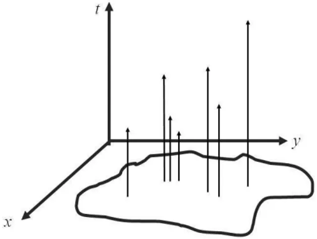
No caso de processos pontuais ditos simples, temosP(N(x,y,t)≥2) =0 para todo(x,y,t). Isto é, em cada posição(x,y), podemos ter no máximo um evento em qualquer instante de tempo. Isto significa que o processo pontual espaço-temporal a tempo contínuo pode ser equivalentemente visualizado como um conjunto de pontos ou de setas no espaço tridimensi-onal. A Figura 1 mostra um exemplo de eventos de um processo pontual vistos desta forma. Cada evento é representado por uma seta. A coordenada temporal t é dada pela altura da seta.
Figura 1: Exemplo de um processo pontual espaço-temporal a tempo contínuo visualizado como um
conjunto de setas no espaço tridimensional, onde cada seta representa um evento. A altura da seta é igual à coordenada temporal.
Assuma que existe um modelo descrevendo a distribuição do processo estocástico X(t). Isto é, existe uma família consistente de distribuições{
F
t,t >0}tal queF
t descreve a dis-tribuição da família {X(s),0≤s≤t}. Seja τ o instante em que ocorre uma mudança no processo X(t). O instanteτé desconhecido. Se a distribuição do processo não mudar, entãoτ=∞. Dizemos que o processo está sob controle em um tempo qualquer t seτ>t. Quando t>τ, dizemos que o processo está fora de controle em t.
Um sistema de vigilância prospectivo pode ser definido como um critério para decidir, em cada instante de tempo t, se o processo está sob controle ou não. Quando temos evidência suficiente de que o status do processo mudou do estado sob controle para o estado fora de controle, dizemos que temos um alarme. Podemos ter um alarme no instante t<τ. Neste caso, temos um falso alarme. Alternativamente, podemos ter um alarme soando num instante
t>τ. Neste caso, temos um alarme motivado.
É claro que esta situação ideal dificilmente ocorre na prática. Assim, almejamos encontrar um sistema em que o alarme soe pouco quando o processo está sob controle, e que seja rá-pido para detectar mudanças no processo, quando elas acontecerem. A área do conhecimento denominada estatística já desenvolveu vários métodos de vigilância no caso puramente tem-poral. Esta área da estatística é conhecida como Controle de Qualidade (veja Ryan, 1989, Wetherill and Brown, 1991 e Montgomery, 1996).
1.1
Métodos de Vigilância em Controle de Qualidade
Suponha que o processo estocástico é simplesmente uma série temporal Y1,Y2, . . .. A dis-tribuição
F
t corresponde à distribuição do vetor t-dimensional(Y1, . . . ,Yt). QuandoF
t muda de um modelo para outro, o status do processo muda de sob controle para fora de controle. No caso mais simples possível, suponha que Y1,Y2, . . .sejam independentes e identicamente dis-tribuídas com distribuição acumulada F0(y). No instanteτ, as variáveis aleatórias Yipassam a seguir a distribuição acumulada F1(y). O interesse é soar um alarme o mais rapidamente possível apósτe, ao mesmo tempo, evitar que o alarme soe enquanto t<τ.Um dos métodos mais utilizados é a carta de controle de Shewart (veja, por exemplo, Ryan, 1989, Wetherill and Brown, 1991 e Montgomery, 1996). Este método assume que
Y1,Y2, . . .são variáveis aleatórias independentes e identicamente distribuídas tal que F0(y)é a distribuição acumulada Normal com média µ e variânciaσ2. A carta de contole de Shewart soa um alarme no tempo t se o valor de Yt for inferior a um limite Liou superior a um limite
Ls. Os limites Lie Lsda carta de Shewart são dados por
Li=µ−cσ e Li=µ+cσ,
onde c é a distância dos limites de controle Lie Ls em relação à µ, expressa em unidades de desvio padrão.
Em geral, usa-se c=3. Se Yt∼Normal(µ,σ2), entãoP(µ−3σ≤Yt≤µ+3σ) =0,9973. Logo, se yt ∈/[µ−3σ,µ+3σ], temos um forte índicio de que a distribuição subjacente de Yt não é mais Normal(µ,σ2).
1991 e Montgomery, 1996). A soma acumulada no tempo t é dada por
St=max(0,St−1+yt−k),t≥1,S0=0,
onde k é uma constante que depende apenas dos parâmeros das distribuições acumuladas
F0(y)e F1(y).
O método de somas acumuladas (CUSUM) soa um alarme no tempo t se St excede um limiar h. A escolha do limiar h está associada ao Average Run Length (ARL), definido como o tempo médio até que o alarme soe dado que o processo está sob controle. O ARL será definido formalmente na seção 4. Valores altos de h estão associados a valores altos para o ARL e valores baixos de h estão associados a valores baixos para o ARL. Nos casos em que o valor do ARL é alto, teremos poucos alarmes falsos, mas mudanças reais no status do processo não serão detectadas tão rapidamente. Da mesma forma, quando o valor do ARL é baixo, as mudanças reais geralmente serão detectadas mais rapidamente, mas alarmes falsos também serão mais freqüentes.
A constante k é escolhida de forma que, para um dado limiar h, k minimiza o tempo médio necessário para que o alarme soe motivadamente. Se F0(y)é a distribuição acumulada Poisson com médiaλ0e F1(y)é a distribuição acumulada Poisson com médiaλ1, então
k= λ1+λ0 log(λ1) +log(λ0)
.
Se F0(y) é a distribuição acumulada Normal com média µ0 e variância σ2 e F1(y) é a distribuição acumulada Normal com média µ1 e variância σ2, então k = (µ0+µ1)/2. Se
µ1=µ0+2wσ, então St acumulada acumula desvios da média µ0 que excedem w desvios padrão
St=max(0,St−1+yt−µ0−wσ),t≥1,S0=0.
ponto de mudança k. Quando esta estatística ultrapassa um certo limiar, o alarme soa. O sistema proposto por Kenett and Pollak (1996) é descrito na seção 5.
1.2
Métodos Espaço-temporais Prospectivos
Existe hoje um grande interesse em estender sistemas de vigilância puramente temporais para o caso espaço-tempo, devido à demanda originada pela recente facilidade na coleta da informação geográfica. No contexto de vigilância espaço-tempo, os métodos são recentes e ainda não há nenhum método amplamente aceito como sendo superior aos demais. Descre-vemos a seguir algumas das recentes propostas de métodos espaço-temporais para vigilância prospectiva.
Kulldorff (2001) sugere o uso da estatística scan espaço-tempo, baseada na estatística scan espacial (Kulldorff, 1997), para monitoramento prospectivo de doenças em dados de área. A varredura no caso espaço-tempo é feita sob todos os cilindros vivos e busca-se aquele que maximiza a razão de verrossimilhança, baseada no modelo Poisson ou Bernoulli.
Rogerson (2001) propôs o uso de uma estatística de Knox local para monitoramento de conglomerados espaço-temporais. Marshall et al. (2007) demonstrou que, para um processo sob controle, o tempo de espera até o alarme do método proposto por Rogerson (2001) é influenciado pela densidade populacional e pela forma da região. Como consequência, o valor nominal das medidas de desempenho não são válidas. Marshall et al. (2007) também encontrou vários problemas com as aproximações usadas em Rogerson (2001).
Kulldorff et al. (2005) desenvolveram uma estatística scan espaço-tempo de permutação que não requer dados da população de risco. Uma das vantagens desta estatística é que ela pode ser aplicada a dados de processos pontuais.
Diggle et al. (2005) e Rodeiro and Lawson (2006) sugeriram métodos bayesianos para modelar a evolução espaço-temporal de taxas de incidência e monitorar mudanças.
Takahashi et al. (2008) propuseram uma estatística scan espaço-tempo flexível para de-tecção de conglomerados não circulares. Ao contrário da estatística scan espaço-tempo de Kulldorff (2001), que considera uma janela cilíndrica tridimensinal de base circular, a es-tatística scan flexível considera uma janela prismática tridimensinal cuja base tem formato arbitrário.
esperado não condicional.
Corberán-Vallet and Lawson (2011) aplicam a ordenada preditiva condicional ao contexto de vigilância para detectar pequenas áreas em que a incidência de uma doença é maior. A ordenada preditiva condicional é uma ferramenta bayesiana que permite detectar observações atípicas.
Frisén et al. (2011) consideram o caso de vigilância multivariada. Eles estudam processos em que as mudanças ocorrem simultaneamente ou em intervalos de tempo conhecidos. O princípio da suficiência é utilizado para esclarecer a estrutura de alguns problemas, encontrar métodos eficientes e determinar métricas de avaliação apropriadas.
2
Objetivos
2.1
Objetivos Gerais
Os dois principais objetivos desta tese são:
1. Desenvolver sistemas de vigilância espaço-tempo prospectivos para detecção de con-glomerados emergentes.
2. Analisar alguns aspectos dos sistemas de vigilância baseados na estatística scan pro-posta por Kulldorff (2001).
2.2
Objetivos Específicos
O primeiro objetivo desta tese é desenvolver sistemas de vigilância para dados pontuais e dados de área. Buscamos métodos automáticos, com pouca interferência do usuário e que não exijam a especificação dos padrões marginais espacial e temporal. A taxa de alarme falso deve estar controlada e o método deve ser rápido para detectar mudanças reais. Procu-ramos por métodos simples, cujos resultados são de fácil interpretação para um usuário sem conhecimento estatístico.
3
Organização
O corpo principal desta tese é formado pela coleção de quatro trabalhos que tratam de sistemas de vigilância prospectivos para a detecção de conglomerados espaço-temporais. O primeiro deles considera um sistema de vigilância para dados pontuais baseado em uma ver-são espacial da estatísitica de Shiryayev-Roberts (Kenett and Pollak, 1996). Este artigo, inti-tulado “Surveillance to detect emerging space-time clusters”, foi publicado no volume 53 do periódico Computational Statistics and Data Analysis. Este artigo é apresentado na seção 6.
O segundo trabalho desta tese considera um sistema de vigilância para dados de área, também baseado na versão espacial da estatística de Shiryayev-Roberts (Kenett and Pollak, 1996). Este trabalho está condensado no segundo artigo, intitulado “Prospective space-time surveillance for areal data”, que será submetido ao periódico Statistics in Medicine. Este artigo é apresentado na seção 7.
A análise do sistema de vigilância proposto por Kulldorff (2001) é o conteúdo do ter-ceiro artigo desta coleção, intitulado “A close look on prospective surveillance using a scan statistic”. Este artigo, que foi submetido ao periódico Biometrics em outubro de 2011, é apresentado na seção 8.
O quarto e último trabalho desta tese, apresentado na seção 9, considera outros três siste-mas de vigilância para dados pontuais. Este trabalho ainda não gerou resultados relevantes o suficiente para constituir um artigo científico.
4
Tempo Médio de Espera pelo Alarme
No contexto de vigilância prospectiva, a utilização das tradicionais probabilidades dos erros tipos I e II não fazem sentido, pois não temos um tamanho de amostra fixo. A cada novo evento, temos que decidir se o processo está sob controle ou não. Como os métodos prospectivos são aplicados de forma sequencial, muitas vezes as probabilidades dos erros tipo I e II são iguais a 1 e 0, respectivamente. Considere, por exemplo, a carta de con-trole de Shewart, um método de vigilância prospectiva bastante simples, para uma sequên-cia de variavéis aleatórias Y1,Y2, . . . independentes e identicamente distribuídas. Suponha o caso simples Yi ∼N(0,1) quando o processo está sob controle e Yi∼N(1,1) quando o processo está fora de controle. A carta de Shewart para detecção de um aumento na média indica que o processo está fora de controle quando Yisupera um limiar c pela primeira vez. Se o procedimento é aplicado indefinidamente para um processo sob controle, temos que
P(mini{Yi>c, i=1,2, ...}<∞|τ=∞) =1. Ou seja, a probabilidade do erro tipo I é igual a 1. De forma análoga, para um processo fora de controle, a probabilidade do erro tipo II é igual a 0, poisP(T∞i=1{Yi≤c}|τ<∞) =0. Por este motivo, as medidas tradicionalmente utilizadas para caracterizar o comportamento do processo sob controle e fora de controle no contexto prospectivo são, respectivamente, o Average Run Lenght (ARL) e o Conditional Expected Delay (CED).
Considere o processo estocástico {X(t); t >0}. Um tempo de parada com respeito a
X(t)é um tempo aleatório TA tal que, para cada t>0, o evento{TA=t} é completamente determinado pela informação total conhecida até o tempo t, ou seja, pelos eventos contidos em{X0, . . . ,Xt}. Se o processo estocástico é dado pela série temporal Y1,Y2, . . ., então um tempo de parada com respeito a sequência de variáveis aleatórias Y1,Y2, . . . é uma variável aleatória TA com a seguinte propriedade: para cada tempo t, a ocorrência ou não ocorrência do evento{TA=t}depende somente dos valores de Y1,Y2, . . . ,Yt.
Um sistema de vigilância consiste em um tempo de parada, TA, no qual considera-se que há evidência suficiente para acreditar que o processo está fora de controle. No contexto prospectivo, o tempo TA é conhecido como o tempo em que o alarme soa, ou seja, um alarme soa quando há evidência empírica de que o processo está fora de controle.
O Average Run Length (ARL) é definido como o tempo médio de espera até que o alarme soe, dado que o processo está sob controle:
O Conditional Expected Delay (CED) é definido como o tempo médio até que o alarme soe motivadamente. Isto é, o CED é o tempo médio de espera pelo alarme após o processo passar ao estado fora de controle:
5
Sistema de Vigilância Shiryayev-Roberts
O sistema de vigilância Shiryayev-Roberts (Kenett and Pollak, 1996) é um sistema pura-mente temporal que se destaca por apresentar algumas vantagens em relação ao CUSUM e à carta de controle de Shewhart. Usaremos SR para denotar o sistema de vigilância Shiryayev-Roberts.
5.1
Descrição do Sistema SR
Suponha uma sequência de variáveis aleatórias Y1,Y2, . . ., não necessariamente indepen-dentes. Seja fk(Y1,Y2, . . . ,Yn) a densidade conjunta das primeiras n variáveis dado τ=k. Seja f∞(Y1,Y2, . . . ,Yn)a densidade conjunta das primeiras n variáveis dadoτ=∞.
Seja TA o tempo de parada, ou seja, a primeira vez que o alarme soa, indicando que o processo está fora de controle. Seja Ek(·) a esperança com respeito a fk. Então E∞(TA) é o ARL. Seja B o mínimo aceitável para o ARL, ou seja, ARL=E∞(TA)≥B, onde B é uma
constante conhecida.
A estatística de Shiryayev-Roberts, RSRn , é dada pela soma da razão de verossimilhança
fk/f∞sob todos os valores possíveis para o ponto de mudança k:
RSRn = n
∑
k=1
fk(Y1,X2, . . . ,Yn)
f∞(Y1,X2, . . . ,Yn)
.
O alarme soa quando a estatística RSRn supera um limiar A. O tempo de parada TAé dado por
TA=min n
n|RSRn ≥Ao.
A questão se reduz então a encontrar o limiar A tal que ARL=E∞(TA)≥B. Supondoτ=∞, a sequência
Λk,n=
fk(Y1,Y2, . . . ,Yn)
f∞(Y1,Y2, . . . ,Yn)
é martingala com esperança unitária, mesmo com observações dependentes. Então,
RSRn −n= n
∑
k=1
é martingala com esperança nula. Pelo Teorema da Amostragem Opcional temos:
E∞(RSRTA−TA) =0,
e portanto
E∞(TA) =E∞(RSRTA).
Por definição, RSRT
A ≥A e então E∞(TA)≥A. Logo, tomando-se A=B a condição E∞(TA)≥B
é satisfeita.
Uma vez que TAé o primeiro tempo em que a estatística RSRn excede o limiar A, o excesso é tipicamente pequeno, de forma que considerar A=B gera um procedimento moderadamente
conservador que satisfaz à equação E∞(TA)≥B. Então, o sistema SR soa um alarme quando RSRn ≥A pela primeira vez, onde A é o valor desejado de E∞(TA) =ARL.
5.2
Vantagens do Sistema SR
Pollak (1985) provou que, quando as observações são independentes e identicamente dis-tribuídas, o sistema SR é assintoticamente (B→∞) ótimo no sentido de minimizar
sup k≥1
Ek(TA−k|TA≥k)
dentre todos os tempos de parada TA tal que E∞(TA)≥B. Pollak and Tartakovsky (2009) mostraram, também para observações independentes e identicamente distribuídas, que o pro-cedimento SR é estritamente ótimo no sentido de minimizar
∞
∑
k=1
Ek(TA−k; TA≥k)
para todo B>1 na classe de procedimentos em que E∞(TA)≥B.
Os sistemas SR e CUSUM são similares, em termos do tempo até o alarme soar motiva-damente (Shiryaev, 1963, Roberts, 1966, Mevorach and Pollak, 1991, Pollak and Siegmund, 1991 e Pollak and Siegmund, 1985).
6
Vigilância espaço-tempo para detecção de conglomerado
emergentes
Esta seção traz o artigo “Surveillance to detect emerging space-time clusters”, publicado no periódico Computational Statistics and Data Analysis.
6.1
Abstract
The interest is on monitoring incoming time events to detect an emergent space-time cluster as early as possible. Assume that point process events are continuously recorded in space and time. In a certain unknown moment, a small localized cluster of increased inten-sity starts to emerge. Its location is also unknown. The aim is to let an alarm to go off as soon as possible after its emergence but avoiding that it goes off unnecessarily. The alarm system should also provide an estimate of the cluster location. In addition to that, the alarm system should take into account the purely spatial and the purely temporal heterogeneity, which are not specified by the user. A space-time surveillance system with these characteristics using a martingale approach to derive the surveillance system properties is proposed. The average run length for the situation when there are clusters present in the data is appropriately defined and the method is illustrated in practice. The algorithm is implemented in a freely available stand-alone software and it is also a feature in a freely available GIS system.
6.2
Introduction
cluster, detecting an outbreak as early as possible, and the lack of suitable population-at-risk data.
Most statistical methods in use for the early detection of disease outbreaks are purely temporal in nature (Sonesson and Bock, 2003, Höhle, 2007, Höhle and Paul, 2008). Hence, they are usually applied to monitor data from large area regions without concern to their geographical location within the monitored regions. They lack power to detect outbreaks that start locally since the affected areas are submerged into large regions with usual inci-dence rates. One possible solution is to partition the large region into small areas and to apply the purely temporal methods in each small area separately and in parallel. However, this procedure leads to a severe problem of multiple testing, generating many more false sig-nals than the nominal statistical significance level indicate. As a consequence, these purely temporal methods are not appropriate when the data are collected with space and time in-formation. In addition to these problems, there is the expectation that using the now readily available spatial information can facilitate the detection and localization of emergent clusters (Buckeridge et al., 2005).
The primary purpose of this paper is to suggest a method for the quick detection of space-time emergent clusters in a set of point process events. The requirements to establish a sur-veillance system, either accounting for spatial structure or not, are generally structured around a basic trade-off: the need for quickly detecting possible outbreaks must be balanced against the need to avoid a high rate of false alarm signals. Our method allows the user to control these trade-off elements in a simple way.
We introduce a stochastic model to describe eventually emerging spatial clusters with mi-nimum requirement of user-defined parameters. When there are no clusters, we assume that the events’ density is separable meaning that it is the product of arbitrary spatial and tem-poral functions. More importantly, our method does not require the functional specification of these purely spatial or the purely temporal functions. As an alternative to this model, we assume that somewhere, at some moment, one or more space-time high intensity clusters start to emerge. We develop a likelihood model for this pair of hypotheses and monitor the inco-ming events with a spatial version of the Shyriaev-Roberts statistic. The Shiryaev-Roberts statistic is well known on industrial statistics applications but it is not so common in biome-trical work. We use the martingale structure of the Shiryaev-Roberts statistic to derive the values for the tuning parameters of our method.
our proposal using Shiryayev-Roberts control chart method based on martingales. Section 6.5 presents an analysis of the impact of tuning parameters. In Section 6.6 we show the results of a Monte Carlo study of the method performance. For this, we need to define appropriately what is the expected time until detection when there are clusters present in the data. We are specially interested in the effects of the tuning parameters in our method performance. Sec-tion 6.7 illustrates the use of the method to detect and to identify the particular events that are associated with the space-time clusters. We use the classic Burkitt’s lymphoma dataset (Williams et al., 1978) and a Brazilian dataset of Meningitis cases in three years of observa-tion. We analyzed the data using a freely available stand-alone software where our method is implemented. Finally, we close in Section 6.8 with a discussion and a summary of the main conclusions.
6.3
Prospective space-time surveillance for localized clusters
The traditional methods for space-time cluster detection are retrospective in nature. That is, they search in a database of past events for evidence of presence of space-time clusters. In contrast, our interest is on prospective methods for geographically restricted: an events’ database is updated regularly and then an algorithm should run to help deciding on the emer-gence of localized space-time clusters. Hence, the clusters must be alive, in the sense that at least some of the most recent events belong to the eventually detected clusters. The regularly updating nature of the database brings two difficult problems. In the first place, the possibi-lity of using too many significance tests as, for example, if one statistical test is carried out every time the database is updated. This induces a severe multiple testing problem with too many false alarms for clusters. As a consequence, such a method would be soon discredited as unreliable. In the second place, reducing in some way the false alarm rate could imply in a long delay to signal a truly emerging space-time cluster. The trade-off between these two problems must be explicitly recognized in any methodology.
Shewart to detect small changes in the purely temporal process and it has been shown that it has optimal properties in very simple scenarios (see Frisén, 2003). Exponentially weighted moving average also accumulates evidence, as the CUSUM method, but it discounts obser-vations as they get old (Frisén, 2003). All these methods assume that data are independent in time, which is not a realistic assumption in many applications. Kenett and Pollak (1996) uses a Shiryaev-Roberts statistics to allow for dependent data. We review this work later in this section.
There are few space-time oriented proposals. One recent promising method has been suggested by Kulldorff (2001) who used a space-time scan statistic for area data. The main difficulty is the control of overall significance level for a sequence of periodic tests, although each individual test has error type I adjusted for all previous analysis at each time moment. We discuss this issue in more detail in the last section.
Rogerson (2001) suggested a statistic based on local Knox statistic that requires only cases data in the form of a space-time point process. Marshall et al. (2007) found severe problems with the probability approximations used in this methods, suggesting that it should not be used. Marshall et al. (2007) demonstrate that the ARL performance of the Rogerson method is highly influenced by some required threshold values, by the population density, and by the region shape. As a consequence, the nominal performance measures associated with Rogerson method are not valid and this makes impossible the tuning of the method without computer simulation.
Kulldorff et al. (2005) have developed a space-time permutation scan statistic for the early detection of disease outbreaks, which is currently in use by the New York City Department of Health for syndromic surveillance. They use a Poisson based likelihood ratio test statis-tic scanning over all possible cylinders as clusters candidates. This method does not con-trol overall error type I level for the sequence of periodic analysis. Diggle et al. (2005) and Rodeiro and Lawson (2006) proposed a Bayesian method to model the space-time evolution of the incidence rate and to monitor for changes.
We base our proposal in the Shiryaev-Roberts (SR) surveillance method that was deve-loped only for temporal processes (Shiryaev, 1963, Roberts, 1966, Kenett and Pollak, 1996). Suppose that a sequence of possibly dependent random variables X1,X2, . . .is observed. Two possible models are considered. In one, a sudden change in the stochastic process occurs at the unknown moment k and fk(x1,x2, . . .xt) is the joint density distribution of the first t random variables. In the second model, no change ever occurs. In this case, we assume that
stopping time T , the first moment when the alarm goes off. Let Ek(·)be the expectation with respect to fk. The mean E∞(T)is called the Average Run Length and it is denoted by ARL0. Clearly, it is desirable to make ARL0large. Typically, the user establishes an acceptable mi-nimum threshold B for this parameter. That is, we want ARL0 =E∞(T)>B, where B is
known.
One approach would be to maximize the likelihood ratio over all possible values of the unknown parameter k defining the statistic
max 1≤k≤t
fk(X1, . . . ,Xt)
f∞(X1, . . . ,Xt)
Rather than adopting this approach, the Shiryaev-Roberts statistic Rt uses the sum of like-lihood ratios fk/f∞for all possible change-point moments k:
Rt = t
∑
k=1
f(k)(X1,X2, . . . ,Xt)
f∞(X1,X2, . . . ,Xt)
.
The alarm goes off if Rt is too large, that is, if Rt ≥A. The stopping time TA is defined as
TA=min{t|Rt≥A}.
It remains to find A such that ARL0=E∞(TA)>B.
Following the notation of Kenett and Pollak (1996), under P∞, the sequence
Λk,t=
fk(X1,X2, . . . ,Xt)
f∞(X1,X2, . . . ,Xt)
is a martingale with expected value equal to 1, even with dependent observations. Therefore,
Rt−t= t
∑
k=1
(Λk,t−1)
is a zero mean martingale. By the Optional Sampling Theorem, we have
E∞(RTA−TA) =0,
and therefore
By definition, RTA≥A and hence E∞(TA)≥A. Therefore, taking A=B satisfies the condition
E∞(NB)≥B.
There are several advantages associated with the Shiryaev-Roberts method in the time series context. First, it can be shown that it exhibits some optimal properties in some sim-ple scenarios (Pollak, 1985). Pollak (1985) proved that the Shiryaev-Roberts procedure is asymptotically (as B→∞) optimal in the sense of minimizing the supremum average delay to detection
sup k≥1
Ek(T−k|T ≥k).
over all stopping times T that satisfy E∞(T)≥B. Yakir (1997) found that this procedure
is strictly optimal for the problem of minimizing the average run length to detection over all stopping times T that satisfy E∞(T)≥B when X1,X2, . . . ,Xk−1are iid random variables. Furthermore, in terms of the delay time for the alarm going off after the purely temporal clusters starts to emerge, the Shiryaev-Roberts and the usual CUSUM method are similar (Shiryaev, 1963, Roberts, 1966, Pollak and Siegmund, 1985, Mevorach and Pollak, 1991). The Shiryaev-Roberts method does not require independence between observations. It can also be shown that Shiryaev-Roberts is at least as efficient as some optimal classical proce-dures (Kenett and Pollak, 1996).
One difficulty to use the Shiryaev-Roberts method is that it depends on the complete specification of the joint distribution of X1,. . ., Xn after a change occurs at k. This is not simple to be done in the purely temporal context and the difficulty increases in the space-time situation. However, we suggest a solution, as we explain next.
6.4
Detection of emerging space-time clusters
6.4.1 A model for emerging clusters
Let N be a Poisson process inR3partially observed in the three-dimensional region
A
×(0,
T
].The events(si,ti) = (xi,yi,ti)are indexed by i=1,2, . . ., and we assume that t1<t2< . . .. Let N(C)be the number of events in the set C ⊂
A
×(0,T
]. We have N(C) distributed as a Poisson random variable with mean µ(C) given by the integral of the intensity functionλ(x,y,t)≥0 over C:
µ(C) =
Z
Cλ
(x,y,t)dx dy dt.
centered at s= (x,y)∈
A
with radiusρ, and ta<tb.Let µ=µ(
A
×(0,T
]) be the expected number of events in the observation region and define the marginal spatial and temporal densities byλS(x,y) =µ−1
Z
(0,T]λ(x,y,t)dt,
and
λT (t) =µ−1
Z
A
λ(x,y,t)dx dy,
respectively. Note that
Z
A
λS(x,y)dx dy =
Z
(0,T ]λT (
t)dt =1.
Given that an event(s,t)occurred in
A
×(0,T
], the functionsλS(x,y)andλT (t)represent the probability density of s and t, respectively.We define now the pair of situations we will consider. The first one is that without space-time clusters. In this case, we have a separable intensityλ(x,y,t) =µλS(x,y)λT(t) where
λS(x,y)andλT (t)are arbitrary and unspecified. That is, they are nuisance parameters. The alternative situation assumes that there exists a timeτ, a constantε>0, and a cylinder
C=B(s,ρ)×(ta,tb](yet to be defined) such that
λ(x,y,t) =µλS(x,y)λT (t) (1+εIC(x,y,t)).
This intensity function can not be written as a product of two functions, one depending only in space and the other only in time. The parameter ε is the relative change on the events intensity within the cluster and it must be specified by the user. Assunção and Maia (2007) and Assunção et al. (2007) used a similar pair of alternative models in the context of space-time point process data.
previously observed event while (sn,tn) is the last observed event at a given moment. The disc B(sk,ρ) has a radius ρ specified by the user. To simplify notation, we denote by Ck,n the cylinder B(sk,ρ)×(tk,tn] with k<n. We extend the notation to include the case k=n, writing Cn,nto represent the null set.
6.4.2 A sequential procedure to detect emerging clusters
To define a statistic, we consider the likelihood of the space-time Poisson processes when
n events have been observed. If no cluster is emerging, we have
L∞= n
∏
i=1
λ(xi,yi,ti) !
exp
− Z
R3λ(x,y,t)dx dy dt
.
Under the alternative scenario that a cluster started emerging at time tk<tn, we have
Lk = n
∏
i=1
λ(xi,yi,ti) (1+εICk,n(xi,yi,ti))
!
exp
− Z
R3λ(x,y,t)dx dy dt
exp
−ε
Z
Ck,n
λ(x,y,t)dx dy dt
,
whereλ(x,y,t) =µλS(x,y)λT (t)and Ck,nis the putative cluster cylinder. Therefore, a space-time version of the SR test statistic Rnbecomes
Rn = n
∑
k=1
Lk
L∞
= n
∑
k=1 ("
n
∏
i=1
(1+εICk,n(xi,yi,ti)
# exp
−ε Z
Ck,n
λ(x,y,t)dx dy dt
)
= n
∑
k=1
(1+ε)N(Ck,n)exp(−εµ(C
k,n)) (1)
= n
∑
k=1
Λk,n. (2)
The expressionΛk,ncan be seen as a contrast between the observed number N(Ck,n)of events
in Ck,nand its expected value under the no-cluster situation. In fact, ifεis small,
The parameter ε >0 is known (user-specified) and measures the anticipated relative change in the events’ density. Note that
Λn,n= (1+ε)N(Cn,n,)exp(−εµ(Cn,n)) = (1+ε)0exp(0) =1.
Our surveillance method calculates Rnas the n-th event arrives, substituting the unknown
µ(Ck,n)by an estimate ˆµ(Ck,n). The estimation of µ(Ck,n)is discussed in Section 6.4.3. The
alarm goes off when Rn≥A for the first time.
In summary, the algorithm associated with our proposal requires as input:
• a set of n case events, specified by their spatial coordinates x, y and time t;
• the value of three user-specified tuning parameters:
– the anticipated relative changeεin the density within the cluster; – the anticipated radiusρfor the cluster;
– the threshold A, which should be approximately equal to the desired ARL0. Iteratively in n, we calculate Rn. The output is a sequence of values Rnwhere n is the number of events. If Rn>A for any n, the alarm goes off.
If the alarm goes off, one important practical issue is the space-time cluster location. Suppose that the alarm goes off at the n-th event. That is, Rt ≥A for the first time at t =n.
Since
Rn= n
∑
k=1
Λk,n=Λ1,n+Λ2,n+. . .Λn,n.
The large values ofΛk,nare those contributing to the alarm triggering. LetΛk∗,n=max{Λk,n,1≤
k≤n}. A cluster estimate is built by taking the spatial coordinates (xk∗,yk∗) of the k∗-th event as the center of the cylinder basis, and by taking its height equal to[tk∗,tn]. That is,
Ck∗,nis the space-time cluster estimate.
6.4.3 Estimation of µ(Ck,n)
Typically, the user will not be able to specify the purely spatial λS(x,y) and the purely temporalλT(t)functions. Therefore, it is relevant in practice to alleviate him from such re-quirements. Rather than using the mean µ(Ck,n)in (1), we use the data themselves to estimate
k<n we have:
µ(Ck,n) =
Z
Ck,n
λ(x,y,t)dx dy dt=µ
Z
B(sk,ρ)
λS(x,y)dx dy
Z
(tk,tn]
λT(t)dt.
Therefore, an estimate of µ(Ck,n)under the hypothesis that there are no clusters is given by
ˆµ(Ck,n) =
N(B(sk,ρ)×(0,tn])N(
A
×(tk,tn])n ,
where N(B(sk,ρ)×(0,tn]) is the number of events within the disc B(sk,ρ) irrespective of occurrence time, N(
A
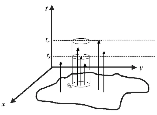
×(tk,tn])is the number of events between times tk and tn, irrespective of their spatial location, and n is the total number of events at that moment (see Figure 2).6.4.4 Iterative calculation of Rn
Every new event requires the recalculation of all n terms in (2). We can decrease substan-tially the amount of numerical calculations by means of an iterative procedure. For k<n, let Ik,n=I(ksn−skk ≤ρ). We have
N(Ck,n+1) =N(Ck,n) +Ik,n+1
and
µ(Ck,n+1) =µ(Ck,n) +µ(B(sk,ρ)×(tn,tn+1]).
Therefore, sinceΛ1,1=1, we can write recursively for k<n+1,
Λk,n+1=Λk,n(1+ε)Ik,n+1 exp(−εµ(B(sk,ρ)×(tn,tn+1])).
By definition,Λn+1,n+1=1 and this completes the recursion.
In practice, to run the procedure, we need ˆµ(Ck,n+1), rather than µ(Ck,n+1). However, this estimated term can also be calculated iteratively for k<n+1:
ˆµ(Ck,n+1) = 1
n+1N(B(sk,ρ)×(0,tn+1])N(
A
×(tk,tn+1])= n+1−k
n+1 N(B(sk,ρ)×(0,tn]) +Ik,n+1
= n
n+1
n−k+1
n−k ˆµ(Ck,n) +
n+1−k n+1 Ik,n+1 = ˆµ(Ck,n) +
k
(n+1)(n−k)ˆµ(Ck,n) +
n+1−k
n+1 Ik,n+1. For k<n+1, we can write
ˆ
Λk,n+1= (1+ε)N(Ck,n)+Ik,n+1 exp −εJn,k
+Λˆn+1,n+1,
where
Jn,k=
n(n−k+1)
(n+1)(n−k)ˆµ(Ck,n) +
Therefore,
Rn+1 = n+1
∑
k=1 ˆ
Λk,n+1
= 1+
n
∑
k=1 ˆ
Λk,nexp
−εk
(n+1)(n−k)ˆµ(Ck,n)
Lε,n,k,
where
Lε,n,k=
(1+ε)exp
−ε n+n+1−1k
Ik,n+1
.
We let 1=Λn+1,n+1=Λˆn+1,n+1. As a consequence, we obtain Rn+1simply by updating the values of ˆΛk,nwith a few numerical calculations.
6.5
Choice of tuning parameters
The variance of the test statistic Rn=∑kΛk,nincreases withεwhen we have no clusters. More importantly, the distribution of Rn is quite asymmetric. Indeed, for one side a large negative deviate of N(Ck,n)from its mean µ(Ck,n)pushΛk,n towards its lower bound, equal to zero. For the other side, increasing a large positive deviate drives Λk,n towards infinity. As a consequence, the false alarm rate increases withε. The simulations in Section 6.6 will show these effects of changingεon the surveillance system performance. Although analytical results are difficult to obtain, simple approximations provide some insight into this trade-off.
When there is no cluster emerging, we have E(Λk,n) =1 for allεbecause
E(Λk,n|H0) = exp(−εµ(Ck,n))E[(1+ε)N(Ck,n)]
= exp(−εµ(Ck,n))exp(µ(Ck,n)(1+ε))exp(−µ(Ck,n))
= 1.
Then, E(Rn) =n for allε, as we could expect from the martingale approach of Section 6.3. Suppose now that a cluster emerges and that N(Ck,n)∼Poisson(µ(Ck,n) (1+ε∗)). At this
They do not need to coincide. In this alternative situation we have
E(Λk,n) = exp(−εµ(Ck,n))E[(1+ε)N(Ck,n)]
= exp(−εµ(Ck,n))exp[µ(Ck,n)(1+ε∗)(1+ε−1)] = exp[µ(Ck,n)εε∗]>1.
That is, E(Λk,n)increases withε(and withε∗).
Therefore, apparently, the choice ofεdoes not affect Rnwhen there is no cluster. When a cluster emerges, choosing a largeε∗will increase Rnand speed up the threshold crossing, as we wish in this case. Hence, it seems that takingε→∞is the a good strategy.
However, there is a penalty for choosingε∗too large in that the Var(Λk,n)increases with
ε∗when there is no cluster. In fact,
Var(Λk,n) =Var[exp(−ε∗µ(Ck,n)) (1+ε∗)N(Ck,n)]
which is equal to
exp(−2ε∗µ(Ck,n)){exp(µ(Ck,n)((1+ε∗)2−1))−exp(2µ(Ck,n)(1+ε∗−1))}.
This reduces to
exp(µ(Ck,n)ε∗2)−1→∞,
asε∗→∞.
Ultimately, this will increase the false alarm rate. Under no cluster, increasing ε∗ too much implies in a larger variability of Rn. This is so because the pairs of terms Λk,n are either uncorrelated (if the corresponding cylinders are non-intersecting) or positively correla-ted (with correlation proportional of the intersecting volume). As a consequence, the variance of the stopping time TA increases as well as the probability that RTA crosses the threshold A
at a very early moment, as well as much later than the expected E(TA) =A. Hence, there is
a larger probability that the threshold will be crossed before any cluster emergence. These effects will be clear in the simulations of Section 6.6.
6.6
Method performance
We evaluated the performance of our method with Monte Carlo simulation using three types of scenarios. In the first type, there were no clusters and the purpose is to evaluate if the approximation A=B≈ARL0 is appropriate. The geographical region was the rectan-gle[0,10]×[0,10] and the spatial location of an event was obtained by independently and uniformly generating coordinates on the square. Times between events were modelled by independent exponential random variables with mean equal to 1. Times and locations were independently generated and henceλ(x,y,t) =0.01. The events were generated sequentially until the alarm was triggered.
In the second type of scenario, in addition to the events generated as in the first scenario, we also simulated events within a cylindrical cluster that emerged at some moment. The purpose of this second type of scenario is to evaluate the detection performance and the effects of the user-specified tuning parameters of our method. The cluster had the square basis[4,5]×[4,5]. It was kept alive from its outbreak until the alarm went off. We selected three different times for the cluster outbreak. In one case, the cluster starts at the beginning of the time period (when t=50) and we label this as case B. In the second case, the cluster starts in the middle of the time period, when t=150, and this is labelled case M. Finally, in the third case, the cylinder cluster starts late, at t=300, and we labelled this as case L.
In each cylinder cluster, we have two types of events: those generated in the larger square and that happened to fall within the cluster, and those events generated within the cluster itself. The intensity at a location (x,y,t) within the cluster is slightly larger than 1.2 times the intensity outside the cluster. This implies that the correct value of the tuning parameter is approximatelyε=0.2.
We will call this second type of scenario as the homogeneous scenario because there is no spatial variation in the events’ intensity except that due to the cluster emergence. The third type of scenario was generated in the same way as the second type except by the use of a spatially heterogeneous density of the events locations. In this third scenario type, the spatial coordinates were generated using a mixture of four bivariate normal distributions. Therefore, at any time, some regions were more likely to observe an event than other regions.
We generated 1000 independent replications of each scenario. To run the surveillance procedure, we used several values for ε: 0.1,0.2,0.4,0.5,2.5,5,10,20. Note that, for the scenario without clusters, the true value of this parameter is zero, while in the scenarios with clusters, it is equal to 0.2.
because it takes too long to run. In each scenario, for a single simulated space time data-set with 1000 events, Kulldorff’s method takes 2 hours and 26 minutes in a machine with 1.66GHz and 1 Gb RAM when we ask for 999 Monte Carlo replications. To repeat this procedure for all the simulated datasets over the many scenarios is unfeasible.
6.6.1 Scenario without clusters
We used the values 50, 100, 200, 300, 400, and 500 for the threshold limit A andρ=1 for the spatial radius of the presumed cluster. If there are no clusters, any surveillance signal is a false signal. If the time period goes to infinity, the statistic Rn will cross the threshold
A with probability one, irrespective of the presence of a real cluster. It is expected that, in a
fixed time period, the number of events until the alarm goes off increases with the increase of the threshold A. If the approximation A=B is reasonable, we should have A≈ARL0.
The graph in Figure 3 shows in the vertical axis the estimated ARL0, the average number of events observed before a false signal is issued, versus the threshold limit A in the horizontal axis. The dashed line represents the line ARL0=A. The other lines represent the test results
for different values ofε.
As we expect, ARL0 increases with the threshold A. Forε=0.1 and 0.2, the approxi-mation ARL0=A is very good. For other values of εthis approximation deteriorates with the increase of A. Initially, the departure from the line ARL0=A is larger the greater is ε. For example, when A=500 andε=0.5, the estimated ARL0is 33% larger than the nominal value of 500. However, the difference between the nominal value A and the true ARL0does not increase monotonically withε. Withε≥10, this difference is almost null. Settingε≥10 is an extreme choice since it means an emerging cluster with intensity 10 times larger than the baseline intensity. It is unlikely that our method is envisioned for such type of anticipated changes.
This result shows that, when no cluster is present and within practical bounds for the expected relative change in intensity, selecting larger values for the user-specifiedεparameter leads to conservative ARL0. That is, if the user is unsure aboutε, selecting a larger value leads to longer ARL0times than the nominal value A.