Available online at www.ispacs.com/jfsva
Volume 2016, Issue 3, Year 2016 Article ID jfsva-00337, 14 Pages doi:10.5899/2016/jfsva-00337
Research Article
Numerical Investigations on Hybrid Fuzzy Fractional
Differential Equations by Improved Fractional Euler Method
D. Vivek1∗, K. Kanagarajan1, S. Harikrishnan1
(1)Department of Mathematics, Sri Ramakrishna Mission Vidyalaya College of Arts and Science, Coimbatore - 641 020, Tamilnadu, India. Copyright 2016 c⃝D. Vivek, K. Kanagarajan and S. Harikrishnan. This is an open access article distributed under the Creative Commons Attribution
License, which permits unrestricted use, distribution, and reproduction in any medium, provided the original work is properly cited.
Abstract
In this paper, the improved Euler method is used for solving hybrid fuzzy fractional differential equations (HFFDE) of orderq∈(0,1)under Caputo-type fuzzy fractional derivatives. This method is based on the fractional Euler method and generalized Taylor’s formula. The accuracy and efficiency of the proposed method is demonstrated by solving numerical examples.
Keywords: Hybrid Fuzzy fractional differential equations, Fractional initial value problems, Caputo-type fuzzy fractional deriva-tive, Improved fractional Euler method.
1 Introduction
The study of fractional differential equations (FDE) forms a suitable setting for mathematical model of real world in various fields viz. Physical and chemical processes. Several forms of FDE have been proposed in more accurate models, and there has been considerable interest in developing numerical methods. M. Mazandarani et.al. proposed the modified fractional Euler method (fuzzy-context) to solve fuzzy fractional differential equations[16, 11].
Hybrid fuzzy differential equations (HFDE) have been focus of many studies due to natural way to model dynamic system with embedded uncertainty[12, 13, 14]. So far, numerical methods have been used to solve these equations such as, Euler method in[12], Runge-Kutta method in[13]. For instance, Pederson et.al[14] investigated the hybrid fractional differential equations.
The aim of this paper is to solve the HFFDE by the improved Euler method under Caputo-type fuzzy fractional deriva-tives. The paper is prepared as follows. After a preliminary section, we will study the Caputo-type fuzzy fractional derivatives. The next section, we discuss HFFDE. Consecutively, we briefly describe the improved fractional Euler method. In the penult section, we present numerical examples to illustrate the theory. Finally in the last section, we give concluding remarks.
2 Preliminaries
We denote byRFthe class of fuzzy subsetsu:R→[0,1]satisfying the following properties:
(a) uis normal, that is, there existx0∈Rwithu(x0) =1.
∗Corresponding author. Email address: peppyvivek@gmail.com, Tel:+919787557676.
(b) uis a convex fuzzy set, that is,
u(λx+ (1−λ)y)≤min{u(x),u(y)}, ∀x,y∈R, ∀λ ∈[0,1].
(c) uis upper semi-continuous onR.
(d) cl{x∈R|u(x)>0}is compact wherecldenotes the closure of a subset.
ThenRFis called the space of fuzzy numbers. For 0<α≤1, set[u]α={s∈R|u(s)≤α}and[u]0={s∈R|u(s)>0}. Then theα-level set[u]αis a non-empty compact interval for all 0≤α≤1 and anyu∈R. The notation[u]α= [uα,uα]
denotes explicitly theα-level set ofu. We refer touanduas the lower and upper branches onurespectively. Foru∈R, we define the length ofuby:len(u) =u−u. Foru,v∈RFandλ∈R, the sumu+vand the productλu are defined by[u+v]α= [u]α+ [v]α,[λu]α=λ[u]α,∀α∈[0,1]where[u]α+ [v]α means the usual addition of two
intervals (subsets) ofRandλ[u]αmeans the usual products between a scalar and a subset ofR. The metric structure is given by the Hausdorff distanced:RF×RF→R+∪{0}defined by
d(u,v) = sup
α∈[0,1]
max{|uα−vα|,|uα−vα|}.
Then it is easy to see thatdis a metric inRF and has the following properties:
(1) d(u+w,v+w) =d(u,v),
(2) d(λu,λv) =|λ|d(u,v),
(3) d(u1+v1,u2+v2)≤d(u1,u2) +d(v1,v2), (4) (RF,d)is a complete metric space, for allu,v,w∈RFandλ∈R.
Definition 2.1. Let x,y∈RF. If there exists z∈RF such that x=y+z then z is called the H-difference of x,y and it
is denoted x⊖y.
Throughtout this paper, the sign⊖always stands for H-difference and we remark that x⊖y≤x+ (−1)y in general. Usually we denote x+ (−1)y by x−y. In the sequel, we fix I= [a,b], for a,b∈R.
Definition 2.2. Let F:I→RFand fix t0∈(a,b). We say that F is (1)-differentiable at t0, if there exists an element
F′(t0)∈RF such that for all h>0sufficiently near to 0 such that F(t0+h)⊖F(t0), F(t0)⊖F(t0−h)and the limits
(in the metric D)
lim h→0+
F(t0+h)⊖F(t0)
h =hlim→0+
F(t0)⊖F(t0−h)
h
=F′(t0) exist.
We say that F is (2)-differentiable if for all h>0sufficently near to 0 such that F(t0)⊖F(t0+h), F(t0−h)⊖F(t0)
and the limits (in the metric D)
lim h→0+
F(t0)⊖F(t0+h) −h =hlim→0+
F(t0−h)⊖F(t0) −h
=F′(t0) exist.
If t0is the end point of I, then we consider the corresponding one-sided derivative.
Theorem 2.1. [11] Let F:[0,∞)→RF. Assume that Fα(x)and F
α
(x)are Riemann-integrable on[a,b]for every b≤a and assume that there are two positive functions Mα, Mαsuch that∫abFα(x)dx≤Mαand∫abFα(x)dx≤Mαfor every b≤a. Then F(x)is improper fuzzy Riemann-integrable on[0,∞)and the improper fuzzy Riemann-integrable is a fuzzy number. Furthermore
[∫ ∞
0
F(x)dx ]α
= [∫ ∞
0
Fα(x)dx,
∫ ∞
0
Fα(x)dx ]
Theorem 2.2. Let F,G:I→RFbe integrable andλ ∈R. Then
(1) ∫I(F(x) +G(x))dx=∫IF(x)dx+∫IG(x)dx
(2) ∫IλF(x)dx=λ∫IF(x)dx
(3) x→d(F(x),G(x))is integrable
(4) d(∫IF(x)dx,∫IG(x)dx)≤∫Id(F(x),G(x))dx.
3 Fuzzy fractional integral and derivative
The space of all continuous fuzzy number valued functions onI, the space of all absolutely continuous fuzzy num-ber valued functions onIand the space of all Lebesgue integrable fuzzy number valued functions onIare respectively denoted byCF(I),(AC)F(I)andLF(I). Throughout this paper, letβ∈(0,1).
Definition 3.1. [5, 16] Let f ∈LF(I). The Riemann-lioville fractional integral of orderβ of the fuzzy number valued function f is defined as follows:
Jaβf(x) = 1 Γ(β)
∫ x
a
f(ε)
(x−ε)1−βdε, x>a,
whereΓ(β)is the well-known Gamma function.
Theorem 3.1. [11] Let f ∈LF(I). The Riemann-Liouville fractional integral of orderβ of the fuzzy number valued function f , based on itsα-cut representation, can be expressed as
[
Jaβf(x)]α=[Jaβfα(x),Jaβfα(x)], x>a,
where
Jaβfα(x) = 1 Γ(β)
∫ x
a
fα(ε)
(x−ε)1−βdε,
Jaβfα(x) = 1 Γ(β)
∫ x
a
fα(ε) (x−ε)1−βdε.
Definition 3.2. [16] If f ∈AC(I), then Riemann-Lioville fractional derivative of orderβ of the crisp function f exists almost everwhere on I and can be represented by
RL
a Dβf(x) = 1 Γ(1−β)
d dx
∫ x
a
f(ε)(x−ε)−βdε.
Note that Riemann-Lioville fractional derivative of orderβ of f is the first order derivative of the fractional integral 1−β of f.
Definition 3.3. [16] If f ∈AC(I), then Caputo fractional derivative of orderβ of the crisp function f exists almost everywhere on I and can be represented by
C
aDβf(x) = 1 Γ(1−β)
∫ x
a
f′(ε)(x−ε)−βdε.
Definition 3.4. [16] Let f∈(AC)F(I)and
G(x) = 1 Γ(1−β)
∫ x
a
f(ε)(x−ε)−βdε, for x>a
If fuzzy number valued function G is (1)-differentiable, then Riemann-Lioville fractional derivative of orderβ of the fuzzy number valued function f exists almost everwhere on I and can be represented byRLa Dβ1f(x) = d
dxG(x). If the
fuzzy number valued function G is (2)-differentiable, then Riemann-Lioville fractional derivative of orderβ of the fuzzy number valued function f exists almost everywhere on I and can be represented byRLa Dβ2f(x) =dxdG(x). Definition 3.5. Let f ∈(AC)F(I). Then f is said to be the Caputo fractional differentiable, fuzzy number valued
function of orderβ at x∈(a,b), if
C
aDβf(x) = 1 Γ(1−β)
∫ x
a
f′(ε)(x−ε)−βdε.
If the fuzzy number valued function f is (1)-differentiable, then f is said to be Caputo differentiable in the first form and denoted byCaDβ1f(x). If f(x)is (2)-differentiable, then f is said to beCaputo differentiable in the second form and denoted byCaDβ2f(x).
Theorem 3.2. Let f ∈(AC)F(I)∩LF(I).[f(x)]α= [fα(x),fα(x)], for x∈(a,b).
(1) If f(x)is Caputo fractional differentiable fuzzy number valued function in the first form, then [
C
aD
β
1f(x) ]α
=[CaDβfα(x),CaDβf
α
(x)].
(2) If f(x)is Caputo fractional differentiable fuzzy number valued function in the second form, then [
C
aD
β
2f(x) ]α
=[C aDβf
α
(x),C
aDβfα(x) ]
.
Theorem 3.3. (Characterization theorem) Let us consider the fuzzy fractional initial value problem {
c
aDβx(t) =f(t,x(t)),
x(t0) =x0,
(3.1)
where f:[t0,t0+a]×E→E is continuous, such that
(A1)|f(t,x)|α=[fα(t,xα,xα),fα(t,xα,xα)],
(A2) xα and xαare continuous and uniformly bounded on any bounded set.
that is for anyε>0there is aδ>0such that
fα(t,x,y)−fα(t,x,y)<εfor allα∈[0,1], whenever(t,x,y),(t1,x1,y1)∈ [t0,t0+a]×R2and∥(t,x,y)−(t1,x1,y1)∥<δ.
(A3) there exists H>0such that
fα(t,x,y)−fα(t1,x1,y1)
≤Hsup{|x2−x1|,|y1−y2|}, ∀α∈[0,1],
then the FFIVP(3.1)and the system of fractional differential equations (FDEs)
c
aDβxα(t) =fα(t,xα,xα), c
aDβxα(t) =f
α
(t,xα,xα),
xα(t0) =xα0,
xα(t0) =xα0
Proof. Assume the hypothesis (A1)-(A3) are satisfied. First fixε>0. Chooseδ=Hε and suppose∥(t,x,y)−(t,x1,y1)∥<
δ. Then,
fα(t,x,y)−fα(t,x1,y1)
≤Hsup{|x1−x|,|y1−y|} ≤H∥(t,x,y)−(t,x1,y1)∥ <Hδ
=ε,
for allα∈[0,1]. Next we must show that fα,fα are uniformly bounded on any bounded set. LetSbe any bounded subset of[t0,t0+a]×R2. Then there exist constantsx1,x2,y1,y2∈Rsuch that ifU= (t,x,y)∈Sthent∈[t0,t0+a],
x∈[x1,x2], andy∈[y1,y2]. Fixα∗∈[0,1]; andU∗∈S. LetK=sup{|t0,t0+a−t0|,|x2−x1|,|y1−y2|}andC=
HK+suppf(U∗), where suppf(U∗)is the support off(U∗). Supposeα∈[0,1]andU∈S. Then,
fα(U)−fα(U∗)≤Hsup{|t0+a−t0|,|x2−x1|,|y2−y1|}, =HK
Also
fα(U)−fα∗(U∗)≤fα(U)−fα(U∗)+fα(U∗)−fα∗(U∗) ≤HK+suppf(U∗)
=C.
Then
fα(U)−fα∗
≤fα(U)−fα∗(U∗)≤C,
nfα(U)≤C+fα∗
Hence, fα is uniformly bounded onS. Similarly, fα is uniformly bounded on any bounded set. Therefore, eqn. (3.1)-(3.2) are equivalent.
Generalized Taylor’s formula under the Caputo-type fuzzy fractional derivative was introdued in[11].
Theorem 3.4. (Generalized Taylor’s formula) Let fe(x)∈(AC)F(I)∩LF(I)and suppose thatc
aDmβef(x)∈CF(I)for
m=0,1,2,3, ...n+1wher0<β<1,0≤x0≤x and x∈(0,b]. then we have [
e
f(x)]α=[fα(x),fα(x)]
fα= n
∑
i=0
xiβ
Γ(iβ+1) c
aDiβfα(0) +
cD(n+1)βfα(x
0) Γ(nβ+β+1) x
(n+1)β
fα= n
∑
i=0
xiβ
Γ(iβ+1) c
aDiβfα(0) +
cD(n+1)βfα(x
0) Γ(nβ+β+1) x
(n+1)β
where,caDβfα(0) =c
aDβfα(x)|x=0,caDβf
α
(0) =c aDβf
α
(x)|x=0.
4 The hybrid fuzzy fractional differential system
Consider the hybrid fuzzy differential system { C
aDβx(t) = f(t,x(t),λm(xm)),t∈[tm,tm+1],m=0,1,2,3...
where{tm}∞m=0, f :[t0,∞)→ ×E×E→E,λm:E→E. Here we assume the existence and uniqueness of solutions of the hybrid system hold on each[tm,tm+1].
To be specific the system would look like:
C
aDβx(t) = C
aDβx0(t) =f(t,x0(t),λ0(x0(t0)))≡f0(t0,x0(t)), x0(t0) =x0, t∈[t0,t1], C
aDβx1(t) =f(t,x1(t),λ1(x1(t1)))≡f1(t1,x1(t)), x1(t1) =x0(t1),t∈[t1,t2], C
aDβx2(t) =f(t,x2(t),λ2(x2(t2)))≡f2(t2,x2(t)), x2(t2) =x1(t2),t∈[t2,t3], .
. . C
aDβxm(t) = f(t,xm(t),λ2(xm(tm)))≡fm(tm,xm(t)), xm(tm) =xm−1(tm),t∈[tm,tm+1], .
. .
(4.4)
Pederson and Sambandham[14] introduced hybrid terms in the fractional differential equations. We note thatβ∈(0,1) andCaDβxmrepresents some type of fractional differentiation(fixed for allm′s). By the solution of Equation (4.3) we mean the following function:
x(t)
x0(t), t0≤t≤t1,
x1(t), t1≤t≤t2,
x2(t), t2≤t≤t3, .
. .
xm(t), tm≤t≤tm+1,
. . .
(4.5)
Theorem 4.1. Consider the FFIVP(3.1)expanded as(3.2)where for m=0,1,2, ...,each fm:[tm,tm+1]×E→E is
such that
(A4)|fm(t,x)|α= [
fα
m(t,x
α,xα),fα
m(t,xα,xα) ]
,
(A5) fα
mand f
α
mare equicontinuous and bounded on any bounded set.
That is, for anyε>0 there is aδm(ε)>0 such that|fmα(t,x,y)−fmα(t1,x1,y1)|<ε for allα ∈[0,1], whenever (t,x,y),(t1,x1,y1)∈[tm,tm+1]×R2and∥(t,x,y)−(t1,x1,y1)∥<δm(ε).
(A6) there exists Hm>0such that
|fmα(t,x1,y1)−fmα(t,x2,y2)| ≤Hksup{|x2−x1|,|y2−y1|} ∀α∈[0,1].
Then,(3.1)and the hybrid system of FDEs c
aDβxαm = fαm(t,xαm(t),xαm(t)), c
aDβxαm = f
α
m(t,xαm(t),xαm(t)),
xαm(tm) =xαm−1(tm) if m>0, xα0(t0) =xα0,
xαm(tm) =xαm−1(tm) if m>0, xα0(t0) =xα0,
(4.6)
Proof. Assume the hypothesis of Theorem 3.3. Suppose x(t) is a solution of eqn.(3.1). Fix m=0,1,2, ...,. If
t∈[tm,tm+1], thenxm(t) =x(t). Sincexm(t)is a solution of the HFFDE
c
aDβxm(t) =fm(t,xm(t)), t∈[tm,tm+1],
xm(tm) = {
xm−1(tm) if m>0
x0(t0) if m=0
(4.7)
and (A4)-(A6) are satisfied,by Theorem 3.3,xαmandxαmsolve (4.6).
Next assume for eachm=0,1,2, ... that xαm(t)andxαm(t)solve (4.6). By Theorem 3.3, xm(t)is a solution of the HFFDE (4.7) for eachm=0,1,2, .... Definex(t)as in (4.5). Then,x(t)is a solution of eqn.(3.1).
For a hybrid fuzzy fractional differential Equation (4.3), we develop the improved fractional Euler’s method via an application for fuzzy fractional differential equations in [11].
The HFFIVP (4.3) is equivalent to the following systems of fractional ordinary differential equations
C
aDβxα(t) = [f(t,x(t),λm(xm))] =F(t,x,x), C
aDβxα(t) = [f(t,x(t),λm(xm))] =G(t,x,x),
xα(0) =xα0, xα(0) =xα0, x∈I.
(4.8)
Numerical method for (4.3) is the same for Caputo-differentiable of the two forms. We assume thatxis Caputo-differentiable of formCaDβx(t).
The initial value problem (4.3) is equivalent to the following integral equations:
xα(t) =JaβF(t,xα,xα) +xα(0),
xα(t) =JaβG(t,xα,xα) +xα(0),
xα=xα0, xα=xα0, t∈I.
(4.9)
Letg(t)be a crisp continuous function and(⌈β⌉)-times differentiable in the independent variabletover the interval of differentiation(integration)[0,b]. Let the interval[0,b]be subdivided intoNsubintervals[tj,tj+1]of step sizeh=Nb using the nodestj=jhfor j=0,1, ....N. Consider the following Riemann-Liouville integral
Jβg(x) = 1 Γ(β)
∫ x
0
g(t)
(x−t)1−βdt t,β∈R+
Making use of the modified trapezoidal rule,Jβg(b) =T(g,h,β)−o(h2), where
T(g,h,β) = ((N−1)β+1−(N−β−1)Nβ
) hβg(0)
Γ(β+2)+
hβg(b) Γ(β+2)
+ N−1
∑
j=1 (
(n−j+1)β+1−2(N−j)β+1+ (N−j−1)β+1) h
βg(t
j) Γ(β+2)
By substitutingt=t1into eqn.(4.9) and approximation of the JβF(t,xα,xα),JβG(t,xα,xα)by the modified trape-zoidalrule withh=t1−t0, we have
x1α(t) =β
hβF(t0,x0α,x0α)
Γ(β+2) +
hβF(t1,x1α,x1α)
Γ(β+2) +x0α
x1α(t) =β
hβG(t0,x0α,x0α)
Γ(β+2) +
hβG(t1,x1α,x1α)
Γ(β+2) +x0α
β ∈(0,1)
(4.10)
wherexjdenotesx(tj). Now, we are going to estimatex1α,x1α by the fractional Euler method. Consider the initial value problems (4.3) and (4.8), supposexe,c
e
x(t)aboutt0=0 and neglect the second order term(involvingh2β), the formula for the fractional Euler method is as follows:
xαj+1=xαj +h
βF(t
j,xjα,xjα)
Γ(β+1) xαj+1=xαj +h
βG(t
j,xjα,xjα)
Γ(β+1) β∈(0,1)
(4.11)
A system of points that approximates the solution ofx(t)is produced by above recursive method. At each step, the fractional Euler method used as a prediction, and the modified trapezoidal rule is used to make a correction to get the finite value. The general formula for the improved fractional Euler algorithm is as follows:
xα(tj) = hβ
Γ(β+2) (
(j−1)β+1−(j−β−1)jβ)F(t0,xα
0,xα0) +Γ(βhβ+2)∑ij=−01
(
(j−i+1)β+1−2(j−i)β+1+ (j−i−1)β+1)F(ti,xα
i ,xαi) + hβ
Γ(β+2)F (
tj,xαj−1+h
βF(t
j−1,xαj−1,xαj−1) Γ(β+1) ,xαj−1+
hβG(tj−1,xαj−1,xαj−1) Γ(β+1)
) +x0
xα(tj) = hβ
Γ(β+2) (
(j−1)β+1−(j−β−1)jβ)G(t0,xα
0,xα0) + hβ
Γ(β+2)∑
j−1 i=0 (
(j−i+1)β+1−2(j−i)β+1+ (j−i−1)β+1)G(ti,xα
i,xαi ) + hβ
Γ(β+2)G (
tj,xαj−1+h
βF(t
j−1,xαj−1,xαj−1) Γ(β+1) ,xαj−1+
hβG(tj−1,xαj−1,xαj−1) Γ(β+1)
) +x0
(4.12)
Theorem 4.2. [14] Consider the systems(4.8)and(4.12). For a fixed k∈Z+and r∈[0,1],
lim h0,....hk→0
xαk,N
k(α) =y
α(t
k+1,α), (4.13)
lim h0,....hk→0
xαk,N
k(α) =y
α(t
k+1,α) (4.14)
Proof. Fixk∈Z+andα∈[0,1]. Chooseε>0. For eachi=0,1, ....,kwe will find aδ∗
i >0 such thathi<δi∗implies
yα(tk+1;α)−xαk,Nk(α)
<εand
yα(tk+1;α)−xαk,Nk(α)
<ε,
where thehivalues are allowable by regular partition of the[ti,ti+1]’s. By convergence of numerical method[15] over [tk,tk+1], there exists aδk∗>0 such that ifhk<δk∗then
zαk,N
k(α)−y
α(t
k+1;α) <ε 2 and zαk,N
k(α)−y
α(t
k+1;α) <ε
2. We may assumeδ∗
k <1. Thenhk<1. By numerical stability there exists aδk>0 such that
zαk,0(α)−xkα,0(α)<δk, and zαk,0(α)−xkα,0(α)<δk (4.15) implies
zαk,N
k(α)−x
α
k,Nk(α)
<ε 2 and zαk,N
k(α)−x
α
k,Nk(α)
<ε
2. Therefore ifhk<δk∗and (4.15) holds then
yα(tk+1;α)−xαk,N
k(α)
≤yα(tk+1;α)−zαk,N
k(α)
+zαk,N
k(α)−x
α
k,Nk(α)
<ε
2+
ε
2=ε, (4.16)
yα(tk+1;α)−xαk,Nk(α)
≤yα(tk+1;α)−zαk,Nk(α)
+zαk,N
k(α)−x
α
k,Nk(α)
<ε
2+
ε
By convergence of the numerical method over[tk−1,tk], there exists aδ∗
k−1>0 such that ifhk−1<δk∗−1then
zαk−1,N
k−1(α)−y
α(tk;α)
<δk/2 and zαk−1,N
k−1(α)−y
α(tk;α)
<δk/2.
zαi,o(α)−yα
i,o(rα)
<δk and
zαi,o(α)−yiα,o(α)<δk. (4.18)
By numerical stability there exists aδk−1>0 such that ifhk−1<δk∗−1then
zαk−1,N
k−1(α)−y
α(tk;α)
<δk/2 and zαk−1,N
k−1(α)−y
α(tk;α)
<δk/2.
Therefore ifhk−1<δk∗−1and (4.18) holds then
yα(tk;α)−xαk−1,N
k−1(α)
≤yα(tk;α)−xαk−1,N
k−1(α)
+zαk−1,N
k−1(α)−x α
k−1,Nk−1(r)
<δk/2+δk/2=δk,
(4.19)
yα(tk;α)−xαk−1,N
k−1(α)
≤yα(tk;α)−xαk−1,N
k−1(α)
+zαk−1,N
k−1(α)−x α
k−1,Nk−1(r)
<δk/2+δk/2=δk,
(4.20)
Continue inductively for eachi=k−2, ...2,1 to find aδi∗>0 such that ifhi<δi∗then
zαi,N
i(α)−y
α(t
i+1;α)
<δi+1/2 and zαi,N
i(α)−y
α(t
i+1;α)
<δi+1/2.
By numerical stability there exists aδi>0 such that
zαi,0(α)−xiα,0(α)<δi, and zαi,0(α)−xiα,0(α)<δi (4.21) implies
zαi,N
i(α)−x
α
i,Ni(α)
<δi+1/2, and zαi,N
i(α)−x
α
i,Ni(α)
<δi+1/2. (4.22)
Therefore ifhi<δi∗and (4.21) holds then
yα(ti+1;α)−xαi,Ni(α)
≤yα(ti+1;α)−zαi,Ni(α)
+zαi,N
i(α)−x
α
i,Ni(α)
<δi+1
2 +
δi+1
2 =δi+1, (4.23)
yα(ti+1;α)−xαi,Ni(α)
≤yα(ti+1;α)−zαi,Ni(α)
+zαi,N
i(α)−x
α
i,Ni(α)
<δi+1
2 +
δi+1
2 =δi+1. (4.24) In particular,there exists aδ1∗>0 such that ifh1<δ1∗and (4.21) holds withi=1 then
yα(t2;α)−xα1,N
i(α)
<δ2 and
yα(t2;α)−xα1,N
i(α)
<δ2
By convergence of the numerical method over[t0,t1], we may chooseδ0∗>0 such thath0<δ0∗implies
yα(t1; 1)−xα0,N 0(α)
<δ1 and
yα(t1; 1)−xα0,N 0(α)
<δ1 (4.25)
5 Numerical Examples
Numerically, Pederson and Sambandam[12, 13] solved some examples in fuzzy context with integer order. To give a clear overview of our study and to illustrate the above discussed method, here and in this section.
Example 5.1. [12] Consider the following HFFIVP { c
D45ex(t) =x(t) +m(t)λk(x(tk)),t∈[tk,tk+1],tk=k, k=0,1,2,3...
e
x(0;r) = [0.75+0.25r,1.125−0.125r],0≤r≤1, (5.26)
where
m(t) = {
2(t(mod1)), if t(mod1)≤0.5 2(1−t(mod1)), if t>0.5,
λk(µ) = { b
0, if k=0
µ, if k∈ {1,2, ...}
The HFFIVP(5.26)is equivalent to the following system of HFFIVP:
cD45ex(t) =x(t),t∈[0,1], e
x0(0;r) = [0.75+0.25r,1.125−0.125r],0≤r≤1, cD45ex
i(t) =xi(t) +m(t)λk(xi(ti)),t∈[ti,ti+1], xi(ti) =xi−1(ti), i=1,2, ....
In(5.26), x(t) +m(t)λk(x(tk))is a continuous function of t,x,andλk(x(tk))and HFFIVP { c
Dqex(t) =x(t) +m(t)λ
k(x(tk)),t∈[tk,tk+1],tk=k, e
x(tk) =xtk,
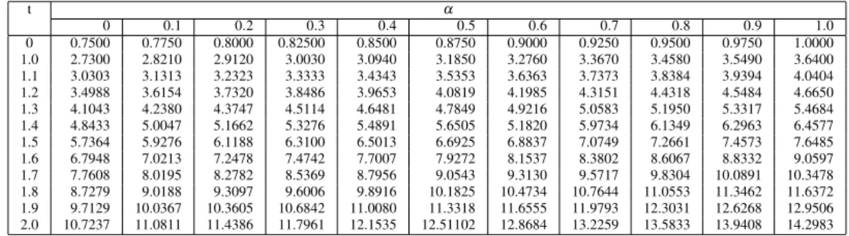
has a unique solution on[tk,tk+1]. To numerically solve the HFFIVP (5.26) we use the improved fractional Euler method for hybrid fuzzy fractional equations the system (5.26). The results are shown in Table 1 and 2.
Furthermore, the approximate solutions in the interval [0,2] are illustrated in Fig.1.
Table 1: The approximate solution to the HFFIVP (5.26)-xα(t)
t α
0 0.1 0.2 0.3 0.4 0.5 0.6 0.7 0.8 0.9 1.0
0 0.7500 0.7750 0.8000 0.82500 0.8500 0.8750 0.9000 0.9250 0.9500 0.9750 1.0000
1.0 2.7300 2.8210 2.9120 3.0030 3.0940 3.1850 3.2760 3.3670 3.4580 3.5490 3.6400
1.1 3.0303 3.1313 3.2323 3.3333 3.4343 3.5353 3.6363 3.7373 3.8384 3.9394 4.0404
1.2 3.4988 3.6154 3.7320 3.8486 3.9653 4.0819 4.1985 4.3151 4.4318 4.5484 4.6650
1.3 4.1043 4.2380 4.3747 4.5114 4.6481 4.7849 4.9216 5.0583 5.1950 5.3317 5.4684
1.4 4.8433 5.0047 5.1662 5.3276 5.4891 5.6505 5.1820 5.9734 6.1349 6.2963 6.4577
1.5 5.7364 5.9276 6.1188 6.3100 6.5013 6.6925 6.8837 7.0749 7.2661 7.4573 7.6485
1.6 6.7948 7.0213 7.2478 7.4742 7.7007 7.9272 8.1537 8.3802 8.6067 8.8332 9.0597
1.7 7.7608 8.0195 8.2782 8.5369 8.7956 9.0543 9.3130 9.5717 9.8304 10.0891 10.3478
1.8 8.7279 9.0188 9.3097 9.6006 9.8916 10.1825 10.4734 10.7644 11.0553 11.3462 11.6372
1.9 9.7129 10.0367 10.3605 10.6842 11.0080 11.3318 11.6555 11.9793 12.3031 12.6268 12.9506 2.0 10.7237 11.0811 11.4386 11.7961 12.1535 12.51102 12.8684 13.2259 13.5833 13.9408 14.2983
Table 2: The approximate solution to the HFFIVP (5.26)-xα(t)
t α
0 0.1 0.2 0.3 0.4 0.5 0.6 0.7 0.8 0.9 1.0
0 1.12500 1.1125 1.1000 1.0875 1.07500 1.0625 1.0500 1.0375 1.0250 1.0125 1.0000
1.0 4.0950 4.0495 4.0040 3.9585 3.9130 3.8675 3.8220 3.7765 3.7310 3.6855 3.6400
1.1 4.5454 4.4949 4.4444 4.3939 4.3434 4.2929 4.2424 4.1919 4.1414 4.0909 4.0404
1.2 5.2482 5.1898 5.1315 5.0732 5.0149 4.9566 4.8983 4.8400 4.7817 4.7233 4.6650
1.3 6.1520 6.0836 6.0153 5.9469 5.8786 5.8102 5.7418 5.6735 5.6051 5.5368 5.4684
1.4 7.2650 7.1842 7.1035 7.0228 6.9421 6.8614 6.7806 6.6999 6.6192 6.5385 6.4577
1.5 8.6046 8.5090 8.4134 8.3178 8.2222 8.1266 8.0310 7.9354 7.8398 7.7441 7.6485
1.6 10.1922 10.0789 9.9657 9.8524 9.7392 9.6259 9.5127 9.3994 9.2862 9.1730 9.0597
1.7 11.6413 11.5119 11.3826 11.2532 11.1239 10.9945 10.8652 10.7358 10.6065 10.4771 10.3478 1.8 13.0918 12.9463 12.8000 12.6554 12.5099 12.3645 12.2190 12.0736 11.9281 11.7826 11.6372 1.9 14.5694 14.4076 14.2457 14.0838 13.9219 13.7600 13.5981 13.4363 13.2744 13.1125 12.9506 2.0 16.0856 15.9068 15.7281 15.5494 15.3706 15.1919 15.0132 14.8344 14.6557 14.4770 14.2983
Example 5.2. Consider the following HFFIVP { c
D0.85ex(t) =x(t) +m(t)λk(x(tk)),t∈[tk,tk+1],tk=k, k=0,1,2,3... e
x(0;r) = [0.75+0.25r,1.125−0.125r], 0≤r≤1, (5.27)
where
m(t) =|sin(πt)|, k=0,1,2..., λk(µ) = { b
0, if k=0
µ, if k∈ {1,2, ...}
Figure 2: The approximate solution to the HFFIVP
Table 3: The approximate solution to the HFFIVP (5.27)-xα(t)
t α
0 0.1 0.2 0.3 0.4 0.5 0.6 0.7 0.8 0.9 1.0
0 0.7500 0.7750 0.8000 0.82500 0.8500 0.8750 0.9000 0.9250 0.9500 0.9750 1.0000
1.0 2.5804 2.6665 2.7525 2.8385 2.9246 3.0106 3.0966 3.1826 3.2686 3.3546 3.4406
1.1 3.0381 3.1394 3.2407 3.3419 3.4432 3.5445 3.6458 3.7471 3.8483 3.9496 4.0508
1.2 3.6387 3.7600 3.8813 4.0026 4.1239 4.2452 4.3665 4.4878 4.0690 4.7303 4.8516
1.3 4.6313 4.5067 4.6521 4.7975 4.9428 5.0881 5.2336 5.3790 5.5243 5.6698 5.1851
1.4 5.1833 5.3561 5.5288 5.7016 5.8744 6.0472 6.220 6.3927 6.5655 6.7383 6.9111
1.5 6.0785 6.2811 6.4838 6.6864 6.8890 7.0917 7.2943 7.4969 7.6995 7.9021 8.1047
1.6 7.0200 7.2540 7.4880 7.7220 7.9560 8.1900 8.4240 8.6580 8.8920 9.1260 9.3600
1.7 7.9828 8.2489 8.5150 8.7811 9.0472 9.3133 9.5794 9.8455 10.1116 10.3777 10.6437
1.8 8.9474 9.2456 9.5439 9.8421 10.1401 10.4386 10.7369 11.0351 11.3333 11.6316 11.9298 1.9 9.9018 10.2319 10.5620 10.8920 11.2221 11.5522 11.8822 12.2123 12.5424 12.8724 13.2025 2.0 10.8443 11.2057 11.5672 11.9288 12.2902 12.6517 13.0131 13.3746 13.7361 14.0976 14.4591
Table 4: The approximate solution to the HFFIVP (5.27)-xα(t)
t α
0 0.1 0.2 0.3 0.4 0.5 0.6 0.7 0.8 0.9 1.0
0 1.12500 1.1125 1.1000 1.0875 1.0750 1.0625 1.0500 1.0375 1.0250 1.0125 1.0000
1.0 3.8707 3.8277 3.7847 3.7417 3.6987 3.6556 3.6126 3.5696 3.5266 3.4836 3.4406
1.1 4.5572 4.5066 4.4559 4.4053 4.3546 4.3040 4.2534 4.2027 4.1521 4.1015 4.0508
1.2 5.4581 5.3974 5.3368 5.2761 5.2155 5.1548 5.0942 5.0335 4.9729 4.9122 4.8516
1.3 6.5420 6.4693 6.3966 6.3239 6.2512 6.1786 6.1059 6.0332 5.9605 5.8878 5.8151
1.4 7.7750 7.6886 7.6022 7.5158 7.4294 7.3430 7.2566 7.1702 7.0839 6.9975 6.9111
1.5 9.1178 9.0116 8.9152 8.8139 8.7126 8.6113 8.5099 8.4086 8.3073 8.2060 8.1047
1.6 10.5300 10.4130 10.2960 10.1790 10.0620 9.9450 9.8280 9.7110 9.5940 9.4770 9.3600
6 Conclusion
In this paper, we utilized the improved fractional Euler method to solve hybrid fuzzy fractional differential equa-tions of orderq∈(0,1). The fractional derivative is considered under Caputo-type fuzzy fractional derivative based on strongly generalized fuzzy differentiability. Consistency, convergence of the numerical method is discussed. The solution obtained using the suggested method and show that this technique can be solved the problem effectively. All numerical results are obtained using Matlab. Higher order methods will be consider in our future work.
Acknowledgements
The authors are grateful to the referees for their careful reading of the manuscript and valuable comments. The authors thank the help from editor too.
References
[1] S. Abbasbandy, T. Allahviranloo, Numerical solutions of fuzzy differential equations by taylor method, Comput. Methods Appl. Math, 2 (2002) 113-124.
http://dx.doi.org/10.2478/cmam-2002-0006
[2] S. Salahshour, T. Allahviranloo, Euler method for solving hybrid fuzzy differential equation, Soft Comput, 15 (2011) 12471253.
http://dx.doi.org/10.1007/s00500-010-0659-y
[3] S. Abbasbandy, T. Allahviranloo, Numerical solution of fuzzy differential equation, Math. Comput. Appl, 7 (2002) 41-52.
http://dx.doi.org/10.3390/mca7010041
[4] S. Abbasbandy, T. Allahviranloo, Numerical solution of fuzzy differential equation by Runge-kutta method, Nonlinear stud, 11 (2004) 117-129.
http://nonlinearstudies.com/index.php/nonlinear/article/view/177
[5] K. Diathelm, N. J. Ford, Freed, Detailed error analysis for a fractional Adams method, Numerical Algorithms, 36 (2004) 31-52.
http://dx.doi.org/10.1023/B:NUMA.0000027736.85078.be
[6] R. Goetschel, W. Voxman, Elementary fuzzy calculus, Fuzzy sets and Systems, 18 (1986) 31-43.
http://dx.doi.org/10.1016/0165-0114(86)90026-6
[7] O. Kaleva, Fuzzy differential equations, Fuzzy Sets and Systems, 24 (1987) 301-317.
http://dx.doi.org/10.1016/0165-0114(87)90029-7
[8] V. Lakshmikantham, X. Z. Liu, Impulsive hybrid systems and stability theory, Internat. J.Nonliear Differential equations, 5 (1999) 9-17.
[9] V. Lakshmikantham, R. N. Mohapatra, Theory of fuzzy differential equations and inclusions, Taylors and Fran-cis, United Kingdom, (2003).
http://dx.doi.org/10.1201/9780203011386
[10] M. Ma, M. Friedman, A. Kandel, Numerical solutions of fuzzy differential equations, Fuzzy Sets and Systems, 105 (1999) 133-138.
http://dx.doi.org/10.1016/S0165-0114(97)00233-9
[11] M. Mazandarani, A. Vahidian Kamyad, Modified fractional Euler method for solving fuzzy fractional initial value problem, Commun. Nonlinear Sci, 18 (2013) 12-21.
[12] S. Pederson, M. Sambandham, Numerical solution of hybrid fuzzy systems, Math Comput. Model, 45 (2007) 1133-1144.
http://dx.doi.org/10.1016/j.mcm.2006.09.014
[13] S. Pederson, M. Sambandham, The Runge-kutta method for hybrid fuzzy differential equations, Nonlinear Anal. Hybrid Syst, 2 (2008) 626-634.
http://dx.doi.org/10.1016/j.nahs.2006.10.013
[14] S. Pederson, M. Sambandham, Numerical solution of hybrid fractional differential equations, Commu. in Ap-plied Anal, 12 (2008) 429-440.
[15] M. Sambandham, Perturbed Lyapunov-like functions and hybrid fuzzy differential equations, Internat.J.Hybrid Syst, 2 (2002) 133-138.
[16] S. Salahshour, T. Allahviranloo et.al; Solving fuzzy fractional differential equations by fuzzy Laplace transform, Commu. Nonlinear Sci Numer. Simulat, 17 (2012) 1372-1381.