ISSN 0101-8205 www.scielo.br/cam
Differential transformation method for solving
one-space-dimensional telegraph equation
B. SOLTANALIZADEH
Young Researchers Club, Sarab Branch, Islamic Azad University, Sarab, Iran
E-mail: [email protected]
Abstract. In this research, the Differential Transformation Method (DTM) has been utilized
to solve the hyperbolic Telegraph equation. This method can be used to obtain the exact solutions
of this equation. In the end, some numerical tests are presented to demonstrate the effectiveness
and efficiency of the proposed method.
Mathematical subject classification: 35Lxx, 35Qxx.
Key words: differential transformation method, spectral method, telegraph equation, Taylor
expansion.
1 Introduction
In this paper we focus on the following one-space-dimensional Telegraph equation:
∂2u ∂t2 +α
∂u
∂t +βu = ∂2u
∂x2 +ψ(x,t) , (1)
whereα, β ∈ R, ψ : R × R → R are known and u : R × R → R is the unknown function. This equation with initial and boundary conditions is con-sidered by some authors. Numerical solution of Telegraph equation with variable coefficient, was discussed in [16]. Mohanty and his coworkers [17, 18], also de-veloped new three-level alternative direction implicit schemes for the two and three-space-dimensional linear hyperbolic equations that these are uncondition-ally stable. Saadatmandi and Dehghan [15], applied a shifted Chebyshev Tau
method. Gao and Chi [22] solved Eq. (1) by a semi-discretization method. They transformed Eq. (1) into a system consisting of ordinary differential equations with respect to time t and then found an exact solution containing an infinite matrix series. Authors of [22], presented two unconditionally stable numerical schemes based onC3 quartic splines with accuracy orders of O(k5+h4)and O(k7+h4).
The concept of DTM was first proposed by Zhou [1], who solved linear and nonlinear problems in electrical circuit problems. Chen and Ho [2] developed this method for partial differential equations. Ayaz [3] applied it to the system of differential equations. During recent years, this method has been used for solv-ing various types of equations by many authors. For example, this method has been used for differential algebraic equations [8], partial differential equations [5, 6, 7], fractional differential equations [10, 11], Volterra integral equations [24] and Difference equations [9]. Shahmorad et al. [19, 20] developed DTM to fractional-order integro-differential equations with nonlocal boundary condi-tions and a class of two-dimensional Volterra integral equacondi-tions. Borhanifar and Abazari applied this method for Burgers and Schrödinger equations [4, 21, 23]. In [14], this method has been utilized for the Kuramoto-Sivashinsky equation with an initial condition. There exist similar problem. For example, authors of [12, 13, 14] presented several matrix formulation method for solving some equation with a boundary integral condition.
The aim of this paper is to extend the differential transformation method to solve the hyperbolic Telegraph equation. The method can be used to evaluate the approximating solution by the finite Taylor series and by an iteration procedure described by the transformed equations obtained from the original equation using the operations of differential transformation.
2 The definitions and operations of DT
2.1 The one-dimensional differential transform
Definition 2.1.If u(t)is analytic in the time domain T then
dku(t)
dtk =ϕ(t,k), ∀t ∈T. (2)
For t = ti, ϕ(t,k) = ϕ(ti,k),wherek belong to the non-negative integer,
denoted as theK domain. Therefore, Eq. (2) can be rewritten as Ui(k)=ϕ(ti,k)=
dku(t)
dtk
t=ti
, ∀t ∈T, (3)
whereUi(k)is called the spectrum ofu(t)att =ti in theK domain. Definition 2.2.If u(t)is analytic, then it can be shown as
u(t)=
∞ X
k=0
(t−ti)k
k! U(k) . (4)
Equation (4) is known as the inverse transformation of U(k). If U(k) is defined as
U(k)=M(k)
dkq(t)u(t) dtk
t=ti
, k=0,1,2, . . . , (5)
then the functionu(t)can be described as
u(t)= 1
q(t) ∞ X
k=0
(t−ti)k k!
U(k)
M(k), (6)
where M(k) 6= 0, q(t) 6= 0. M(k) is called the weighting factor andq(t) is regarded as a kernel corresponding tou(t). If M(k) = 1 andq(t) = 1 then Eqs. (4) and (6) are equivalent. In this paper, the transformation with M(k) =
1/k!andq(t)=1 is applied. Thus from Eq. (7), we have
U(k)= 1
k!
dku(t)
dtk
t=ti
, k =0,1,2, . . . . (7)
obtained by finite-term Taylor series plus a remainder, as
u(t) = 1
q(t)
n
X
k=0
(t−ti)k k!
U(k)
M(k) +Rn+1(t)
=
n
X
k=0
(t−t0)kU(k)+Rn+1(t).
(8)
In order to speed up the convergence rate and improve the accuracy of calcula-tion, the entire domain oftneeds to be split into sub-domains [9, 10].
2.2 The two-dimensional differential transform
Consider a function of two variables w(x,t): R × R → R, and suppose that it can be represented as a product of two single-variable functions, i.e., w(x,t) = u(x)v(t). Based on the properties of one-dimensional differential transform, functionw(x,t)can be represented as
w(x,t)=
∞ X
i=0 ∞ X
j=0
W(i, j)xitj, (9)
whereW(i, j)is called the spectrum of w(x,t). Now we introduce the basic definitions and operations of two-dimensional DT as follows [10].
Definition 2.3. If w(x,t) is analytic and continuously differentiable with re-spect to time t in the domain of interest, then
W(h,k) = 1
k!h!
h ∂k+h
∂xk∂thw(x,t)
i
x=x0,t=t0
, (10)
where the spectrum function W(k,h)is the transformed function, which is also called the T -function. Letw(x,t)as the original function while the uppercase W(k,h) stands for the transformed function. Now we define the differential inverse transform of W(k,h)as following:
w(x,t)=
∞ X
k=0 ∞ X
h=0
Using Eq. (10) in (11), we have w(x,t) =
∞ X
k=0 ∞ X
h=0 1 k!h!
h ∂k+h
∂xk∂thw(x,t)
i
x=x0,t=t0 xkth
=
∞ X
k=0 ∞ X
h=0
W(k,h)xkth.
(12)
wherex0=0 andt0=0.
Now from the above definitions and Eqs. (11) and (12), we can obtain some of the fundamental mathematical operations performed by two-dimensional differential transform in Table 1.
Original function Transformed function
w(x,t)=u(x,t)±v(x,t) W(k,h)=U(k,h)±V(k,h) w(x,t)=cu(x,t) W(k,h)=cU(k,h)
w(x,t)= ∂
∂xu(x,t) W(k,h)=(k+1)U(k+1,h)
w(x,t)= ∂ r+s
∂xr∂tsu(x,t) W(k,h)=
(k+r)!(h+s)!
k!h! U(k+r,h+s)
w(x,t)=u(x,t)v(x,t) W(k,h)= k P
r=0
h P
s=0
U(r,h−s)V(k−r,s)
w(x,t)= ∂
∂xu(x,t)
∂
∂tv(x,t) W(h,k)= k P
r=0
h P
s=0
(k−r+1)(h−s+1)
×U(k−r+1,s)V(r,h−s+1)
Table 1 – Operations of the two-dimensional differential transform.
3 Application of the DTM
In this section, we apply the DTM to solve the presented Telegraph equation. Consider the equation (1),
∂2u ∂t2 +α
∂u
∂t +βu = ∂2u
∂x2 +ψ(x,t), (13)
with the initial conditions
and
∂u(x,0)
∂t =g(x), 0≤x ≤L, (15)
and boundary conditions
u(0,t)=r(t), 0≤t≤ T, (16)
and
u(1,t)=s(t), 0≤t ≤T. (17)
LetU(k,h)as the differential transform ofu(x,t). Applying Table 1, Eq. (2) and Definition 2.3 whenx0 =t0 =0, we get the differential transform version of Eq. (13) as following:
(h+1)(h+2)U(k,h+2)+α(h+1)U(k,h+1)+βU(k,h)
=(k+1)(k+2)U(k+2,h)+ψ(k,h). (18)
By the first initial condition we get ∞
X
k=0
U(k,0)xk =
∞ X
k=0 fk(0)
k! x
k, (19)
which implies
U(k,0)= f
k(0)
k! , k =0,1,2, . . . ,N, (20)
and from the second initial condition and Table 1, we have ∞
X
k=0
U(k,1)xk =
∞ X
k=0 gk(0)
k! x
k, (21)
which implies
U(k,1)= g
k(0)
k! , k =0,1,2, . . . ,N. (22)
Similarly, from the boundary conditions, we have U(0,h)= r
h(0)
h! , h=2,3, . . . ,N, (23)
N
X
k=0
U(h,k)= s
h(0)
Therefore, the values ofU(k,0),U(k,1), and forU(0,h)can be obtained from Eqs. (20), (22) and (23). By using Eqs. (18) and (24), the remainder values of U can be found as follows:
U(k,h+2) = 1
(h+1)(h+2) −βU(k,h)+(k+1)(k+2)U(k+2,h)
−α(h+1)U(k,h+1)+ψ (k,h), k=0,1, . . . ,N−2,
h=0,1, . . . ,N−2.
(25)
Example 3.1. Consider the Eqs. (13)-(15) with the f(x)=x, g(x)= −x r(t)=0, s(t)=exp(−t)
ψ(x,t)=x.exp(−t) α =2, β =2.
Applying Eqs. (20), (22) and (23) in initial and boundary conditions of this problem, we get
U(k,0)=
(
1, fork =1,
0, otherwise, and U(k,1)= (
−1, fork=1,
0, otherwise, and
U(0,h)=0, h=2,3, . . . ,N. From Eqs. (24) and (25), we have
U(0,2) = 1 1×2
−2U(0,0)+(1)(2)U(2,0)−2(0+1)U(0,1)+ϕ(0,0)=0,
U(1,2) = 1 1×2
−2U(1,0)+(2)(3)U(3,0)−2(0+1)U(1,1)+ϕ(1,0)= 1 2!,
U(2,2) = U(3,2)= ∙ ∙ ∙ =0,
U(0,3) = 1 2×3
−2U(0,1)+(1)(2)U(2,1)−2(1+1)U(0,2)+ϕ(0,1)=0,
U(1,3) = 1 2×3
−2U(1,1)+(2)(3)U(3,1)−2(1+1)U(1,2)+ϕ(1,1)= −1 3!,
U(2,3) = U(4,3)= ∙ ∙ ∙ =0, .
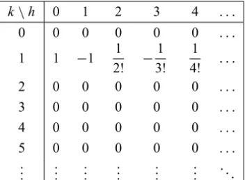
By continuing this process, we obtain
k\h 0 1 2 3 4 . . .
0 0 0 0 0 0 . . .
1 1 −1 1
2! − 1 3!
1 4! . . . 2 0 0 0 0 0 . . .
3 0 0 0 0 0 . . .
4 0 0 0 0 0 . . .
5 0 0 0 0 0 . . . ..
. ... ... ... ... ... . ..
Table 2 – Different obtained values ofU(k,h).
which implies that
u(x,t)≃x
1−t+ 1
2!t
2
− 1
3!t
3
+ ∙ ∙ ∙
which is the Taylor expansion of the
u(x,t)=x×exp(−t) 0≤ x ≤ L,
which is the exact solution of the Example 3.1. The computational results of Example 3.1 are presented in Table 3, and the plot of corresponding exact and approximate functions are shown in Figs. 1 and 2.
(x,t) n=10 n=20
(0,0) 0 0
(0.1,0.6) 8.654×10⁻¹² 6.939×10⁻¹⁸
(0.2,0.9) 1.462×10⁻⁹ 1.387×10⁻¹⁸
(0.3,0.2) 1.665×10⁻¹⁶ 0
(0.4,0.9) 2.924×10⁻⁹ 2.776×10⁻¹⁷
(0.5,0.3) 2.159×10⁻¹⁴ 5.551×10⁻¹⁷
(0.6,0.4) 6.100×10⁻¹³ 1.110×10⁻¹⁶
(0.7,0.4) 7.116×10⁻¹³ 1.110×10⁻¹⁶
(0.8,0.6) 6.924×10⁻¹¹ 5.551×10⁻¹⁷
(0.9,0.7) 4.212×10⁻¹⁰ 0
(1.0,1.0) 2.311×10⁻⁸ 1.110×10⁻¹⁶
0 0.1
0.2 0.3
0.4 0.5
0.6 0.7
0.8 0.9
1
0 0.2 0.4 0.6 0.8 1 0 0.1 0.2 0.3 0.4 0.5 0.6 0.7 0.8 0.9 1
x t
u
(x,
t)
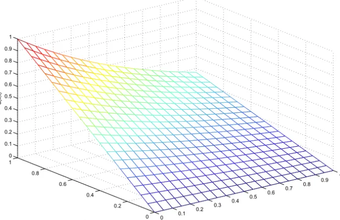
Figure 1 – Plot of exact function from Example 3.1.
0 0.1
0.2 0.3
0.4 0.5
0.6 0.7
0.8 0.9
1
0 0.2 0.4 0.6 0.8 1 0 0.1 0.2 0.3 0.4 0.5 0.6 0.7 0.8 0.9 1
x t
U
(x,
t)
Example 3.2. ([11])Consider the Eqs. (13)-(15) with the f(x)=sin(x), g(x)= −sin(x) r(t)=0, s(t)=sin(1)exp(−t)
ψ (x,t)=0 α=1, β = −1.
From the above initial and boundary conditions and Eqs. (20), (22) and (23), we obtain the corresponding spectra as follows:
U(k,0)=
0, forkis even, (−1)(k−21)
k! , forkis odd,
and
U(k,1)=
0, forkis even, (−1)(k+21)
k! , forkis odd,
and
U(0,h)= r
h(0)
h! , h=2,3, . . . ,N.
From Eqs. (24) and (25), we have U(0,2) = 1
1×2
U(0,0)+(1)(2)U(2,0)−1(0+1)U(0,1)
=0,
U(1,2) = 1 1×2
U(1,0)+(1)(2)U(3,0)−1(0+1)U(1,1)
= 1 2!,
U(2,2) = 1 1×2
U(2,0)+(1)(2)U(4,0)−1(0+1)U(2,1)
=0,
U(3,2) = 1 1×2
U(3,0)+(1)(2)U(5,0)−1(0+1)U(3,1)
= − 1 2!3!,
U(4,2) = 1 1×2
U(4,0)+(1)(2)U(6,0)−1(0+1)U(4,1)
=0,
U(5,2) = 1 1×2
U(5,0)+(1)(2)U(7,0)−1(0+1)U(5,1)
= 1 2!5!,
U(0,3) = 1 2×3
−2U(0,1)+(1)(2)U(2,1)−2(2)(1)U(0,2)=0,
U(1,3) = 1 2×3
−2U(1,1)+(1)(2)U(3,1)−2(2)(1)U(1,2)= −1 3!,
. . .
Thus we get
k\h 0 1 2 3 4 . . .
0 0 0 0 0 0 . . .
1 1 −1 1
2! −
1 3!
1
4! . . .
2 0 0 0 0 0 . . .
3 −1
3! 1 3! −
1 2!3!
1 3!3! −
1 4!3! . . .
4 0 0 0 0 0 . . .
5 1
5! −
1 5!
1 2!5! −
1 3!5!
1
4!5! . . .
..
. ... ... ... ... ... . ..
Table 4 – Different obtained values ofU(k,h).
which implies that
u(x,t) ≃ x
1−t+ 1
2!t
2
− 1
3!t
3
+ ∙ ∙ ∙
+x3
−1
2!+
1 2!t−
1 2!3!t
2
+ 1
2!5!t
3
+ ∙ ∙ ∙
+ ∙ ∙ ∙ ,
which is the Taylor expansion of the
u(x,t)=exp(−t)sin(x),
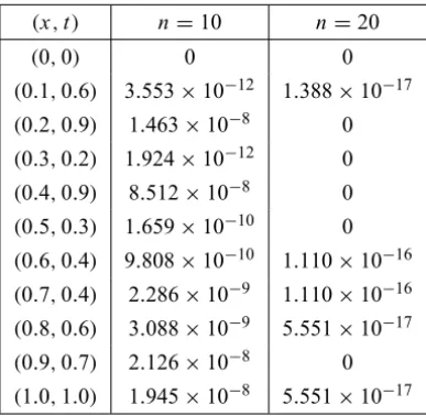
which is the exact solution of the Example 3.2. The computational results of Example 4.2 are presented in Table 5, and the plot of corresponding exact and approximate functions are shown in Figs. 3 and 4.
4 Conclusions
(x,t) n=10 n=20
(0,0) 0 0
(0.1,0.6) 3.553×10⁻¹² 1.388×10⁻¹⁷
(0.2,0.9) 1.463×10⁻⁸ 0
(0.3,0.2) 1.924×10⁻¹² 0
(0.4,0.9) 8.512×10⁻⁸ 0
(0.5,0.3) 1.659×10⁻¹⁰ 0
(0.6,0.4) 9.808×10⁻¹⁰ 1.110×10⁻¹⁶
(0.7,0.4) 2.286×10⁻⁹ 1.110×10⁻¹⁶
(0.8,0.6) 3.088×10⁻⁹ 5.551×10⁻¹⁷
(0.9,0.7) 2.126×10⁻⁸ 0
(1.0,1.0) 1.945×10⁻⁸ 5.551×10⁻¹⁷
Table 5 – Numerical results of Example 3.2.
0 0.1
0.2 0.3
0.4 0.5
0.6 0.7
0.8 0.9
1
0 0.2 0.4 0.6 0.8 1 0 0.1 0.2 0.3 0.4 0.5 0.6 0.7 0.8 0.9
x t
u
(x,
t)
Figure 3 – Plot of exact function from Example 3.2.
0 0.1
0.2 0.3
0.4 0.5
0.6 0.7
0.8 0.9
1
0 0.2 0.4 0.6 0.8 1 0 0.1 0.2 0.3 0.4 0.5 0.6 0.7 0.8 0.9
x t
U
(x,
t)
Figure 4 – Plot of approximate function from Example 3.2 forn=20.
Acknowledgments. The author would like to thank the reviewers for carefully reading the paper and for their constructive comments and suggestions that have improved the paper. The author is deeply grateful to the Young Researchers Club, Sarab Branch, Islamic Azad University, for the financial supports.
REFERENCES
[1] J.K. Zhou, Differential Transformation and Its Applications for Electrical Cir-cuits.Huazhong University Press, Wuhan, China, 1986 (in Chinese).
[2] C.K. Chen and S.H. Ho,Solving partial differential equations by two dimensional differential transform method.Appl. Math. Comput.,106(1999), 171–179.
[3] F. Ayaz,Solutions of the systems of differential equations by differential transform method.Appl. Math. Comput.,147(2004), 547–567.
[5] C.K. Chen, Solving partial differantial equations by two dimensional differential transformation method.Appl. Math. Comput.,106(1999), 171–179.
[6] M.J. Jang and C.K. Chen, Two-dimensional differential transformation method for partial differantial equations.Appl. Math. Comput.,121(2001), 261–270.
[7] F. Kangalgil and F. Ayaz, Solitary wave solutions for the KDV and mKDV equa-tions by differential transformation method.Choas Solitons Fractals,41(2009), 464–472.
[8] J.D. Cole,On a quasilinear parabolic equation occurring in aerodynamics.Quart. Appl. Math.,9(1951), 225–236.
[9] A. Arikoglu and I. Ozkol, Solution of difference equations by using differential transformation method.Appl. Math. Comput.,174(2006), 1216–1228.
[10] S. Momani, Z. Odibat and I. Hashim, Algorithms for nonlinear fractional partial differantial equations: A selection of numerical methods.Topol. Method Nonlin-ear Anal.,31(2008), 211–226.
[11] A. Arikoglu and I. Ozkol, Solution of fractional differential equations by using differential transformation method. Chaos Solitons Fractals, 34 (2007), 1473– 1481.
[12] H.R. Ghehsareh, B. Soltanalizadeh and S. Abbasbandy, A matrix formulation to the wave equation with nonlocal boundary condition. Inter. J. Comput. Math., 88(2011), 1681–1696.
[13] B. Soltanalizadeh, Numerical analysis of the one-dimensional Heat equation subject to a boundary integral specification.Optics Communications,284(2011), 2109–2112.
[14] B. Soltanalizadeh and M. Zarebnia, Numerical analysis of the linear and nonlinear Kuramoto-Sivashinsky equation by using Differential Transformation method.Inter. J. Appl. Math. Mechanics,7(12) (2011), 63–72.
[15] A. Saadatmandi and M. Dehghan, Numerical solution of hyperbolic Telegraph equation using the chebyshev Tau method.Numerical Methods for Partial Differ-ential Equations. doi 10.1002/num.
[16] R. Aloy, M.C. Casaban, L.A. Caudillo-Mata and L. Jodar,Computing the variable coefficient telegraph equation using a discrete eigenfunctions method.Comput. Math. Appl.,54(2007), 448–458.
[18] R.K. Mohanty, M.K. Jain and U. Arora, An unconditionally stable ADI method for the linear hyperbolic equation in three space dimensions. Int. J. Comput. Math.,79(2002), 133–142.
[19] A. Tari, M.Y. Rahimi, S. Shahmoradb and F. Talati,Solving a class of two-di-mensional linear and nonlinear Volterra integral equations by the differential transform method.J. Comput. Appl. Math.,228(2009), 70–76.
[20] D. Nazari and S. Shahmorad,Application of the fractional differential transform method to fractional-order integro-differential equations with nonlocal boundary conditions.J. Comput. Appl. Math.,234(2010), 883–891.
[21] A. Borhanifar and R. Abazari, Exact solutions for non-linear Schrödinger equa-tions by differential transformation method.J. Appl. Math. Comput.,35(2011), 37–51.
[22] F. Gao and C.M. Chi,Unconditionally stable difference schemes for a one-space-dimensional linear hyperbolic equation.Appl. Math. Comput.,187(2007), 1272– 1276.
[23] A. Borhanifar and R. Abazari, Numerical study of nonlinear Schrödinger and coupled Schrödinger equations by differential transformation method. Optics Communications,283(2010), 2026–2031.