An efficient algorithm for some highly nonlinear fractional PDEs in mathematical physics.

An Efficient Algorithm for Some Highly

Nonlinear Fractional PDEs in Mathematical

Physics

Jamshad Ahmad*, Syed Tauseef Mohyud-Din

Department of Mathematics, Faculty of Sciences, HITEC University, Taxila, Pakistan

*jamshadahmadm@gmail.com

Abstract

In this paper, a fractional complex transform (FCT) is used to convert the given fractional partial differential equations (FPDEs) into corresponding partial differential equations (PDEs) and subsequently Reduced Differential Transform Method (RDTM) is applied on the transformed system of linear and nonlinear time-fractional PDEs. The results so obtained are re-stated by making use of inverse transformation which yields it in terms of original variables. It is observed that the proposed algorithm is highly efficient and appropriate for fractional PDEs and hence can be extended to other complex problems of diversified nonlinear nature.

Introduction

Fractional differential equations arise in almost all areas of physics, applied and engineering sciences [1–8]. In order to better understand these physical

phenomena as well as further apply these physical phenomena in practical scientific research, it is important to find their exact solutions. The investigation of exact solution of these equations is interesting and important. In the past several decades, many authors mainly had paid attention to study the solution of such equations by using various developed methods. Recently, the variational iteration method (VIM) [1–3] has been applied to handle various kinds of nonlinear problems, for example, fractional differential equations [4], nonlinear differential equations [5], nonlinear thermo elasticity [6], nonlinear wave equations [7]. In Refs. [8–13] Adomian’s decomposition method (ADM), homotopy perturbation method (HPM), homotopy analysis method (HAM) and variation of parameter method (VPM) are successfully applied to obtain the exact OPEN ACCESS

Citation:Ahmad J, Mohyud-Din ST (2014) An Efficient Algorithm for Some Highly Nonlinear Fractional PDEs in Mathematical Physics. PLoS ONE 9(12): e109127. doi:10.1371/journal.pone. 0109127

Editor:Enrique Hernandez-Lemus, National Institute of Genomic Medicine, Mexico Received:November 26, 2013 Accepted:September 8, 2014 Published:December 19, 2014

Copyright:ß2014 Ahmad, Mohyud-Din. This is an open-access article distributed under the terms of theCreative Commons Attribution License, which permits unrestricted use, distribution, and reproduction in any medium, provided the original author and source are credited.

solution of some highly nonlinear time-fractional partial differential equations of mathematical physics.

Preliminaries

In this section, we give some basic formula and results about fractional calculus, and then we discuss the analysis reduced differential transform method (RDTM) to fractional partial differential equations.

1 Jumarie’s Fractional Derivative

Some useful results and properties of Jumarie’s fractional derivative were summarized [20].

Da_xc~0,a§0,c~constant: ð1Þ

Da_x½c f xð Þ~_{c D}a

xf xð Þ,a§0,c~constant: ð2Þ

Da_xxb~ C 1z_b

ð Þ

Cð1z_b{aÞx

b{a

,b§a§0_: ð3Þ

Da_x½f xð Þg xð Þ~ _Da

xf xð Þg xð Þzf xð Þ D

a

xg xð Þ:

ð4_Þ

Da_xf x t_{ð ð ÞÞ}~f0 xð Þx x

a _t

ð Þ: ð5_Þ

2 Fractional Complex Transform

The fractional complex transform was first proposed [19] and is defined as

T~ p ta

C_ðaz1_Þ X~ q xb

C_ðbz1_Þ Y~ k yc

C_ð1zc_Þ

Z~ l zl

C_ð1zl_Þ 8

> > > > > > > <

> > > > > > > :

: ð6Þ

where p, q,k, and l are unknown constants, 0vaƒ1,0vbƒ1,0vcƒ1,

3 Reduced Differential Transform Method (RDTM)

To demonstrate the basic idea of the DTM, differential transform ofkth_derivative of a function u xð ,tÞ, which is analytic and differentiated continuously in the

domain of interest, is defined as

Ukð Þx ~ 1

k!

Lk_{u x}ð ,tÞ

L_tk

" #

t~t0

, ð7Þ

The differential inverse transform ofUkð Þx is defined as follow

u xð ,tÞ~

X ?

k~0

Ukð Þx ðt{t0Þk, ð8Þ

Eq. (8) is known as the Taylor series expansion ofu xð ,tÞ,aroundt~t0.

Combining Eq. (7) and (8)

u xð ,tÞ~

X ?

k~0 1

k!

Lk_{u x}

,t

ð Þ

L_tk

" #

t~_t0

t{_t0

ð Þk, ð9Þ

when t0~0,above equation reduces to

u xð ,tÞ~

X ?

k~0 1

k!

Lk_{u x}

,t

ð Þ

L_tk

" #

t~_t0

tk, ð10Þ

and Eq. (2) reduces to

u xð ,tÞ~

X ?

k~0

Ukð Þx tk: ð11Þ

Theorem 1:If the original function isu xð ,tÞ~w xð ,tÞzv xð ,tÞ,then the

transformed function is

Ukð Þx ~Wkð Þx zVkð Þx

Theorem 2:Ifu xð ,tÞ~aw xð ,tÞ,then Ukð Þx ~aWkð Þx _:

Theorem 3:Ifu xð ,tÞ~

Lm_{w x}

,t

ð Þ

L_tm ,thenUkð Þx ~

kz_m

ð Þ!

k! Wkð Þx : Theorem 4:Ifu xð ,tÞ~

L_{w x}ð ,tÞ

L_x ,then Ukð Þx ~

L

L_x Wkð Þx :

Theorem 5:Ifu xð ,y,tÞ~

L_{w x}

,y,t

ð Þ

L_x ,then Ukðx,yÞ~

L

Ukðx,y,zÞ~

L

L_x Wkðx,y,zÞ_:

Theorem 7:Ifu xð ,tÞ~x

m_tn_{w x}

,t

ð Þ,thenUkð Þx ~x

m_W

k{nð Þx : Theorem 8:Ifu xð ,tÞ~t

n

,then Ukð Þx ~dðk{nÞ,where

dðk{nÞ~ 1

, k~n

0, k=n

:

Theorem 9:Ifu xð ,tÞ~w

2 x,t

ð Þ,then Ukð Þx ~

Pk

r~0

Wrð Þx Wk{rð Þx :

4 Numerical Applications of RDTM

In this section, we shall apply the reduced differential transform method (RDTM) to construct approximate solutions for some nonlinear fractional PDEs in mathematical physics and then compare approximate solutions to the exact solutions as follows.

4.1 Fornberg-Whitham (FW) Equation [21]

La_u L_ta {

L3_u L_tL_x2 z

L_u L_x zu

L_u L_x ~3

L_u L_x

L2_u L_x2 zu

L3_u

L_x3,0vaƒ1, ð12Þ

with the initial conditions

u xð ,0Þ~e

x

2

: ð13Þ

Applying the transformation [19], we get the following partial differential equation

L_u L_T{

L3_u L_tL_x2 z

L_u L_x zu

L_u L_x ~3

L_u L_x

L2_u L_x2 zu

L3_u

L_x3, ð14Þ

Applying the differential transform to Eq. (14) and Eq. (13), we obtain the following recursive formula

kz1

ð ÞUkz1ð Þx {ðkz1Þ

L2_{Ukz1ð Þx} L_x2 ~ {

L_{Ukð Þx} L_x {

Xk

r~0

Uk{_rð Þx

L_{Urð Þx} L_x

zX

k

r~0

Uk{_rð Þx

L3_{Urð Þx} L_x3 z3

Xk

r~0

Uk{_rð Þx

L2_{Urð Þx} L_x2

ð15_Þ

using the initial condition, we have

U0ð Þx ~e

x

2

: ð16Þ

U1ð Þx ~ { 2

3e x

2

,U2ð Þx ~

2

9e x

2

,U3ð Þx ~ {

4

81e x

2

,_{: :}

The series solution is given by

u xð ,TÞ~e

x

2{ 2

3e x

2_Tz 2

9e x

2_T2{ 4

81e x

2_T3z : : :

The inverse transformation will yields

u xð ,tÞ~e

x 2_{ 2 3e x 2 t a

C_ðaz1_Þ z 2

9e x

2 t 2a

C2_ðaz1_Þ { 4

81e x

2 t 3a

C3_ðaz1_Þz: : : ð17Þ

This solution is convergent to the exact solution [22]

u xð ,tÞ~e

1 2x{

2 3t

: ð18Þ

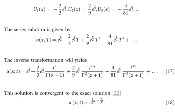
Fig. 1 (a–d): Surface plot of approximate and exact solutions of (12) for different values of a,using only 3

th

order of RDTM solution are:

4.2 Modified Fornberg-Whitham (MFW) Equation [23]

La_u L_ta {

L3_u L_tL_x2 z

L_u L_x zu

2 Lu L_x ~3

L_u L_x

L2_u L_x2 zu

L3_u

L_x3, 0vaƒ1, ð19Þ

with the initial conditions

u xð ,0Þ~

3 4 ffiffiffiffiffi 15 p {5

sec_h2_{ð Þcx} , ð20Þ

where c~ 1

20

ffiffiffiffiffiffiffiffiffiffiffiffiffiffiffiffiffiffiffiffiffiffiffiffiffiffiffiffiffiffi

105{pffiffiffiffiffi15

r

:

Applying the transformation [19], we get the following partial differential equation

L_u L_T{

L3_u L_tL_x2 z

L_u L_x zu

2 Lu L_x ~3

L_u L_x

L2_u L_x2 zu

L3_u

L_x3, ð21Þ

kz1

ð ÞUkz1ð Þx {ðkz1Þ

L2_Ukz1ð Þx

L_x2 ~ {

L_{Ukð Þx}

L_x {

Xk

r~0

Xr

s~

Uk{rð Þx Ur{sð Þx

L_{Usð Þx}

L_x

zX

k

r~0

Uk{rð Þx

L3_{Urð Þx}

L_x3 z3

Xk

r~0

Uk{rð Þx

L2_{Urð Þx}

L_x2

ð22_Þ

using the initial condition, we have

U0ð Þx ~ 3 4 ffiffiffiffiffi 15 p {5

sec_h2_{ð Þ:cx ð}23_Þ

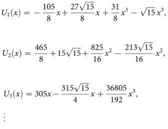
Now, substituting Eq. (21) into (20), we obtain the following values Ukð Þx successively,

U1ð Þx ~ { 105

8 xz 27pffiffiffiffiffi₁₅

8 xz 31

8 x 3

{pffiffiffiffiffi15_x3

,

U2ð Þx ~ 465 8 z15 ffiffiffiffiffi 15 p z 825 16 x 2 {

213pffiffiffiffiffi15

16 x 2

,

U3ð Þx ~305x{

315pffiffiffiffiffi₁₅

4 xz 36805 192 x 3 , .. .

Finally, after applying the inverse transformation the approximate solution is

u xð ,tÞ~

3 4 ffiffiffiffiffi 15 p {5

sec_h2_{ð Þcx} z {

105

8 xz

27pffiffiffiffiffi₁₅

8 xz

31

8 x

3

{pffiffiffiffiffi15_x3

ta

C_ðaz1_Þ

z

465

8 z15

ffiffiffiffiffi 15 p z 825 16 x 2 {

213pffiffiffiffiffi15

16 x

2

t2a

C2_ðaz1_Þz: : :

ð24_Þ

The exact solution [23] of this problem is

u xð ,tÞ~

3 4 ffiffiffiffiffi 15 p {5

sec_h2_{c x} {5{p15ffiffiffiffiffi_t

: ð25Þ

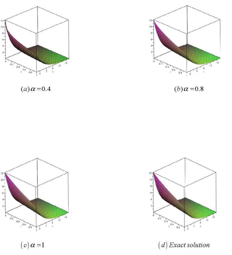
Fig. 2 (a–d): Surface plot of approximate and exact solutions of (19) for different values of a,using only 3

th

Fig. 1. Surface plot of approximate and exact solutions of (12) for different values ofa, using only 3rd order of RDTM solution.

4.3 Sharma-Tasso-Olver (STO) Equation [24]

La_u L_ta z3u

2 Lu L_x z3u

L2_u L_x2 z3

L_u L_x z

L3_u

L_x3 ~0,0vaƒ1, ð26Þ

with the initial conditions

u xð ,0Þ~

1

2 1ztanh x 2

: ð27Þ

Applying the transformation [19], we get the following partial differential equation

L_u L_Tz3u

2 Lu L_x z3u

L2_u L_x2 z3

L_u L_x z

L3_u

L_x3 ~0, ð28Þ

Applying the differential transform to Eq. (28) and (27), we obtain the following recursive formula

kz1

ð ÞUkz1ð Þx ~ {3 Xk

r~0 Xr

s~

Uk{_rð Þx U_r{_sð Þx

L_{Usð Þx} L_x

{3X

k

r~0

Uk{rð Þx L2_U

rð Þx L_x2 {3

L_U sð Þx L_x {

L3_U sð Þx L3_x :

ð29_Þ

using the initial condition, we have

U0ð Þx ~ 1

2 1ztanh x 2

: ð30Þ

Now, substituting Eq. (30) into (29), we obtain the following values Ukð Þx successively,

U1ð Þx ~ { 5

16sech 4 x

2

{ 1

2 coshð Þx sech 4 x

2

,

U2ð Þx ~ { 1

128sech 7

x

2 {18 cosh

x

2 z9cosh

3_x

2 z83 sinh

x

2 {9sinh

3_x

2 z16 sinh 5_x

2

Fig. 2. Surface plot of approximate and exact solutions of (19) for different values ofa, using only 3rd order of RDTM solution.

U3ð Þx ~ { 1

3072

sec_h10x 2

13187{19222cosh_xz5068cosh2_x{718cosh3_xz64cosh4_x

z5184sinh_x{2754sinh2_xz270sinh3_x

!!

,

.. .

The series solution is given by

u xð ,TÞ~

1

2 1ztanh

x 2

{

5

16sech

4x

2{

1

2coshxsech

4x 2 T { 1

128sech

7x

2 {18 cosh

x

2z9cosh

3_x

2 z83 sinh

x

2{9sinh

3_x

2 z16 sinh

5_x

2

T2z

: :

Finally, the inverse transformation will yields the solution

u xð ,tÞ~

1 2 1ztanh x 2 { 5 16sech

4x

2{

1

2coshxsech

4x

2

ta C_ðaz1_Þ

{ 1 128sech

7x

2 {18 cosh

x

2z9cosh 3_x

2 z83 sinh

x

2{9sinh 3_x

2 z16 sinh

5_x 2

t2a

C2_ðaz1_Þz: : :

ð31_Þ

Where the exact solution is

u xð ,tÞ~

1

2 1ztanh x{_t

2

: ð32Þ

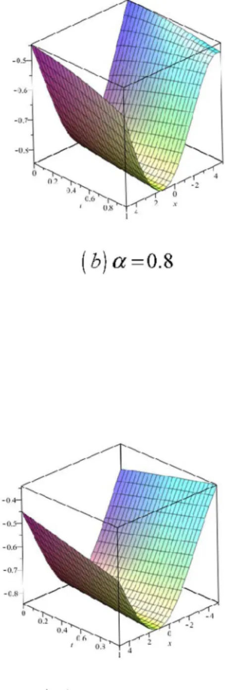
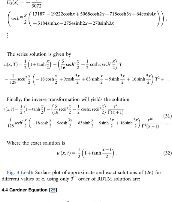
Fig. 3 (a–d): Surface plot of approximate and exact solutions of (26) for different values of a,using only 3

th

order of RDTM solution are:

4.4 Gardner Equation [25]

La_u L_ta {

L3_u L_x3 {6u

2 Lu L_x

{ 6u~0, ð33Þ

with the initial condition

u xð ,0Þ~ {

1 2 1{tanh x 2

: ð34Þ

L_u L_T{

L3_u L_x3 {6u

2 Lu L_x

{ 6_u~0, ð35Þ

Applying the RDTM to (35) and (34), we obtain the recursive relation

kz1

ð ÞUkz1ð Þx {

L3_{Usð Þx}

L3_x {

6X k

r~0 Xr

s~

Uk{rð Þx Ur{sð Þx L_U

sð Þx

L_x {6Usð Þx ~0:

ð36_Þ

using the initial condition, we have

U0ð Þx ~ { 1

2 1{tanh x 2

: ð37Þ

Substituting Eq. (37) into Eq. (36), we obtain the following values Ukð Þx successively,

U1ð Þx ~ { 1

4sech 2 x

2

,

U2ð Þx ~ 1

96sech 2 x

2

27sec_h4 x 2

z27cosh_xsec_h4 x 2

z6sinh 2_{ð Þx} {24sinh_{ð Þx} {108

.. .

The series solution is given by

u xð ,TÞ~ {

1 2 1{tanh x 2 { 1

4sech 2 x

2

Tz 1

96sech 2 x

2

27sec_h4 x 2

z27cosh_xsec_h4 x 2

z6sinh 2_{ð Þx} {24sinh_{ð Þx} {108

T2z : :

Finally, the inverse transformation will yields the solution

u xð ,tÞ~ {

1

2 1{tanh

x 2

{

1

4sech 2 x

2

ta

C_ðaz1_Þz 1

96sech 2 x

2

27sec_h4 x

2

z27cosh_xsec_h4 x

2

z6sinh 2_{ð Þx} {24sinh_{ð Þx} {108

t2a

C2_ðaz1_Þz: : :

Where the exact solution is

u xð ,tÞ~ {

1

2 1{tanh x{t

2

: ð39Þ

Fig. 3. Surface plot of approximate and exact solutions of (26) for different values ofa, using only 3rd order of RDTM solution.

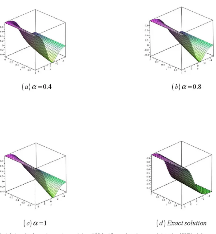
Fig. 4 (a–d): Surface plot of approximate and exact solutions of (33) for different values of a,± using only 3

th

order of RDTM solution are:

4.5 Variant Water Wave (VWW) equation [26]

La_u L_ta z

L_u L_xz

L3_u L_x3 z

L5_u L_x5 {

L

L_x u L2_u

L_x2

~0, ð40Þ

with initial condition

u xð ,0Þ~2{2 tanh

2 ffiffiffiffiffi 10 p x 10

: ð41Þ

Applying the transformation [19], we get the following partial differential equation

L_u L_Tz

L_u L_xz

L3_u L_x3 z

L5_u L_x5 {

L

L_x u L2_u L_x2

~0

, ð42Þ

Applying the RDTM to (42) and (41), we obtain the recursive relation

kz1

ð ÞUkz1ð Þx z L_U

sð Þx L_x z

L3_U sð Þx L_x3 z

L5_U sð Þx L_x5

{ L

L_x

Xk

r~0 Urð Þx

L2_U k{_rð Þx

L_x2 !

~0 :

ð43_Þ

using the initial condition, we have

U0ð Þx ~2{2 tanh 2 ffiffiffiffiffi 10 p x 10

: ð44Þ

Substituting Eq. (44) into (43), we obtain the following values Ukð Þx successively,

U1ð Þx ~ 78 25 ffiffiffi 2 5 r

sec_h2 x{ 39 25t ffiffiffiffiffi 10 p

tanh x{ 39 25t ffiffiffiffiffi 10 p , .. .

The series solution is given by

u xð ,TÞ~2{2 tanh

2 ffiffiffiffiffi 10 p x 10 z 78 25 ffiffiffi 2 5 r

sec_h2 x{ 39 25t ffiffiffiffiffi 10 p

Fig. 4. Surface plot of approximate and exact solutions of (33) for different values ofa, using only 3rd order of RDTM solution.

Fig. 5. Surface plot of approximate and exact solutions of (40) for different values ofa, using only 3rd order of RDTM solution.

Finally, the inverse transformation will yields the solution

u xð ,tÞ~2{2 tanh

2 ffiffiffiffiffi

10 p

x 10

z 78

25

ffiffiffi

2

5

r

sec_h2

x{39_25t

ffiffiffiffiffi

10 p

tanh x{ 39 25t ffiffiffiffiffi

10 p

ta

C_ðaz1_Þz: : :

ð45_Þ

The exact solution [26] is given by

u xð ,tÞ~2{2 tanh

2 ffiffiffiffiffi

10 p

10 x{ 39

25t

: ð46Þ

Fig. 5 (a–d): Surface plot of approximate and exact solutions of (32) for different values of a,using only 3

th _{order of RDTM solution are:}

Conclusions

Applied fractional complex transform (FCT) proved very effective to convert the given fractional partial differential equations (FPDEs) into corresponding partial differential equations (PDEs) and the same is true for its subsequent effect in Reduced Differential Transform Method (RDTM) which was implemented on the transformed system of linear and nonlinear time-fractional PDEs. The solution obtained by Reduced Differential Transform Method (RDTM) is an infinite power series for appropriate initial condition, which can in turn express the exact solutions in a closed form. The results show that the Reduced Differential Transform Method (RDTM) is a powerful mathematical tool for solving partial differential equations with variable coefficients. Computational work fully re-confirms the reliability and efficacy of the proposed algorithm and hence it may be concluded that presented scheme may be applied to a wide range of physical and engineering problems.

Author Contributions

Conceived and designed the experiments: JA SM. Performed the experiments: JA SM. Analyzed the data: JA SM. Contributed reagents/materials/analysis tools: JA SM. Wrote the paper: JA SM.

References

1. Noor MA, Mohyud-Din ST (2008) Modified variational iteration method for heat and wave-like equations. Acta Appl Math 104: 257–269.

3. Abbasbandy S(2007) Numerical solutions of nonlinear Klein-Gordon equation by variational iteration method. Internat J Numer Meth Engrg 70: 876–881.

4. He JH(1999) Some applications of nonlinear fractional differential equations and their approximations. Bull Sci Technol 15: 86–90.

5. Bildik N, Konuralp A(2006) The use of variational iteration method, differential transform method and Adomian decomposition method for solving different types of nonlinear partial differential equation. Int J Non-Linear Sci Numer Simul 7: 65–70.

6. Sweliam NH, Khader MM(2007) Variational iteration method for one dimensional nonlinear thermo-elasticity. Chaos Soliton Fract 32: 145–149.

7. Soliman AA(2006) A numerical simulation and explicit solutions of KdV-Burgers’ and Lax’s seventh-order KdV Equations. Chaos Solitons Fract 29: 294–302.

8. Momani S, Al-Khaled K(2005) Numerical solution for systems of fractional differential equations by the decomposition method. Appl Math Comput 162: 1351–65.

9. Odibat Z, Momani S (2007) Numerical solution of Fokker-Planck equation with space-and time-fractional derivatives. Phys Lett A 369: 349–358.

10. Yıldırım A, Koc¸ak H (2009) Homotopy perturbation method for solving the space-time fractional advection-dispersion equation. Adv Water Resour 32: 1711–1716.

11. Matinfar M, Saeidy M(2010) Application of Homotopy Analysis method to fourth order parabolic partial differential equations. Appl Appl Math 5: 70–80.

12. Mohyud-Din ST, Noor MA, Waheed A(2009) Variation of parameter method for solving sixth-order boundary value problems. Commun Korean Math Soc 24: 605–615.

13. Mohyud-Din ST, Noor MA, Waheed A(2010) Variation of parameter method for initial and boundary value problems. World Appl Sci J 11: 622–639.

14. Jang MJ, Chen CL, Liu YC (2006) Two-dimensional differential transform for partial differential equations. Appl Math Comput 181: 767–774.

15. Arikoglu A, Ozkol I(2007) Solution of fractional differential equations by using differential transform method. Chaos Soliton Fract 34: 1473–1481.

16. Zhou JK(1986) Differential transform and its applications for Electrical Circuits. Huazhong University Press Wuhan, China.

17. Merdan M, Gokdogan A(2011) Solution of nonlinear oscillators with fractional nonlinearities by using the modified differential transformation method. Math Comput Appl 16: 761–772.

18. Kurnaz A, Oturance G (2005) The differential transforms approximation for the system of ordinary differential equations. Int J Comput Math 82: 709–719.

19. Li ZB, He JH(2010) Fractional Complex Transform for Fractional Differential Equations. Math Comput Appl 15: 970–973.

20. Jumarie G (2006) Modified Riemann-Liouville Derivative and Fractional Taylor series of Non-differentiable Functions Further Results. Comput Math Appl 51: 1367–1376.

21. Whitham GB(1967) Variational methods and applications to water wave. Proc R Soc Lond Ser A 299: 6–25.

22. Fornberg B, Whitham GB (1978) A numerical and theoretical study of certain nonlinear wave phenomena. Philos A Trans R Soc Lond Ser A 289: 373–404.

23. He B, Meng Q, Li S(2010) Explicit peakon and solitary wave solutions for the modified Fornberg-Whitham equation. Appl Math Comput 217: 1976–1982.

24. Olver PJ(1977) Evolution equations possessing infinitely many symmetries. Int J Math Phys 18: 1212– 1215.

25. Wazwaz AM(2007) New solitons and kink solutions for the Gardner equation. Comm Nonlin Sci Numer Simul 12: 1395–404.