Available online at www.ispacs.com/cna
Volume 2016, Issue 2, Year 2016 Article ID cna-00245, 23 Pages doi:10.5899/2016/cna-00245
Research Article
Application of Fractional Order Legendre Polynomials: a New
Procedure for Solution of Linear and Nonlinear Fractional
Differential Equations under
m
-point Nonlocal Boundary
Conditions
Hammad Khalil1,2∗, Mohammed Mehdi Rashidi3,4, Rahmat Ali Khan1
(1)Department of Mathematics, University of Malakand, Chakadara Dir(L), Khyber Pakhtunkhwa, Pakistan
(2)University of Poonch Rawlakot, AJK, Pakistan.
(3)Shanghai Key Lab of Vehicle Aerodynamics and Vehicle Thermal Management Systems, Tongji University.
(4)ENN-Tongji Clean Energy Institute of advanced studies, Shanghai, China.
Copyright 2016 c⃝Hammad Khalil, Mohammed Mehdi Rashidi and Rahmat Ali Khan. This is an open access article distributed under the Creative Commons Attribution License, which permits unrestricted use, distribution, and reproduction in any medium, provided the original work is properly cited.
Abstract
In this paper, we have proposed a new formulation for the solution of a general class of fractional differential equa-tions (linear and nonlinear) under ˆm-point boundary conditions. We derive some new operational matrices and based on these operational matrices we develop scheme to approximate solution of the problem. The scheme convert the boundary value problem to a system of easily solvable algebraic equations. We show the applicability of the scheme by solving some test problems. The scheme is computer oriented.
Keywords:Fractional order Legendre polynomials, Fractional differential equations,m-point boundary value problems, Local and nonlocal boundary conditions.
1 Introduction
It is well known that fractional order differential equations provide more accurate results as compare to integer order differential equations. Fractional calculus is generalization of integer order integration and differentiation to its non-integer (fractional) order counterpart. Fractional calculus has proved to be a valuable tool in modeling var-ious phenomena of physics, chemistry, engineering, aerodynamics, electrodynamics of complex medium, polymer rheology, etc. [1-3]. In the last three decades, a tremendous amount of work is devoted to the study of fractional order differential equations and partial differential equations. In most cases it is necessary to solve fractional order differential equations, and the difficulty arise when the system has to be solved under complicated types of boundary conditions. The aim of this paper is to establish a scheme for the approximate solution of fractional order differential equations (linear and non linear) under ˆm-point nonlocal boundary conditions.
ˆ
m-point boundary value problems appear in wave propagation and in elastic stability. For example, the vibrations
of a guy wire of a uniform cross-section, composed ofmsections of different densities can be molded as a m-point boundary value problem ( see [4, 5] and the reference quoted there).
The basic problem to be discussed in this paper is to find the approximate solution of the following classes of fractional differential equations
DσU(t) = n
∑
i=1
biDγiU(t) +b0U(t) +g(t), (1.1)
DσU(t) = n
∑
i=1
bi(t)DγiU(t) +a0(t)U(t) +g(t), (1.2)
DσU(t) + n
∑
i=0
biDγiU(t) =f(U(t),Uγ1(t),Uγ2(t),···Uγn(t)) +g(t), (1.3)
where the order of derivatives are defined asn<σ ≤n+1, 0=γ0<γ1≤1<γ2≤2···γn≤n, t ∈[0,τ] and
g(t)∈C([0,τ])is given source function. In (1.1)biare real constants. bi(t)in (1.2) are coefficients well defined on [0,τ].In (1.3) fis nonlinear function ofU(t)and its fractional derivatives. In the above equationsU(t)is the unknown solution to be determined under the following nonlocal m-point boundary conditions
Ui(0) =ui,i=0,1,···n−1, U(τ) = m−2
∑
i=0
ζiU(ηi). (1.4)
Whereζiare not all equal to zero, andηiare defined as 0<η0<η1···<ηm−2<τ.
To approximate the solution of the above mentioned problems we use Generalized fractional order Legendre polyno-mials. These polynomials are recently applied by Yiming Chen [6] to approximate solution of fractional order partial differential equations with variable coefficients. We develop some new operational matrices and use them along with the matrices developed in [6] to develop a new efficient and simple method to approximate solution of non local boundary value problems. The method we have proposed is a spectral method. Spectral methods are extensively used in the solution of differential equations, function approximation, and variational problems (see, e.g., [7, 8] and the references therein).
Recently spectral method gained attention of many authors. Among others, some of the well known mathematicians who successfully applied spectral method are A. H. Bhrawy [9, 10], E.H. Doha [11-16], A. Saadatmandi [17]. In these papers the authors solved many scientific problems using spectral methods. Actually we are motivated by the work of A. H Bhrawy [18], in which the author solved fractional order differential equations (including linear and nonlin-ear differential equations) with m-point boundary conditions (local) using shifted Legendre polynomials and some collocation technique. The method they proposed can handle local boundary conditions, however nonlocal boundary conditions are difficult to handle. This motivated us to use orthogonal polynomials for the numerical simulation of linear and nonlinear fractional differential equations with m-point nonlocal boundary conditions.
The operational matrices that we introduced has the ability to convert the fractional order non local boundary value problem to a system of easily solvable algebraic equations. The resultant algebraic equations are linear and can be easily solved. Also we introduce the application of operational matrices together with Quasilinearization to solve the nonlinear problems under the same nonlocal boundary value problems.
The Quasilinearization method was introduced by Bellman and Kalaba [19] to solve nonlinear ordinary or partial differential equations as a generalization of the Newton-Raphson method. The origin of this method lies in the theory of dynamic programming. In this method, the nonlinear equations are expressed as a sequence of linear equations and these equations are solved recursively. The main advantage of this method is that it converges monotonically and quadratically to the exact solution of the original equations [20]. Also some other interesting works in which qasi-linearization method is applied to scientific problems are [21-24]. In our previous work we construct some effi-cient methods for the numerical simulation of couple system of fractional differential equations and fractional order partial differential equations [25-35]. In these papers we only solve linear fractional differential equations subject to initial conditions. For the readers, new to the field, we recommend to study our previous work in order to get a better understanding.
Guptta [35] studied the solvability of three point boundary value problem. Since then many researchers are working in this area and provide many useful results which guarantee the solvability and existence of solution of such prob-lems. For interested reader in the existence theory of the problem we refer to study the survey paper presented by Ruyun Ma [36] in which the author presented a detail survey on this topic. In [37] the author showed the existence of positive solution of a general third order multi point boundary value problem. The existence of solution of such types of problems are also discussed by El-Sayed in [38].
The article is organized as follows: In section 2 we recall some definition and basic properties of Generalized frac-tional order Legendre polynomials and approximations theory. In section 3 we derive new operafrac-tional matrices. We also recall some previously derived operational matrices which are helpful in our further investigation. In section 4 the new matrices are used to provide a theoretical treatment to the corresponding problem. In section 5 some test problems are solved.Results are displayed in tables and figures. Finally in the last section a short conclusion is made.
2 Preliminaries and Notation
In this section, we recall some basic definitions and known results from fractional calculus which are important for our further investigation. we refer to [1, 2] for more detail.
Definition 2.1. Given an interval[a,b]⊂R, the Riemann-Liouville fractional order integral of orderσ∈R+of a functionφ∈(L1[a,b],R)is defined by
aItσφ(t) = 1
Γ(σ)
∫ t
a
(t−s)σ−1φ(s)ds, (2.5)
provided the integral on right hand side exists.
Definition 2.2. For a given functionφ(t)∈Cn[a,b], the Caputo fractional order derivative of orderσ is defined as
Dσφ(t) = 1
Γ(n−σ)
∫ t
a
φ(n)(s)
(t−s)σ+1−nds, n−1≤σ<n,n∈N,
provided the right side is point wise defined on(a,∞), where n= [σ] +1in caseσ not an integer and n=σ in case
σis an integer.
Hence, it follows thatIσtk=Γ(Γ(1+1+k+σ)k) tk+σforσ>0,k≥0,DσC=0,for a constantCand
Dσtk= Γ(1+k)
Γ(1+k−σ)t
k−σ, fork≥[σ]. (2.6)
2.1 The Generalized fractional-order Legendre polynomials
The GFL polynomials on the interval[0,τ]is defined as (see for example [6])
Fli(α,τ)(t) = i
∑
k=0 ✵(α,τ)
(i,k) t
kα, i=
0,1,2,3..., (2.7)
where
✵(α,τ) (i,k) =
(−1)i−kΓ(i+k+1)
Γ(i−k+1)Γ(k+1)τkα. (2.8)
The GFL polynomials are orthogonal on the interval[0,τ].
Theorem 2.1. The GFL polynomials are orthogonal on the interval[0,τ]with respect to the weight function wα(t) =
tα−1.Then the orthogonality condition is
∫ τ
0
Fl(αi ,τ)(t)Fl(αj ,τ)(t)wα(t)dt= h
α)
(2i+1)αδi,j. (2.9)
2.2 Function Approximation with GFL polynomials
The orthogonality condition of the GFl polynomials allows us to expand any function f(t)∈L2[0,τ]in terms of GFL polynomials as follows:
v(t) =
∞
∑
i=0
ciFli(α,τ)(t), (2.10)
where the value ofciare obtained by the relation.
ci=
∫ τ
0
v(t)Fli(α,τ)(t)wα(t)dt. (2.11)
In practice we are interested in the truncated series of (2.10), so we can write the infinite series as
v(t)≃vm(t) = m−1
∑
i=0
ciFl(αi ,τ)(t) =KΦ(t), (2.12)
where
K= [c0,c1,···,cm−1], Φ(t) = [Fl0(α,τ)(t),Fl1(α,τ)(t),···,Flm(α−,τ)1(t)]T. (2.13)
Theorem 2.2. Suppose
Diαv(t)∈C[0,τ] f or i=0,1,···,m−1,
and Pαm=Span{Fl(α0 ,τ)(t),Fl1(α,τ)(t),···,Flm(α−,τ)1(t)}.If vm(t) =KΦ(t)is the best approximation to v(t)fromPαm, then the error bound is presented as follows
∥v(t)−vm(t)∥ ≤Γ(mMα+1) √
hα
(2m+1)α. (2.14)
Proof. For the proof of this theorem see [6].
Theorem 2.3. The definite integral of product of three different GFL polynomials and weight function is constant, and the generalized constant is given by relation
∫ τ
0
Fli(α,τ)(t)Fl(αj ,τ)(t)Flk(α,τ)(t)wα(t)dt=Θ(α(i,j,τ),k), (2.15)
where
Θ(α(i,,jτ),k)= i
∑
k=0 j
∑
l=0 r
∑
s=0 ✵(α,τ)
(i,k) ✵ (α,τ) (j,l) ✵
(α,τ) (r,s) k
(α,τ)
(k,l,s). (2.16)
Proof. Consider the expression
∫ τ
0
Fl(αi ,τ)(t)Fl(αj ,τ)(t)Flk(α,τ)(t)wα(t)dt=
∫ τ
0 i
∑
k=0 j
∑
l=0 r
∑
s=0 ✵(α,τ)
(i,k) ✵ (α,τ) (j,l) ✵
(α,τ) (r,s) t
(kα+lα+sα+α−1)dt,
= i
∑
k=0 j
∑
l=0 r
∑
s=0 ✵(α,τ)
(i,k) ✵ (α,τ) (j,l) ✵
(α,τ) (r,s)
∫ τ
0
t(kα+lα+sα+α−1)αdt.
(2.17)
The integral in the above relation derived as
∫ τ
0
t(kα+lα+sα+α−1)αdt= τ
(kα+lα+sα+α)
(kα+lα+sα+α). (2.18) Let
τ(kα+lα+sα+α)
(kα+lα+sα+α)=k
(α,τ)
(k,l,s). (2.19)
Then using (2.19) and (2.18) in (2.17) we get the desire proof.
3 Operational Matrices
In this section we generalize some new operational matrices. These matrices are used to convert the linear and nonlinear fractional differential equations to a system of easily solvable algebraic equations. Some of these proof are also available in different papers, but to make the paper self contained we gave a detail proof of these results.
Lemma 3.1. LetΦ(t)be the function vector as defined in(2.13), then the fractional derivative of orderσofΦ(t)is generalized as
DσΦ(t)≃Z(σ(M,τ)
×M)Φ(t), (3.20)
whereZ(σ(M,τ)
×M)is the operational matrix of derivative of orderσ, and is defined as
Z(σ(M,×τ)M)=
ˆ
△(0,0) △ˆ(0,1) ··· △ˆ(0,m)
ˆ
△(1,0) △ˆ(1,1) ··· △ˆ(1,m) ..
. ... . .. ...
ˆ
△(m,0) △ˆ(m,1) ··· △ˆ(m,m)
. (3.21)
Where the entries are defined as
ˆ
△(i,j)=α(2j+1)τ−σ
i
∑
s=0 j
∑
r=0
✵(j,r)✵ˆ(i,s) Γ(sα+1)
Γ(sα−σ+1)(α(s+r+1)−σ) (3.22)
ˆ ✵(i,s)=
{
0 if sα∈Noand sα<σ;
✵(i,s) if sα∈/Noand sα≥ ⌈σ⌉or sα∈Noand sα≥σ.
Proof. The proof of this lemma is available in [6].
Lemma 3.2. LetΦ(t)be the function vector as defined in(2.13), then the fractional integral of orderσ ofΦ(t)is generalized as
Iσ(Φ(t))≃P(σ( ,τ)
M×M)Φ(t), (3.23)
whereP(σ( ,τ)
M×M)is the operational matrix of integration of orderσ defined by the relation
P(σ(M,×τ)M)=
△(0,0) △(0,1) ··· △(0,m) △(1,0) △(1,1) ··· △(1,m)
..
. ... . .. ...
△(m,0) △(m,1) ··· △(m,m)
, (3.24)
where the entries are defined as
△(i,j)=
i
∑
k=0
α(2j+1)Γ(kα+1)✵(α,τ) (j,l) ✵
(α,τ)
(i,k) τ(kα+lα+σ−1)
(kα+lα+σ+α)Γ(kα+σ+1) . (3.25)
Proof. Consider the general termFli(α,τ)(t), then we may write
IσFli(α,τ)(t) = i
∑
k=0 ✵(α,τ)
(i,k) I
σtkα= i
∑
k=0 ✵(α,τ)
(i,k)
Γ(kα+1)
Γ(kα+σ+1)t kα+σ.
(3.26)
We can write
tkα+σ=
m
∑
j=0 ˆ
where ˆcjcan be easily calculate as
ˆ
cj=
(2j+1)α τα
∫ τ
0
tkα+σ+α−1Fl(αj ,τ)(t)dt. (3.28) which implies that
ˆ
cj=
(2j+1)α τα
j
∑
l=0 ✵(α,τ)
(j,l)
∫ τ
0
tkα+lα+σ+α−1dt= j
∑
l=0
α(2j+1)✵(α,τ) (j,l) τ(
kα+lα+σ−1)
(kα+lα+σ+α) . (3.29)
Using relation (3.29) in (3.26), and after a short simplification we get
IσFli(α,τ)(t) = j
∑
l=0 i
∑
k=0
α(2j+1)Γ(kα+1)✵(α,τ) (j,l) ✵
(α,τ) (i,k) τ(
kα+lα+σ−1)
(kα+lα+σ+α)Γ(kα+σ+1) Fl
(α,τ)
j (t). (3.30)
Using the notation
△(i,j)=
i
∑
k=0
α(2j+1)Γ(kα+1)✵(α,τ) (j,l) ✵
(α,τ)
(i,k) τ(kα+lα+σ−1)
(kα+lα+σ+α)Γ(kα+σ+1) ,
we can also write it in simplified form as
IσFli(α,τ)(t) = j
∑
l=0
△(i,j)Fl(αj ,τ)(t). (3.31)
Evaluating (3.31) fori=0,1···m, j=0,1···mwe get the desire result.
The following two operational matrices are of basic importance in our further analysis.
Lemma 3.3. Let U(t)andφ(t)be any two functions defined in[0,τ], also U(t) =KΦ(t)Then
φ(t)DσY(t) =KR(σ( ,φ)
M×M)Φ(t). (3.32)
WhereR(σ( ,φ)
M×M)is the operational matrix related to functionφ(t)andσ, and is defined as
R(σ( ,φ)
M×M)=Z (σ,τ) (M×M)J
τ,φ
M×M. (3.33)
The matrixZ(σ( ,τ)
M×M)is the operational matrix of derivative as defined in Lemma 3.1 and
JτM,φ×M=
∇0,0 ∇0,1 ··· ∇0,m
∇1,0 ∇1,1 ··· ∇1,m
..
. ... . .. ...
∇m,0 ∇m,1 ··· ∇m,m
, (3.34)
where
∇r,s=
(2s+1)α τα
m
∑
i=0
ciΘα(i,,τr,s).
WhereΘα(i,,rτ,s)is similar as defined in Theorem 2.3, and
ci=
(2i+1)α τα
∫ τ
0
Proof. ConsiderU(t)≃KΦ(t), then by the implication of Lemma 3.1 we can easily write
φ(t)DσU(t) =φ(t)KZ(σ(M,τ)
×M)Φ(t). (3.35)
Now in order to write the product in the form of matrix, we may write
φ(t)DσU(t) =KZ(σ(M,×τ)M)z}|{Φ(t), (3.36) where
z}|{
Φ(t) =[ φ(t)Fl0(α,τ)(t) φ(t)Fl(α1 ,τ)(t) ··· φ(t)Flm(α,τ)(t)
]T
. (3.37)
φ(t)can be easily approximated with GFL polynomials,
φ(t) = m
∑
i=0
ciFli(α,τ)(t), ci=
(2i+1)α τα
∫ τ
0 φ(
t)wα(t)Fli(α,τ)(t)dt. (3.38)
Using (3.38) in (3.37) we may write, (using more generalized notation)
z}|{
Φ(t) =[ ℑ0(t) ℑ1(t) ··· ℑm(t) ]T, (3.39) where
ℑr(t) = m
∑
i=0
ciFli(α,τ)(t)Fl
(α,τ)
r (t),r=0,1···m. (3.40)
Now consider the general termℑr(t), we can approximate it with GFL polynomials as
ℑr(t) = m
∑
s=0
d(r,s)Fl(αr ,τ)(t), (3.41)
whered(r,s)can be calculated using the relation
d(r,s)=(2s+1)α τα
∫ τ
0
ℑr(t)wα(t)Fls(α,τ)(t)dt. (3.42)
Using (3.40) in (3.42) we get
d(r,s)=
(2s+1)α τα
m
∑
i=0
ci
∫ τ
0
wα(t)Fli(α,τ)(t)Flr(α,τ)(t)Fl(αs ,τ)(t)dt. (3.43)
Now using Theorem 2.3 and (3.43) we get
d(r,s)=(2s+1)α τα
m
∑
i=0
ciΘα(i,,rτ,s)=∇(r,s). (3.44)
Now repeating the procedure forr=0,1,···mands=0,1,···mwe can write
ℑ0 ℑ1 .. . ℑm =
∇0,0 ∇0,1 ··· ∇0,m
∇1,0 ∇1,1 ··· ∇1,m ..
. ... . .. ...
∇m,0 ∇m,1 ··· ∇m,m
Fl(α0 ,τ)(t)
Fl(α1 ,τ)(t) .. .
Fl(αm,τ)(t)
. (3.45)
In simplified notation we can write the above equation as
z}|{
Φ(t) =JMτ,φ×MΦ(t). (3.46) Using (3.46) in (3.36) we get
φ(t)DσU(t) =KZ(σ( ,τ)
M×M)J τ,φ
M×MΦ(t). (3.47)
Using the notationR(σ(M,φ) ×M)=Z
(σ,τ) (M×M)J
τ,φ
The operational matrix developed in the previous lemma is of basic importance in the solution of Fractional differential equations(FDEs) with variable coefficients. In solving m-point boundary value problem the following matrix will play important role.
Lemma 3.4. Letφc
n=ctn, where c and n are real constants. Assume U(t) =KΦ(t), then for0<η≤τ
φc
n0IησU(t) =KQ (σ,η,φc
n)
(M×M) Φ(t), (3.48)
whereQ(σ,η,φnc)
(M×M) is operational matrix related toηandφnc,and is defined as
Q(σ,η,φnc)
(M×M) =
d0,0 d0,1 ··· d0,m
d1,0 d1,1 ··· d1,m
..
. ... . .. ...
dm,0 dm,1 ··· dm,m
, (3.49)
where the entries d(i,j)are defined by the relation
d(i,j)=
i
∑
k=0 j
∑
l=0 ✵(α,τ)
(j,l) ✵ (α,τ) (i,k)
cα(2j+1)Γ(1+kα)(ηkα+σ)
ταΓ(1+kα+σ)(lα+α+n)τ
(lα+α+n). (3.50)
Proof. LetU(t) =∑mi=0biFli(α,τ)(t).Then using the definition of fractional integral (2.5)
0IησU(t) =
m
∑
i=0
bi0IησFli(α,τ)(t) = m
∑
i=0
bi i
∑
k=0 ✵(α,τ)
(i,k) 0Iησtkα. (3.51)
By evaluating the integral and simplification we can write
0IησU(t) =
m
∑
i=0
bi( i
∑
k=0 ✵(α,τ)
(i,k)
Γ(1+kα)(ηkα+σ)
Γ(1+kα+σ) ). (3.52)
For simplicity of notation let
z }| { ✵(α,τ,η,σ)
(i,k) =
i
∑
k=0 ✵(α,τ)
(i,k)
Γ(1+kα)(ηkα+σ)
Γ(1+kα+σ) ). (3.53)
Using (3.52) and (3.53) we can write
φnc0IησY(t) =
m
∑
i=0
bi
z }| { ✵(α,τ,η,σ) (i,k) ct
n.
(3.54)
We may also write
z }| { ✵(α,τ,η,σ) (i,k) ct
n= m
∑
j=0
d(i,j)Fl(αj ,τ)(t). (3.55)
Whered(i,j)can be derived as
d(i,j)=cα(2j+1)
z }| { ✵(α,τ,η,σ)
(i,k)
τα
∫ τ
0
tnwα(t)Fl(αj ,τ)(t)dt. (3.56)
Which can be simplified as
d(i,j)=cα(2j+1)
z }| { ✵(α,τ,η,σ)
(i,k)
τα
j
∑
l=0 ✵(α,τ)
(j,l)
∫ τ
0
Or on further simplification we get
d(i,j)=
cα(2j+1)
z }| { ✵(α,τ,η,σ)
(i,k)
τα
j
∑
l=0 ✵(α,τ)
(j,l)
τ(lα+α+n)
(lα+α+n). (3.58)
Using relation (3.53) we get the value ofd(i,j)as
d(i,j)= i
∑
k=0 j
∑
l=0 ✵(α,τ)
(j,l) ✵ (α,τ) (i,k)
cα(2j+1)Γ(1+kα)(ηkα+σ)
ταΓ(1+kα+σ)(lα+α+n)τ
(lα+α+n). (3.59)
Now using (3.55) in (3.54) we may write
φnc0IησU(t) =
m
∑
i=0 m
∑
j=0
bid(i,j)Fl(αj ,τ)(t). (3.60)
Which can be written in matrix form as
φc
n0IησU(t) =KQ (σ,φc
n,η)
(M×M) Φ(t). (3.61)
Where the entries of the matrixQ(σ,φnc,η)
(M×M) are as defined in (3.59). And hence the proof of the lemma is complete.
The matrices derived in this section are of basic importance in the proposed method.
4 Application of the Operational Matrices
Now, we are in the position to state our main result. The operational matrices are used to convert fractional differential equations to system of easily solvable algebraic equations. We gave a detail procedure for solution of three classes of fractional differential equations. These equations are solved subject to ˆm-point boundary conditions.
4.1 Linear Fractional Differential equations
Consider the following linear system of fractional differential equations
DσU(t) = n
∑
i=1
biDγiU(t) +b0U(t) +f(t), 0≤t≤τ, (4.62) subject to nonlocal ˆm-point boundary conditions as
Uj(0) =uj,j=0,1,···n−1, U(τ) = ˆ m−2
∑
i=0
ζiU(ηi), (4.63)
whereζiare all real constant and 0<η1<η2···<ηm−2<τ,∑im=ˆ−02ζiηin−τn̸=0.
We seek the solution of the problem in terms of shifted GFL polynomials such that the following holds.
DγU(t) =KΦ(t). (4.64)
By the application of fractional integral of orderσ, and making use of Lemma 3.2 we get
U(t) =KP((σM,×τ)M)Φ(t) + n
∑
l=0
dltl, (4.65)
wheredn′sare constants of integration. On using then−1 initial conditions we get the firstn−1 constants.
U(t) =KP(σ(M,τ)
×M)Φ(t) + (n−1)
∑
l=0
dnis up to now unknown. Using the ˆm-point boundary condition we get
U(τ) =KP(σ( ,τ)
M×M)Φ(τ) + (n−1)
∑
l=0
ulτl+dnτn, (4.67)
ˆ m−2
∑
i=0
ζiU(ηi) =K
ˆ m−2
∑
i=0 ζiP(σ( ,τ)
M×M)Φ(ηi) +
ˆ m−2
∑
i=0
(n−1)
∑
l=0 ζiulηl
i+dn ˆ m−2
∑
i=0 ζiηn
i. (4.68)
From (4.63), we see that left sides of (4.67) and (4.68) are equal, therefore for the sack to obtain the value ofdn, we can write
{KP(σ( ,τ)
M×M)Φ(τ)−
ˆ m−2
∑
i=0 ζiP(σ( ,τ)
M×M)Φ(ηi)}+{ (n−1)
∑
l=0
ulτl−mˆ−2
∑
i=0
(n−1)
∑
l=0 ζiulηl
i}=dn{ ˆ m−2
∑
i=0 ζiηn
i −τn}. (4.69)
On further simplification we get
dn=K
1 σ1{P
(σ,τ)
(M×M)Ψ(τ)−
ˆ m−2
∑
i=0
ζiP(σ(M,×τ)M)Φ(ηi)}+σ2, σ1̸=0, (4.70)
whereσ1={∑miˆ=−02ζiηin−τn}andσ2= 1
σ1{∑
(n−1)
l=0 ulτl−∑miˆ=−02∑
(n−1)
l=0 ζiulηil}. Now, using (4.70) in (4.66) we get
U(t) =KP(σ( ,τ)
M×M)Φ(t) + (n−1)
∑
l=0
ultl+K
tn
σ1{P
(σ,τ)
(M×M)Φ(τ)−
ˆ m−2
∑
i=0 ζiP
(σ,τ)
(M×M)Φ(ηi)}+σ2t
n.
(4.71)
Now, in view of Lemma 3.4 we can write (4.71) as
U(t) =KP(σ( ,τ)
M×M)Φ(t) +K{Q (σ,φn
c0,τ)
(M×M) −
m−2
∑
i=0
Q(σ,θ
n ei,ηi)
(M×M) }Φ(t) +F1Φ(t), (4.72)
where∑(l=n−01)ultl+σ2tn=F
1Φ(t),φc0n = t
n
σ1,c0= 1
σ1,θ n ei=ζi
tn
σ1,ei=
ζi
σ1. On further simplification we can write
U(t) =Kz}|{S Φ(t) +F1Φ(t). (4.73) Wherez}|{S =P(σ( ,τ)
M×M)+{Q (σ,φn
c0,τ)
(M×M) −∑
m−2 i=0 Q
(σ,θn ei,ηi)
(M×M) }.Now using (4.73) and Lemma 3.1 we may write
n
∑
j=1
bjDγjU(t) =K
z}|{ S
n
∑
j=1
bjZ
(γj,τ)
(M×M)Φ(t) +F1
n
∑
j=1
bjZ
(γj,τ)
(M×M)Φ(t). (4.74)
Using (4.74),(4.73) and (4.64) in (4.62) we can write
KΦ(t) =Kz}|{S
n
∑
j=1
bjZ
(γj,τ)
(M×M)Φ(t) +b0K z}|{
S Φ(t) +F1 n
∑
j=0
bjZ
(γj,τ)
(M×M)Φ(t) +F2Φ(t). (4.75)
whereF2Φ(t) =f(t). On further simplification we can write {K−K(z}|{S
n
∑
j=1
bjZ
(γj,τ)
(M×M)−b0
z}|{
S )−F2−F1 n
∑
j=0
bjZ
(γj,τ)
(M×M)}Φ(t) =0. (4.76)
Or
{K−K(z}|{S
n
∑
j=1
bjZ
(γj,τ)
(M×M)−b0
z}|{
S )−F2−F1 n
∑
j=0
bjZ
(γj,τ)
(M×M)}=0. (4.77)
4.2 FDEs with variable coefficients
Consider the following class of fractional order differential equations
DσV(t) = n
∑
j=1
bj(t)DγjV(t) +b0(t)V(t) +g(t), 0≤t≤τ. (4.78)
With the following m-point conditions
Vj(0) =vj,j=0,1,···n−1, V(τ) = ˆ m−2
∑
i=0
ζiV(ηi), (4.79)
whereζiare all real constant and 0<η1<η2···<ηm−2<τ,∑im=ˆ−02ζiηin−τn̸=0. As in the previous part assume
DσV(t) =KΦ(t). (4.80)
Then repeating the same steps as in the previous section from (4.64) to (4.73) we get
V(t) =Kz}|{S Φ(t) +F1Φ(t). (4.81) Herez}|{S is defined analogously as in previous section. Now, using (4.81) and Lemma 3.3 we can write
n
∑
j=1
bj(t)DγjV(t) =Kz}|{S
n
∑
j=1
R(γj,bj)
(M×M)Φ(t) +F1R (γj,bj)
(M×M)Φ(t),
b0(t)V(t) =Kz}|{S R(0,b0)
(M×M)Φ(t) +F1R( 0,b0)
(M×M)Φ(t).
(4.82)
Using (4.82) and (4.80) in (4.78) we get
KΦ(t) =Kz}|{S
n
∑
j=0
R(γ( j,bj)
M×M)Φ(t) +F1
n
∑
j=0
R(γ( j,bj)
M×M)Φ(t) +F2Φ(t). (4.83)
After simplification and cancelling out the common term as in previous part we can get system of algebraic equations as
K−Kz}|{S
n
∑
i=0
R(γi,bi)
(M×M)−F1
n
∑
i=0
R(γi,bi)
(M×M)−F2=0. (4.84)
Equation (4.84) is system of easily solvable matrix equation. Which can easily solved for the unknownK. Using the value ofKin (4.81) will lead us to the approximate solution of the problem.
4.3 Non linear FDEs with m-point boundary conditions
The nonlinear fractional order differential equations can be solved by using operational matrix method combined with qasilinearization method. The general procedure of qasilinearization method is as given in the following steps.
• Solve the linear part of nonlinear differential equations under the ˆm−point nonlocal boundary conditions using the method developed in section 4.1. And label the solution of this linear part asUo(t).
• Linearize the nonlinear part of the differential equation atUo(t)with the help of multivariate Taylor series expansion, the linearized equation is now a linear differential equation with variable equation. Solve this lin-earized equation by the method developed in section 4.2. Label the solution asU1(t), and is the solution of the nonlinear problem at first iteration.
• The solution of the qasilinearization method converges to the exact solution of the problem in the sense that the difference between any two consecutive solution becomes smaller and smaller as we proceed the iteration.
The whole process can be seen as a recurrence relation. Consider the following nonlinear fractional differential equation.
DσU(t) + n
∑
j=1
biDγiU(t) =f(U(t),Uγ1(t),Uγ2(t),···Uγn(t)) +g(t). (4.85)
First solve the linear part under the given nonlocal conditions
DσU(t) + n
∑
j=1
bjDγjU(t) =g(t). (4.86)
This equation can be easily solved using the method developed in section 4.1.The solution of this part is labelled as
U0(t).The next step is to linearize the nonlinear part with multi variate Taylor series expansion. So after linearizing and simplification we get
DσU(1)(t) +
n
∑
j=0
bjDγjU(1)(t) =f((U(0)(t),U(γ01)(t),U γ2
(0)(t),···U γn
(0)(t))
+ n
∑
j=0
(U(γ1j)−Uγi
(0))
∂f
∂Uγj(U(0)(t),U
γ1
(0)(t),U γ2
(0)(t),···U γn
(0)(t)) +g(t).
(4.87)
The above equation is a fractional order differential equation with variable coefficients. And can be easily solved with the method developed in section 4.2. The solution at this stage will be labelled asU1(t)and is the solution of the problem at first iteration. Again we have to linearize the problem aboutU1(t)to obtain the solution at second iteration. The whole process can be seen as a recurrence relation like
DσU(r+1)(t) +
n
∑
j=0
bj(t)DγjU
(r+1)(t) = z}|{
F(t). (4.88)
And the boundary conditions becomes
Urj+1(0) =uj,Ur+1(τ) =
ˆ m−2
∑
i=0
ζiUr+1(ηi),
wherebj(t) =bj−∂∂Ufγj(U(r)(t),U(γr1)(t),U γ2
(r)(t),···U γn
(r)(t))and
z}|{
F(t) = f((U(r)(t),Uγ1
(r)(t),U γ2
(r)(t),···U γn
(r)(t))−
n
∑
j=0
U(γrj) ∂f
∂Uγj +g(t).
It can be easily noted that (4.88) is fractional differential equation with variable coefficients.Using the initial solution
X0(t)we may start the ittertions.The coefficientsci(t)and the source termz}|{F(t)can be updated at every iterationrto get the next solution atr+1. At every step we may solve the problem at given nonlocal boundary conditions.
5 Test Problem
In order to show the efficiency of the method we solve some test problems whose exact solution in known . The results are displayed graphically. We solve the problems with different scale level. To show the accuracy of the method we measure the absolute difference of exact and approximate solution. The following notation is used in the
Example 5.1. Consider the following fractional order three point boundary value problems [40].
D32U(t) +e
−3π √
π U(t) =g(t), t∈[0,1],
U(0) =0, U(1) =−125 196 U(
2 5).
(5.89)
Where the forcing term g(t)is defined as
g(t) =e− 3π √
π (t
2(40t2−74t+33) +4e3π√t(128t2−148t+33)). (5.90)
The exact solution of this problem is
U(t) =t5−37t
3 20 +
33t2
40 . (5.91)
For this problem we haveτ=1,η=2
5,n=2,ζ=− 125
196 .To be simple, for this problem we fixα=1,M=7. We first assume solution such that
D32U(t) =KΦ(t). (5.92)
Now application of integral of order32we get
U(t) =KP(
3 2,1)
(7×7)Φ(t) +c0+c1t. (5.93)
We calculateP(
3 2,1)
(7×7)using the procedure given in the above lemmas and is given as
P(
3 2,1)
(7×7)=
0.3009 0.3869 0.0716 −0.0091 0.0027 −0.0011 0.0005 −0.1290 −0.1003 0.0586 0.0231 −0.0039 0.0014 −0.0006
0.0143 −0.0352 −0.0386 0.0274 0.0123 −0.0023 0.0008 0.0013 0.0099 −0.0195 −0.0222 0.0167 0.0078 −0.0015 0.0003 0.0013 0.0068 −0.0130 −0.0150 0.0115 0.0056 0.0001 0.0004 0.0010 0.0050 −0.0094 −0.0110 0.0086 0.0000 0.0001 0.0003 0.0008 0.0039 −0.0072 −0.0085
. (5.94)
Using the initial conditionU(0) =0 implies thatc0=0,however for calculation ofc1we use conditionsU(1) =
−125 196U(
2
5).We can write
U(1) =KP(
3 2,1)
(7×7)Φ(1) +c1, (5.95)
and
U(2
5) =KP
(3 2,1)
(7×7)Φ(
2 5) +c1
2
5. (5.96)
From the equality of (5.95) and (5.96) we can findc1as
c1=−
3 5KP
(3 2,1)
(7×7)Φ(1) +
3 5KP
(3 2,1)
(7×7)Φ(
2
5). (5.97)
Using the value ofc0andc1in (5.95), we can write
U(t) =KP(
3 2,1)
(7×7)Φ(t)−
3t
5KP
(3 2,1)
(7×7)Φ(1) +
3t
5KP
(3 2,1)
(7×7)Φ(
2
5). (5.98)
In view of Lemma 3.4 we can write (5.98) as
U(t) =KP(
3 2,1)
(7×7)Φ(t)−KQ (3/2,θ1
3/5,1)
(7×7) Φ(t) +KQ (3/2,θ1
−3/5,2/5)
where the matricesQ(3/2,θ
1 3/5,1)
(7×7) andQ (3/2,θ1
−3/5,2/5)
(7×7) can be calculated as
Q(3/2,θ
1 3/5,1)
(7×7) =
0.2257 0.2257 0 0 0 0 0 −0.0451 −0.0451 0 0 0 0 0 −0.0064 −0.0064 0 0 0 0 0 −0.0021 −0.0021 0 0 0 0 0 −0.0010 −0.0010 0 0 0 0 0 −0.0005 −0.0005 0 0 0 0 0 −0.0003 −0.0003 0 0 0 0 0
, (5.100)
Q(3/2,θ
1 −3/5,2/5)
(7×7) =−
0.0571 0.0571 0 0 0 0 0 −0.0388 −0.0388 0 0 0 0 0 0.0148 0.0148 0 0 0 0 0 0.0010 0.0010 0 0 0 0 0 −0.0043 −0.0043 0 0 0 0 0 0.0008 0.0008 0 0 0 0 0 0.0018 0.0018 0 0 0 0 0
. (5.101)
After simplification we get
U(t) =KS(7×7)Φ(t), (5.102) where
S(7×7)=P(
3 2,1)
(7×7)−Q (3/2,θ1
3/5,1)
(7×7) +Q (3/2,θ1
−3/5,2/5)
(7×7) . (5.103)
From above equation we calculateS(7×7)as
S(7×7)=
0.0181 0.1041 0.0716 −0.0091 0.0027 −0.0011 0.0005 −0.0450 −0.0163 0.0586 0.0231 −0.0039 0.0014 −0.0006
0.0060 −0.0435 −0.0386 0.0274 0.0123 −0.0023 0.0008 0.0024 0.0110 −0.0195 −0.0222 0.0167 0.0078 −0.0015 0.0056 0.0066 0.0068 −0.0130 −0.0150 0.0115 0.0056 −0.0002 0.0001 0.0010 0.0050 −0.0094 −0.0110 0.0086 −0.0014 −0.0013 0.0003 0.0008 0.0039 −0.0072 −0.0085
. (5.104)
Now using (5.102) and (5.92) in (5.89), we get the following system of matrix equation
KΦ(t) +e− 3π √
π KS(7×7)Φ(t) =GΦ(t), (5.105) whereGis the approximation of source term and we found it to be
G= [0.1938 0.8272 1.8331 0.9695 −0.0190 0.0402 −0.0279]T. (5.106)
(5.105) can be simplified and the unknownKcan be calculated as
K= (I−e−
3π √
π S(7×7))
(−1)G. (5.107)
We get
K= [0.1938 0.8272 1.8330 0.9695 −0.0190 0.0402 −0.0279].
On using the value ofKin (5.102) we get the approximate solution at scale levelM=7 as
Table 1: Comparison of absolute error of Example 5.1 obtained with proposed method(PM) and its comparison with absolute error obtained using Haar wavelets reported in [40].
M=8 (HW) M=7 (PM) M=16 (HW) M=14(PM) M=32(HW) M=25 (PM) t=0.1 6.973(−5) 4.1924(−6) 2.871(−6) 2.2120(−6) 4.426(−7) 6.0500(−9) t=0.2 4.592(−5) 2.1388(−5) 7.082(−6) 2.4057(−6 1.786(−7) 3.1565(−9) t=0.3 4.592(−5) 1.4791(−5) 7.082(−6) 3.7043(−6) 1.800(−7) 1.0438(−9) t=0.4 1.133(−4) 4.4555(−6) 2.869(−6) 1.3128(−6) 4.422(−7) 4.0409(−9) t=0.5 1.373(−4) 2.2802(−5) 8.583(−6) 3.9233(−6) 5.358(−7) 6.1006(−9) t=0.6 1.133(−4) 9.5565(−6) 2.870(−6) 1.0840(−7) 4.418(−7) 7.9848(−9) t=0.7 5.800(−5) 1.0924(−5) 7.080(−6) 4.0054(−6) 1.782(−7) 1.8091(−9) t=0.8 6.679(−5) 1.3612(−5) 7.079(−6) 5.2542(−7) 1.781(−7) 8.8290(−9) t=0.9 6.275(−4) 1.5043(−5) 4.172(−6) 4.8322(−6) 4.408(−7) 1.3494(−8)
In [40] this problem is solved using Haar Wavelets. We compare our results with the results obtained using Haar wavelets. We observe that the absolute error using proposed method is accurate as compare to Haar wavelets. For example the maximum error obtained withM=8 is 1.133×10⁻⁴, while the proposed method yields maximum error 1.0924×10⁻⁵at scale level M=7. Also the proposed method produce more accurate solution atM=20 than that obtained with Haar wavelets atM=32,see Table 1.
Note: The above calculation is obtained using computational software MatLab, and maybe the results are more accurate by simulating the algorithm using more powerful softwares.
Example 5.2. Consider the following 7-point nonlocal boundary value problem.
D2.5U(t) =D2U(t) +2DU(t) +3U(t) +g(t),
U(0) =− 2 100,U
′(0) = 2
100, 1
10U(1) + 5 100U(
11 8 ) +
81 100U(
14 8 )−5U(
17 8 ) +
327 100U(
20
8 ) =U(3).
(5.109)
We select g(t)such that the exact solution of the problem is known. For this problem we consider g(t)as
g(t) =
(
t−29
10
)5(
23 5 +
t4 5 +
3t5 50
)
+
(
t−29
10
)4( t4+t
5 5
)
+
(
t−29
10
)3(
2t5 5
)
− (
t−29
10
)2(
1 25+
2t
25+ 3t2
50
) −
(
2t−29
5 ) ( 2t 25+ t2 25 ) −3t
50− t2 25+ 1 50 +5081767996463981 9007199254740992( √
t(−32768t 7 3575 +
356352t6
3575 −
1722368t5
4125 +
1560896t4
1875 −
16974744t3
21875 + 20511149t2
78125 + 16t
25 − 174 125)).
The exact solution of this problem under the above condition is
U= t
50+
t2(t−29 10
)2 50 −
t5(t−29 10
)5 50 −
1 50.
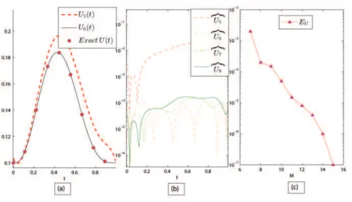
We approximate the solution of this problem with different scale level. As shown in Fig1(a) as the scale level increases
solution matches very well. One can also see in Fig2(b) that the absolute difference decrease with the increase in
scale level. It can be easily noted from this figure that the absolute amount of difference is much more less than10−4,
which is acceptable number. To show that the method is convergent we calculate the quantity EU at different scale
level and observe that the method is highly convergent. This phenomena can be seen in Fig1(c), where EU is plotted
verses scale level M.
Figure 1: (a) The comparison of approximate solution with exact solution of example 5.2 at different scale levels. (b) Absolute error at different scale levels. (c)EU vsM, convergence of the scheme.
Example 5.3. Consider the following 8-point nonlocal boundary value problem.
D3U(t) =3.6D2U(t) +2.4DU(t) +1.5U(t) +g(t),
U(0) =10,U′(0) =−10,
1 10U(
1 4) +
5 10U(
13 36) +U(
17 36) +
12 10U(
21 36) +
15 10U(
25 36)−
53 10U(
29
36) =U(1).
(5.110)
We select
g(t) =−75
(
200t3−260t2+902t+893) (10t+1)4 .
The exact solution of this problem is U(t) = 1
t+101 .We solve this problem with the proposed method.We found that
the method works well, and the approximate solution is in good agreement with the exact solution. The results of
this problem are displayed in Fig2. In Fig2(a), the comparison of exact solution with the approximate solution at
different scale levels is displayed. In Fig2(b) the absolute error is displayed at scale levels ranging from 4 to 16. We
observed that the absolute error decrease with increasing of scale level. We also calculate the quantity EU for this
Figure 2: (a) The comparison of approximate solution with exact solution of example 5.3 at different scale levels. (b) Absolute error at different scale levels. (c)EU vsM, convergence of the scheme.
Example 5.4. Consider the following 6-point nonlocal boundary value problem.
D2.5U(t) = (t3−t2+2)D1.8U(t) + (t2+1)D.8U(t) +tU(t) +g(t),
U(0) =1/10,U′(0) =0,
U(1
2) + 15 10U(
5 8) +U(
6 8)−
41 10U(
7
8) =U(1).
(5.111)
Consider
g(t) =25408839982319905 √
t(896t4−2304t3+2016t2−672t+63) 23643898043695104 −t
(
10t3(t−1)4+ 1 10
) −
445907303348948125 203274472780994707456t
11
5 (t2+1) (21875t4−77500t3+100750t2−56420t+11284) − 89181460669789625
6557241057451442176t 6
5 (t3−t2+2) (21875t4−65000t3+68250t2−29120t+4004).
The exact solution of this problem is U(t) =10t3(t−1)4+ 1
10.We approximate the solution of this problem with the
proposed method.The same conclusion is made. The approximate solution matches very well with the exact solution.
The results are shown in Fig3. From Fig3(c) one can see that the method is convergent. Also in (a) we see that the
Figure 3: (a) The comparison of approximate solution with exact solution of example 5.4 at different scale levels. (b) Absolute error at different scale levels. (c)EU vsM, convergence of the scheme.
Example 5.5. To show the applicability of the method in nonlinear problems we solve some nonlinear fractional differential equations with nonlocal boundary conditions.Consider the following integer order nonlinear 6-point non-local boundary value problem.
D2U+DU+U=U DU+U2+ (DU)2+g(t),
U(0) =1,1
2U( 1 2) +
2 3U(
5 8) +
1 4U(
2 3)−
34 100U(
7
8) =U(1)
(5.112)
Using g(t) =43 e
t
6 36 −
43 e3t
36 ,the exact solution of the problem is U(t) =e(t/6)
We approximate the solution of this problem with the iterative method developed in section 4.3. We observed that as
the iteration,N increases the solution becomes more and more accurate. Similarly the increase of scale level affectsˆ
the speed of convergence of the iteration. This phenomena is shown in Fig4, We calculate the value EU for this
problem at every stage of iteration, we repeat this process using different scale level. It is clear that at high scale level
the solution converge more faster as compare to low scale level. From Fig4(d) it is seen that at scale level M=7and
Figure 4: Convergence of the method at different scale levels (example 5.5). (a)EU vs ˆN, ˆNrepresents the number of iteration, M=4, (b)M=5, (c)M=6, (d) M=7.
Example 5.6. As a last example consider the following nonlinear fractional differential equation with 9-point nonlo-cal boundary conditions.
D1.8U(t) +D0.8U(t) +DU(t) =(D0.8U(t))2+(U(t)D0.8U(t))3+U(t)3+g(t), U(0) =0, 8
10U(0.25) + 75
100U(0.35) + 1
2U(0.45) + 143
100U(0.55) +5U(0.65) +7U(0.75)− 259
100U(0.85) =U(1).
Consider the source term g(t) =t3(t−1)2(1−t3(t−1)2)+0.0008634(t7522(125t2−210t+84)2)
0.1238(t65(125t2−160t+44)
)
−0.0295(t115(125t2−210t+84)
)
−0.0000256
(
t785(t−1)6(125t2−210t+84)3
)
.
The exact solution of this problem is U(t) =t3(t−1)2. We approximate the solution of this problem with the proposed
method. The iteration converges more rapidly by using high scale level. We calculate the value EU at different stage
of iteration using different value of M. The results are displayed in Fig5. We see that at high scale level the speed of
Figure 5: Convergence of the method at different scale levels (example 5.6). (a)EU vs ˆN, ˆNrepresents the number of iteration, M=4, (b)M=5, (c)M=6.
6 Conclusion
From analysis and experimental results we observe that the proposed method is simple and provides a very high accurate estimate of the solution. The method can solve nonlocal boundary value problems very easily. In our test problems we consider up to 9-point boundary conditions and observe that the results obtained are satisfactory. The method also works well in solution of nonlinear FDEs with nonlocal conditions. We observe that by using high scale level the iteration converges more rapidly. As shown above at fifth iteration the norm of error is less than 10−8.
However by using high scale level, much more accurate results can be achieved. Our future work is related to the extension of method in solution of fractional order partial differential equations with nonlocal boundary conditions.
Acknowledgements
We would like to thank the referees for the careful review and the valuable comments.
References
[1] I. Petr´aˇs, A note on the fractional-order Chua’s system, Cha. Sol. Frac, 38 (2008) 140-147.
http://dx.doi.org/10.1016/j.chaos.2006.10.054
[2] I. Podlubny, Fractional Differential Equations, of Mathematics in Science and Engineering. Academic Press Inc.,San Diego, CA, vol. 198 (1999).
[3] S. G. Samko, A. A. Kilbas, O. I. Marichev, Fractional Integrals and Derivatives: Theory and Applications, Gordon and Breach, Yverdon, (1993).
[4] R. Ma, Multiple positive solutions for nonlinear m-point boundary value problems, App. Math. and Comp, 148 (2004) 249-262.
[5] B. Ahmad, Approximation of solutions of the forced Duffing equation with m-point boundary conditions, Comm. App. Anal, 13 (2009) 11-20.
[6] Yiming Chen, Yannan Sun, Liqing Liu, Numerical solution of fractional partial differential equations with vari-able coefficients using generalized fractional-order Legendre functions, Applied Mathematics and Computation, 244 (2014) 847-858.
http://dx.doi.org/10.1016/j.amc.2014.07.050
[7] C. Canuto, M. Y. Hussaini, A. Quarteroni, T. A. Zang, Spectral Methods in Fluid Dynamics, Springer, New York, (1988).
http://dx.doi.org/10.1007/978-3-642-84108-8
[8] C. Canuto, M. Y. Hussaini, A. Quarteroni, T. A. Zang, Spectral Methods: Fundamentals in Single Domains, Springer-Verlag, New York, (2006).
http://dx.doi.org/10.1007/978-3-540-30726-6
[9] A. H. Bhrawy, A. S. Alofi, S. Z. Ezz-Eldien, A quadrature tau method for variable coefficients fractional differ-ential equations, Appl. Math. Lett, 24 (2011) 2146-2152.
http://dx.doi.org/10.1016/j.aml.2011.06.016
[10] A. H. Bhrawy, A. S. Alofi, A Jacobi-Gauss collocation method for solving nonlinear Lane-Emden type equations, Commun. Non. Sci. Numer. Simulat, 17 (2012) 62-70.
http://dx.doi.org/10.1016/j.cnsns.2011.04.025
[11] E. H. Doha, A. H. Bhrawy, R. M. Hafez, A Jacobi-Jacobi dual-Petrov-Galerkin method for third- and fifth-order differential equations, Math. Comput. Model, 53 (2011) 1820-1832.
http://dx.doi.org/10.1016/j.mcm.2011.01.002
[12] E. H. Doha, A. H. Bhrawy, M. A. Saker, Integrals of Bernstein polynomials: an application for the solution of high even-order differential equations, Appl. Math. Lett, 24 (2011) 559-565.
http://dx.doi.org/10.1016/j.aml.2010.11.013
[13] E. H. Doha, A. H. Bhrawy, M. A. Saker, On the Derivatives of Bernstein Polynomials: An application for the solution of higher even-order differential equations, Boun. Val. Prob, 16 (2011) 2011.
http://dx.doi.org/10.1155/2011/829543
[14] E. H. Doha, A. H. Bhrawy, S. S. Ezz-Eldien, Efficient Chebyshev spectral methods for solving multi-term fractional orders differential equations, Appl. Math. Model, 35 (2011) 5662-5672.
http://dx.doi.org/10.1016/j.apm.2011.05.011
[15] E. H. Doha, A. H. Bhrawy, S. S. Ezz-Eldien, A Chebyshev spectral method based on operational matrix for initial and boundary value problems of fractional order, Comput. Math. Appl, 62 (2011) 2364-2373.
http://dx.doi.org/10.1016/j.camwa.2011.07.024
[16] E. H. Doha, A. H. Bhrawy, R. M. Hafez, A Jacobi dual-Petrov-Galerkin method for solving some odd-order ordinary differential equations, Abs. Appl. Anal, 2011 (2011), Article ID 947230, 21 pages.
http://dx.doi.org/10.1155/2011/947230
[17] A. Saadatmandi, M. Deghan, A new operational matrix for solving fractional-order differential equation, Com-put. Math. appl, 59 (2010) 1326-1336.
http://dx.doi.org/10.1016/j.camwa.2009.07.006
[18] A. H. Bhrawy, A shifted Legendre spectral method for fractional-order multi-point boundary value problems, Adv. Diff. Equ, 2012 (8) 2012.
[19] R. E. Bellman, R. E. Kalaba, Quasilinearization and Non-linear Boundary Value Problems, Elsevier, New York, NY. USA, (1965).
[20] E. L. Stanley, Quasilinearization and Invariant Imbedding, Academic Press, New York, NY, USA, (1968).
[21] R. P. Agarwal, Y. M. Chow, Iterative methods for a fourth order boundary value problem, J. Com. and App. Mat, 10 (2) (1984) 203-217.
http://dx.doi.org/10.1016/0377-0427(84)90058-X
[22] A. Aky¨uz-Das¸cioˇglu, N. Isler, Bernstein collocation method for solving nonlinear differential equations, Math. Comp. App, 18 (3) (2013) 293-300.
http://dx.doi.org/10.3390/mca18030293
[23] A. Charles, J. Baird, Modified quasilinearization technique for the solution of boundary-value problems for ordinary differential equations, J. Opt. Theor. App, 3 (4) (1969) 227-242.
http://dx.doi.org/10.1007/BF00926525
[24] V. B. Mandelzweig and F. Tabakin, Quasilinearization approach to nonlinear problems in physics with applica-tion to nonlinear ODEs, Comp. Phy. Comm, 141 (2) (2001) 268-281.
http://dx.doi.org/10.1016/S0010-4655(01)00415-5
[25] H. Khalil, R. A. Khan, New operational matrix of integration and coupled system of fredholm integral equations, Chinese Journal of Mathematics, 2014 (2014), Article ID 146013, 6 pages.
http://dx.doi.org/10.1155/2014/146013
[26] H. Khalil, R. A. Khan, A new method based on legender polynomials for solution of system of fractional order partial differential equation, Int J. comput. Math, 91 (12) (2014).
http://dx.doi.org/10.1080/00207160.2014.880781
[27] H. Khalil, R. A.Khan, A new method based on Legendre polynomials for solutions of the fractional two-dimensional heat conduction equation, Computers and Mathematics with Applications, 67 (10) (2014) 19381953.
http://dx.doi.org/10.1016/j.camwa.2014.03.008
[28] H. Khalil, R. A. Khan, The use of Jacobi polynomials in the numerical solution of coupled system of fractional differential equations, Inter. J. of Comp. Mat, (2015).
http://dx.doi.org/10.1080/00207160.2014.945919
[29] H. Khalil, R. A. Khan, M. H. Al.Smadi, A. Freihat, New Operational Matrix For Shifted Legendre Polynomials and Fractional Differential Equations With Variable Coefficients, Punjab University Journal of Mathematics, (2015).
[30] H. Khalil, R. A. Khan, M. H. Al.Smadi, A. Freihat, Approximation of solution of time fractional order three-dimensional heat conduction problems with Jacobi Polynomials, Punjab University Journal of Matematics, (2015).
[31] H. Khalil, R. A. Khan, M. H. Al.Smadi, A. Freihat, A generalized algorithm based on Legendre polynomials for numerical solutions of coupled system of fractional order differential equations, Journal of fractional calculus and Application, 6 (2) (2015) 24-48.
[32] A. M. Yang, Y. Z. Zhang, C. Cattani, G. N. Xie, M. M. Rashidi, Y. J. Zhou, X. J. Yang, Application of Local Fractional Series Expansion Method to Solve Klein-Gordon Equations on Cantor Sets, Abstract and Applied Analysis, Volume 2014 (2014), Article ID 372741, 6 pages.
![Table 1: Comparison of absolute error of Example 5.1 obtained with proposed method(PM) and its comparison with absolute error obtained using Haar wavelets reported in [40].](https://thumb-eu.123doks.com/thumbv2/123dok_br/17312019.249244/15.850.117.735.231.415/comparison-absolute-example-obtained-proposed-comparison-absolute-reported.webp)