www.atmos-chem-phys.net/9/6559/2009/ © Author(s) 2009. This work is distributed under the Creative Commons Attribution 3.0 License.
Chemistry
and Physics
The sensitivity of CO and aerosol transport to the temporal and
vertical distribution of North American boreal fire emissions
Y. Chen1,3, Q. Li1,2, J. T. Randerson3, E. A. Lyons2, R. A. Kahn1,4, D. L. Nelson5, and D. J. Diner1 1Jet Propulsion Laboratory, California Institute of Technology, Pasadena, CA, USA
2University of California, Los Angeles, CA, USA 3University of California, Irvine, CA, USA
4NASA Goddard Space Flight Center, Greenbelt, MD, USA 5Raytheon Company, Pasadena, CA, USA
Received: 20 February 2009 – Published in Atmos. Chem. Phys. Discuss.: 15 May 2009 Revised: 8 August 2009 – Accepted: 21 August 2009 – Published: 10 September 2009
Abstract. Forest fires in Alaska and western Canada repre-sent important sources of aerosols and trace gases in North America. Among the largest uncertainties when model-ing forest fire effects are the timmodel-ing and injection height of biomass burning emissions. Here we simulate CO and aerosols over North America during the 2004 fire season, using the GEOS-Chem chemical transport model. We ap-ply different temporal distributions and injection height pro-files to the biomass burning emissions, and compare model results with satellite-, aircraft-, and ground-based measure-ments. We find that averaged over the fire season, the use of finer temporal resolved biomass burning emissions usually decreases CO and aerosol concentrations near the fire source region, and often enhances long-range transport. Among the individual temporal constraints, switching from monthly to 8-day time intervals for emissions has the largest effect on CO and aerosol distributions, and shows better agreement with measured day-to-day variability. Injection height sub-stantially modifies the surface concentrations and vertical profiles of pollutants near the source region. Compared with CO, the simulation of black carbon aerosol is more sensi-tive to the temporal and injection height distribution of emis-sions. The use of MISR-derived injection heights improves agreement with surface aerosol measurements near the fire source. Our results indicate that the discrepancies between model simulations and MOPITT CO measurements near the Hudson Bay can not be attributed solely to the representation
Correspondence to:Y. Chen ([email protected])
of injection height within the model. Frequent occurrence of strong convection in North America during summer tends to limit the influence of injection height parameterizations of fire emissions in Alaska and western Canada with respect to CO and aerosol distributions over eastern North America.
1 Introduction
species are major precursors to the photochemical produc-tion of tropospheric ozone (Goode et al., 2000) and thus have a large impact on atmospheric chemistry and air quality.
The biomass burning aerosols and trace gases are subject to long-range transport, with a potential to degrade the air quality thousand kilometers downwind. For instance, several studies have linked enhanced surface level pollutants in east-ern and southeasteast-ern United States (e.g. Wotawa and Trainer, 2000; Colarco et al., 2004) and Europe (e.g. Forster et al., 2001) with North American boreal forest fires. A useful tool to investigate the effect of forest fires on atmospheric chem-istry is global Chemical Transport Model (CTM), which tracks the transport of pollutants by relating the distributions of aerosols and trace gases to the biomass burning emissions from forest fires. Because the composition and distribution of smoke is highly variable, modeling forest fire effects re-quires spatially and temporally detailed estimates of biomass burning emissions (Kasischke et al., 2005).
The temporal variability and vertical distribution of biomass burning emissions, however, are not fully repre-sented in most current CTMs. For example, emissions of trace gases and aerosols from biomass burning are typically prescribed on a monthly basis in most global CTMs. While this relatively low temporal resolution may be adequate for investigating the annual mean or seasonal variability of fire impacts, it may underestimate day-to-day fluctuations of pol-lutants particularly during severe pollution events. In addi-tion, fire emissions are traditionally considered to be emitted near the surface and quickly mixed throughout the planetary boundary layer (PBL). Therefore, in most models, biomass burning emissions are initially distributed within the PBL only. Observations have shown that boreal forest fire emis-sions of aerosols and trace gases can rise above the PBL when sufficient buoyancy triggered by fire energy is avail-able (Fromm et al., 2005; Kahn et al., 2007). Aerosols and trace gases generally have longer lifetimes in the free tropo-sphere and therefore can travel further if the emissions are above the PBL. Some recent modeling studies have allowed for injection of biomass burning emissions above the PBL in CTM simulations (e.g. Matichuk et al., 2007; Turquety et al., 2007; Textor et al., 2007). However, the injection heights used in these simulations lack strong observational support. The impact of biomass burning emission temporal variabil-ity and injection height on the transport of aerosols and trace gases has not yet been well quantified.
In this study, we investigate the sensitivity of CO and aerosol transport to temporal and vertical distribution of biomass burning emissions. CO is an ideal tracer to study the transport of biomass burning emissions, due to its rela-tively long lifetime in the troposphere, 1–3 months, and rel-atively simple chemistry. We conduct a series of simulations of CO and aerosols using the GEOS-Chem global CTM (Bey et al., 2001). Biomass burning emissions in the model are from the Global Fire Emission Database version 2 (GFEDv2) developed by van der Werf et al. (2006). This time series
of emissions is available with both monthly and 8-day time steps. We use additional climate and satellite observations to distribute the 8-day emissions on daily and 3-hourly time intervals. One goal of this study is to determine the relative importance of the temporal constraints of emissions, using the monthly, 8-day, daily, and 3-hourly emissions time series as different tracers. Additionally, we investigate the sensi-tivity of transport to the parameterization of injection height. We conduct simulations in which emissions were distributed within the PBL, throughout the troposphere, and with vertical distributions derived from satellite-observed smoke plume injection heights. Our second goal is to better understand how different implementations of smoke injection may affect the spatial distribution and temporal variability of biomass burning pollutants.
Forest fire activity in North American boreal forests has increased in recent decades (Kasischke and Turetsky, 2006; Gillett et al., 2004), with higher air temperatures impli-cated as a contributing factor (Duffy et al., 2005). In this study, we focus on extensive burning of boreal forests in Alaska and western Canada during the summer of 2004. According to the National Interagency Fire Center (NIFC, http://iys.cidi.org/wildfire/), forest fires during the summer 2004 burned over 2.6 million hectares across Alaska. This burned area is well above the 10-year average (∼0.3 mil-lion hectares). Extensive fire activity also occurred in the Yukon Territory of Canada, where over 1.5 million hectares burned in summer 2004 (Canadian Interagency Forest Fire Centre, CIFFC, http://www.ciffc.ca/). Several different data streams during this period make it possible to track the long-range transport of the Alaskan and west Canadian forest fire emissions (e.g. Duck et al., 2007; Pfister et al., 2008; Real et al., 2007; Cook et al., 2007; Turquety et al., 2007). In this study, we evaluate model results with independent datasets collected from the DC-8 aircraft during the INtercontinental chemical Transport EXperiment – North America (INTEX-NA) (Singh et al., 2006), retrieved by the Measurement of Pollution in the Troposphere (MOPITT) instrument aboard the NASA Terra satellite (Drummond et al., 1996; Deeter et al., 2003), measured in the EPA Interagency Monitor-ing of PROtected Visual Experiments (IMPROVE) program (Chow and Watson, 2002), and recorded by ground-based NASA Aerosol Robotic Network (AERONET) (Holben et al., 1998). These satellite-, aircraft-, and ground-based ob-servations provide CO and aerosol data on multiple temporal and spatial scales, which helps interpret model results and allows us to suggest possible strategies for improving the at-mospheric model.
different simulations, and compare them with atmospheric observations. We discuss the significance of improving emis-sion temporal and vertical distribution for the simulation of biomass burning pollutants in Sect. 7. Finally, a summary is provided in Sect. 8.
2 GEOS-Chem description
GEOS-Chem is a global three-dimensional CTM (Bey et al., 2001) driven by assimilated meteorological observations from the Goddard Earth Observing System (GEOS) of the NASA Global Modeling and Assimilation Office (GMAO). We use here version 7-04-10 of the model (http://acmg.seas. harvard.edu/geos/) driven by GEOS-4 meteorological fields with 6-h temporal resolution (3-h for surface variables and mixing depths), 2◦ (latitude)×2.5◦ (longitude) horizontal
resolution, and 30 vertical layers between the surface and 0.01 hPa. The lowest model levels are centered at approxi-mately 170, 360, 720, 1300, and 2100 m above the local sur-face.
The GEOS-Chem model includes a detailed description of tropospheric O3-NOx-hydrocarbon chemistry. Gas phase chemical reaction rates and photolysis cross sections are taken from Sander et al. (2000). Photolysis frequencies are computed using the Fast-J algorithm (Wild et al., 2000). Advection is computed with a flux-form semi-Lagrangian method (Lin and Rood, 1996). The moist physics pack-age includes the deep convection scheme of Zhang and McFarlane (1995) and the shallow convection scheme of Hack (1994).
In this study we applied the GEOS-Chem model for CO-only and aerosol simulations. Emission sources of CO and carbonaceous aerosols include fossil fuel combustion, biomass burning, and biofuel burning. Emissions of other aerosols and aerosol precursors are as described in Park et al. (2004). CO loss is calculated using archived monthly mean OH concentration fields from a full-chemistry simula-tion (Hudman et al., 2004). Aerosols are assumed to be exter-nally mixed. Eighty percent of BC and 50% of OC emitted from biomass burning are assumed to be hydrophobic and hydrophobic aerosols become hydrophilic with an e-folding time of 1.2 days (Cooke et al., 1999). The dry deposition rates are calculated based on Wesley (1989). Soluble gases and aerosols are removed by scavenging in convective up-drafts (Jacob et al., 2000) as well as rainout and washout by stratiform and convective anvil precipitation (Balkanski et al., 1993; Liu et al., 2001). A detailed description of the model has been reported by Bey et al. (2001) with updates by Park et al. (2004) and Hudman et al. (2007).
In the standard version (7-04-10) of GEOS-Chem, biomass burning emissions are from a climatological in-ventory with a monthly temporal resolution (Duncan et al., 2003). Here we use the GFEDv2 inventory that resolves the interannual variability of biomass burning emissions (van der
Werf et al., 2006). The original GFEDv2 inventory has a spa-tial resolution of 1◦(latitude)×1◦(longitude) and a monthly
temporal resolution. We re-sampled the emissions to 2◦
(latitude)×2.5◦(longitude) grids for use in our GEOS-Chem simulations.
GFEDv2 was derived using satellite observations includ-ing active fire counts and burned areas in conjunction with a biogeochemical model. Carbon emissions were calculated as the product of burned area, fuel loads and combustion completeness. Burned area was derived using active fire and 500-m burned area datasets from the Moderate Resolution Imaging Spectroradiometer (MODIS) as described by Giglio et al. (2006). Giglio et al. (2006) showed that the predicted burned area for Canada and the United States has a strong correlation with estimates compiled by Canadian Interagency Forest Fire Centre (CIFFC) and National Interagency Fire Center (NIFC). However, the burned area estimated as such has low biases amount to 17% in Alaska and 30% in Canada (Giglio et al., 2006), which will lead to low biases in the re-sulting emission estimates. In this study, we scaled the origi-nal GFEDv2 emissions by a factor of 1.2 over Alaska and 1.4 over Canada to account for the aforementioned low biases. The fuel loads, including organic soil layer and peatland fu-els, were estimated based on the Carnegie-Ames-Stanford-Approach (CASA) biogeochemical model (van der Werf et al., 2003). Combustion completeness was allowed to vary among fuel types and from month to month (van der Werf et al., 2006). Emission factors for extratropical forests from Andreae and Merlet (2001) were used to scale trace gas and aerosol emissions from carbon emissions. The result-ing total boreal forest fire CO emissions in North America (180◦–60◦W; 30◦–80◦N) were 32 Tg for June–August 2004,
comparable to previous estimates of 30±5 Tg by Pfister et al. (2005) and 30 Tg by Turquety et al. (2007).
3 Temporal constraints on biomass burning emissions Biomass burning emissions from boreal forest fires show temporal variabilies on different scales. To explore the im-plications of these variabilities for atmospheric transport of CO and aerosols, we implemented several additional tempo-ral constraints to the standard monthly GFEDv2 inventory (hereaftermonthlyGFEDv2).
Forest fires typically last from several days to weeks as seen in MODIS active fires (Giglio et al., 2003). Therefore, we re-sampled the monthly GFEDv2 emissions to an 8-day time step according to MODIS 8-day active fire counts. The resulting8-dayinventory has nearly the same total emissions as themonthlyinventory but with a different temporal distri-bution.
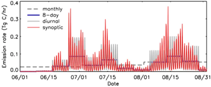
Fig. 1.GFEDv2 time series of total biomass burning emission rates (Tg C/hr) in North America (180◦–60◦W; 30◦–80◦N) for June–
August 2004. GFEDv2 inventories withmonthly,8-day,diurnal, andsynopticvariations are shown.
typically occurs from 13:00 to 18:30 local time and distinctly earlier in heavily forested regions in the tropics and sub-tropics (Giglio, 2007). This diurnal cycle, together with the diurnal variability of atmospheric boundary layer, can con-ceivably influence the transport and deposition of biomass burning emissions. Thus, we were motivated to imple-ment a diurnal cycle to the8-dayGFEDv2 inventory to ac-count for the diurnal variability of forest fires. We used the 8-day GFEDv2 emission inventory as a starting point. We first constructed a mean diurnal cycle with a 3-h time step based on the Automated Biomass Burning Algorithm (ABBA) active fire observations (Prins et al., 1998). The ABBA fire products are available only in the Western Hemi-sphere from the Geostationary Operational Environmental Satellites (GOES). Specifically, for 5 regions (boreal North America, temperate North America, Central America, north-ern South America, and southnorth-ern South America) we con-structed mean diurnal cycles of active fires for the four most abundant land cover classes in the MODIS land cover prod-uct (MOD12C1v4, UMD cover types). The diurnal cycles from the top four land cover classes were weighted by their relative GFEDv2 emissions to obtain a single mean diurnal cycle for the region.
In the Eastern Hemisphere where there is no GOES cover-age, we constructed a mean diurnal cycle using information obtained from the Western Hemisphere. First, we mapped Eastern Hemisphere regions to Western Hemisphere regions based on latitude and land cover. We then used the distribu-tion of MODIS land cover and GFEDv2 emissions in each Eastern Hemisphere region to construct a weighted diurnal cycle from the diurnal cycles for each land cover class in the corresponding Western Hemisphere region. The 3-hourly di-urnal coefficients were multiplied by each day’s emissions (from8-dayGFEDv2) to derive thediurnalGFEDv2 emis-sion inventory.
It is conceivable that forest fires and the resulting emis-sions may be influenced by synoptic weather conditions. For example, high wind speed and less precipitation may en-hance burning hence emissions while large precipitation may suppress forest fires. It is thus essential to account for this
synoptic variability in forest fires. Here we use the Initial Spread Index (ISI, Van Wagner, 1987) for that purpose. ISI indicates the fire favorability of synoptic weather conditions and the expected rate of fire spread. We computed ISI within each GFEDv2 8-day period using GEOS-4 meteorological parameters including temperature, relative humidity, wind speed, and precipitation. These meteorological variables at noon local time were used and re-sampled to 1◦×1◦ grids.
The exception is precipitation, which was aggregated to 24-h totals. The derived ISI was then used to re-distribute emis-sions within each 8-day period. This synoptic variability is then superimposed onto the diurnal inventory. This treat-ment added the day-to-day variation to the diurnal inven-tory, while keeping the diurnal variation within each day un-changed. The resulting inventory is referred to as synoptic GFEDv2 that combines both diurnal and synoptic variations. We would like to point out that the8-dayGFEDv2 inventory (and thediurnalinventory as a result) likely already includes some synoptic variability. That is because the8-day inven-tory was in part constrained by active fire counts, which are presumably influenced by synoptic weather conditions.
A comparison of themonthly,8-day,diurnal, and synop-ticGFEDv2 inventories is shown in Fig. 1 for North America (180◦–60◦W; 30◦–80◦N) during the summer 2004 fire
sea-son. Emissions increased from June to August in themonthly inventory. The higher-temporal resolution inventories, espe-cially thediurnalandsynopticinventories indicate that large emissions were concentrated in short periods. Major fires and associated emissions occur in late June through early July, in mid-July, and throughout much of August. Signif-icant diurnal variations are seen in thediurnalandsynoptic inventories. Thesynopticinventory shows large day-to-day variability. The general features of day-to-day variation in oursynopticinventory are very similar to that in the fire emis-sion inventories derived by Pfister et al. (2005) and Turquety et al. (2007). However, in comparison to these two invento-ries, oursynopticinventory has lower emission rate during late July and higher emission rate during mid-August.
4 Injection heights of biomass burning emissions
the pyro-convection to background meteorology. We exam-ine here the effects of different plume injection height pa-rameterizations on the model simulation of biomass burning long-range transport.
It is conceivable that the pyro-convection at the fire sources shows distinct characteristics compared with the pas-sive convection driven by the meteorology. Fire-produced buoyancy is naturally associated with abundant pollutants such as CO, NOx, and smoke, therefore the potential for sig-nificant atmospheric impact is much greater than for ther-mal convection unrelated to fire (Fromm et al., 2005). How-ever, many previous modeling studies release biomass burn-ing emissions exclusively within the PBL, which does not ex-plicitly treat the fire-induced convection. To represent pyro-convection processes in model simulations, biomass burning emissions can be injected to different vertical layers, emu-lating the effect of fast vertical mixing in the source regions. Recently, some efforts have been made to derive this injec-tion height from the energy of fires and the stability of lo-cal atmosphere through empirilo-cally- (Lavou´e et al., 2000) or physically-based (Freitas et al., 2006, 2007) parameteriza-tions. However, the empirical parameterizations were usu-ally derived from limited observations and may not apply to other smoke plumes. The physically-based methods require accurate measurements of fire energy and local meteorology, which are often not available. Direct observations of for-est fire injection height to validate these injection models are still sparse. Space-based remote sensing instruments are be-ginning to provide measurements of injection heights in fire source regions using stereo imaging (e.g. Kahn et al., 2007; Val Martin et al., 2009), and smoke plume heights downwind from active sensors such as the CALIPSO Lidar (Labonne et al., 2007).
A new stereoscopy-based technique has been recently de-veloped to determine smoke plume injection height from satellite observations (Kahn et al., 2007, 2008; Nelson et al., 2008; Moroney et al., 2002). In this method, smoke plumes were identified using the MODIS thermal anomaly and the multi-angular images from the Multi-angle Imaging SpectroRadiometer (MISR). The wind-corrected height for each smoke pixel was derived using a high-resolution stereo-matching technique, with an uncertainty of about ±500 m (Naud et al., 2005). This new approach represents a refine-ment of that developed for the MISR Standard Stereo Height product (Moroney et al., 2002). Detailed validation of the MISR-derived plume height is still challenging due to limited coverage of MISR measurements and the lack of coincident in situ observations. For some smoke, the fires occur outside the MISR field-of-view, and sometimes for other reasons, it can be difficult to determine the evolution of plume height. In these cases, it is uncertain whether the smoke was injected or advected by regional meteorology to the observed heights. We called such events smoke clouds, and assume the derived heights represent the actual injection heights. Based on this method, plume heights for more than 600 smoke plumes and
Emission rate (g C/m /hr)2
0 0.01 0.02 0.05 0.1 0.2
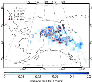
Fig. 2. Spatial distribution of GFEDv2 emissions (g C/m2/hr) in
Alaska and western Canada during June–August 2004 (blue). Also shown are MISR-derived heights of smoke plumes (brown circles) and smoke clouds (grey circles). Data are from Nelson et al. (2008).
smoke clouds over Alaska and the Yukon Territory during the summer of 2004 have been derived (Fig. 2). The average, maximum, and minimum plume heights observed during this period were 0.97 km, 4.5 km, and 0.18 km, respectively. We found between 10% and 30% of smoke plumes reached the free troposphere, even considering the uncertainties in smoke plume height retrieval and PBL height (Kahn et al., 2008).
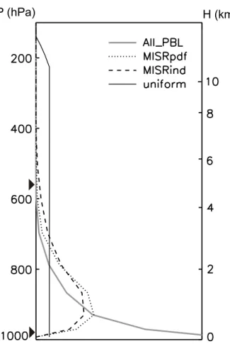
Fig. 3.Vertical profiles for releasing biomass burning emissions in Alaska and western Canada during summer 2004, calculated using All PBL, MISRpdf, MISRind, anduniforminjection height distri-butions as described in Table 1. The two triangles represent the altitudes of maximum and minimum injection heights as observed by MISR in Alaska and western Canada during summer 2004.
individually (hereafter referred to asMISRind). In this ap-proach, when the height of a smoke plume or cloud is more than 2 km above terrain, as observed by MISR, emissions in the model grid box containing the plume are released to the model layer corresponding to the MISR-derived plume height. Since fires usually last for several days, we assume that this high-altitude injection lasts through the 8-day pe-riod. A single PDF profile derived from the rest plumes is used to distribute other fire emissions into model vertical lay-ers. On average, about 10% of the emissions are from those plumes individually treated in the simulation. This approach is based upon the hypothesis that the most intense fires (area and biomass burned, energy release, emissions, etc.) fol-lowed by injection to high altitudes contribute the most to the long-range transport of biomass burning emissions. Since the MISR smoke plume height product we used only includes Alaska and western Canada, we applied the MISR derived
profiles (MISRpdf andMISRind) to these regions only. In other regions, including central Canada where considerable fires were present during the summer 2004, we still use the ALL PBLdistribution. Lastly, we conducted a simulation in which biomass burning emissions were uniformly (in mass mixing ratio) distributed through the tropospheric column up to 200 hPa (hereafter referred to asuniform). This approach is similar to that used in several previous studies (Leung et al., 2007; Turquety et al., 2007; Hyer et al., 2007) although we choose a simpler average configuration. It clearly rep-resents an extreme scenario in which certain percentages of emissions from each boreal forest fire were injected to the middle and upper troposphere. The four vertical profiles for plume injection,All PBL,MISRpdf,MISRind, anduniform are shown in Fig. 3.
5 Model simulations and observations
To examine the effects of the temporal and vertical con-straints on biomass burning emissions, we conducted GEOS-Chem simulations of CO and aerosols in which the GFEDv2 biomass burning emissions inventories described in the pre-vious sections were used. In the CO simulation, we track CO emitted from different source types and regions. This enables the separation of North American forest fire emis-sions of CO from other sources and/or regions. The simula-tions were conducted for January–August 2004 with the first five months as initialization. Our analysis focuses on the last three months, June–August. We archived model output of 3-h average concentrations of tagged CO tracers and aerosols.
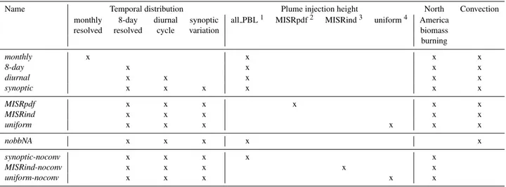
Table 1.GEOS-Chem simulations with different GFEDv2 biomass burning emission inventories (different temporal distributions and plume injection heights) and with or without convection.
Name Temporal distribution Plume injection height North Convection
monthly 8-day diurnal synoptic all PBL1 MISRpdf2 MISRind3 uniform4 America
resolved resolved cycle variation biomass
burning
monthly x x x x
8-day x x x x
diurnal x x x x x
synoptic x x x x x x
MISRpdf x x x x x x
MISRind x x x x x
uniform x x x x x x
nobbNA x x x x x
synoptic-noconv x x x x x
MISRind-noconv x x x x x
uniform-noconv x x x x x
1all PBL: uniformly released throughout the PBL.
2MISRpdf: vertically dirstributed according to a probability distribution function (PDF) of MISR-derived plume heights. 3MISRind: similar to MISRpdf, but with high smoke plumes treated indivicually.
4uniform: uniformly released throughout the tropospheric column up to 200 hPA.
To evaluate the model performance, we compared model results with aircraft, satellite, and ground-based observations of CO and aerosols. The INtercontinental chemical Trans-port EXperiment – North America (INTEX-NA) (Singh et al., 2006) was conducted over the continental United States and western North Atlantic during the summer of 2004. A focus of this experiment was to quantify and character-ize the inflow and outflow of aerosols and trace gases over North America. We used the 5-min aggregated CO mix-ing ratio and aerosol absorption data from INTEX-NA, for which the NASA DC-8 was the principle platform. The mea-sured 530 nm absorption coefficient (babs, m−1) from Parti-cle Soot Absorption Photometers was used to derive the BC mass concentration (M, g/m3) as follows: M=babs
Eabs, where
Eabs=10 m2g−1 is the assumed BC mass absorption effi-ciency (Horvath, 1993; Andreae and Gelencs´er, 2006). Ver-tical profiles of CO mixing ratio and BC mass concentration were derived from the DC-8 measurements and compared with GEOS-Chem results.
The Measurement of Pollution in the Troposphere (MO-PITT) instrument aboard the Earth Observing System (EOS) Terra satellite measures upwelling infrared radiation and has been retrieving CO mixing ratios and total column amounts since 2000 (Drummond et al., 1996; Deeter et al., 2003). CO mixing ratios are reported for six pressure levels: 850, 700, 500, 350, 250, 150 hPa, and at the surface, for global clear-sky measurements. The retrieved CO profile is a linear combination of the true profile and a fixed a priori profile.
MOPITT also retrieves CO column, which is the integral of the CO mixing ratio at each level, using an averaging kernel that is most sensitive to the middle troposphere (Deeter et al., 2003). MOPITT views the Earth with a 22 km×22 km spatial resolution and covers the entire globe every 3 days. In this study, we compare spatial distribution and time series of CO column over North America from the model simula-tions with the MOPITT V3 Level 3 (MOP03, gridded daily averages) CO retrievals. Only the daytime (10:45 local time) MOPITT CO columns were used in our comparison because the nighttime measurements have not been validated (Heald et al., 2004).
NASA’s AErosol RObotic NETwork (AERONET, Holben et al., 1998) provides globally distributed near real time ob-servations of aerosol spectral optical depths at wavelengths of 340, 380, 440, 500, 670, 870, 940 and 1020 nm (Holben et al., 1998). During the summer of 2004, there were more than 80 automatic Sun-sky spectral radiometer sites operat-ing. In this study we compared model simulated aerosol re-sults against AERONET Level 2.0 cloud-screened, quality-assured 500 nm AOD data (Smirnov et al., 2000).
We used CO from MOPITT and aircraft measurements to compare with our simulation because these measurements provided CO information in the middle and upper tropo-sphere, where the long-range transport has largest effect. Measurements of surface CO are also available, but the vari-ability of surface CO is often dominated by other factors such as fossil fuel emissions. Therefore it is difficult to use these measurements to assess the importance of temporal variabil-ity and injection height of biomass burning. In addition to aerosol measurements from IMPROVE and AERONET, we also compared model results with AOD products from satel-lite remote sensing instruments (e.g. MODIS and MISR). Initial results showed that the differences between differ-ent model simulations are much smaller than the model-observation difference and MODIS-MISR difference. Thus we will not present these comparisons in this study.
6 Results
6.1 Simulated CO and BC in response to biomass burning emission temporal and vertical distribution The primary goal of this study is to assess the impact of vari-ous temporal and vertical emission distributions on the trans-port and mixing of North American biomass burning CO and aerosols. In this section, we compare the CO and BC re-sults from different GEOS-Chem simulations as summarized in Table 1. The differences among the model simulations can then be attributed to different temporal and/or vertical distributions of biomass burning emissions. We present the comparisons of CO mixing ratios in different model layers in 6.1.1. In 6.1.2, we show how the temporal distributions and injection heights of biomass burning emissions affect CO and BC total column burdens in North America.
6.2 CO mixing ratios
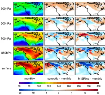
Modeled CO mixing ratios at five pressure levels (surface, 850 hPa, 700 hPa, 500 hPa, 300 hPa) over North America and adjacent oceans from themonthly simulation are shown in the left column of Fig. 4. The values are averages for June– August 2004. In addition to the anthropogenic emissions over the Midwest and East Coast, emissions from boreal for-est fires in Alaska and wfor-estern Canada and their subsequent long-range transport lead to widespread enhancement in CO throughout the lower to middle troposphere.
Fig. 4. Model simulated 3-month (June–August 2004) average
CO mixing ratios (ppbv) at five pressure layers (surface, 850 hPa, 700 hPa, 500 hPa, 300 hPa) from themonthlysimulation, and the differences due to the adding of temporal constraints (synoptic– monthly), and due to the adding of both temporal constraints and MISRindinjection height of biomass burning emissions (MISRind –monthly).
In comparison with themonthlysimulation, effects of ad-ditional temporal and vertical constraints are clearly seen in the middle (synoptic – monthly) and right (MISRind – monthly) columns of Fig. 4. The difference between the syn-opticandmonthlysimulations (middle column, Fig. 4) repre-sents the cumulative effect of all three temporal constraints, i.e. the 8-day redistribution, the diurnal cycle, and the syn-optic day-to-day variation. Relative to themonthly simula-tion, thesynopticsimulation decreases CO levels throughout the tropospheric column over the biomass burning source gions, and increases CO levels downwind of the source re-gions. The largest increase occurs at 300 hPa over much of North America.
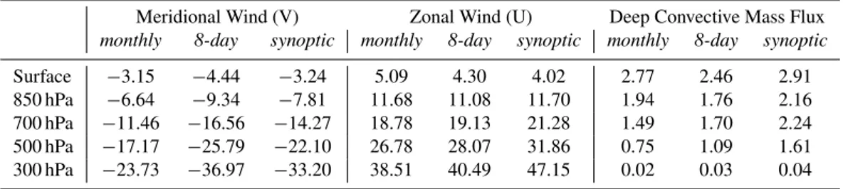
Table 2. Biomass burning emission-weighted mean meridional (V) winds (m/s), zonal (U) winds (m/s), and deep convective mass fluxes (10−2Pa/s) over Alaska and western Canada during summer 2004. Positive values indicate eastward, northward and upward winds and fluxes.
Meridional Wind (V) Zonal Wind (U) Deep Convective Mass Flux monthly 8-day synoptic monthly 8-day synoptic monthly 8-day synoptic
Surface −3.15 −4.44 −3.24 5.09 4.30 4.02 2.77 2.46 2.91
850 hPa −6.64 −9.34 −7.81 11.68 11.08 11.70 1.94 1.76 2.16
700 hPa −11.46 −16.56 −14.27 18.78 19.13 21.28 1.49 1.70 2.24
500 hPa −17.17 −25.79 −22.10 26.78 28.07 31.86 0.75 1.09 1.61
300 hPa −23.73 −36.97 −33.20 38.51 40.49 47.15 0.02 0.03 0.04
Fig. 5. Differences of model simulated 3-month (June–
August 2004) average CO mixing ratios (ppbv) at five pressure lay-ers (surface, 850 hPa, 700 hPa, 500 hPa, 300 hPa) due to the adding of each temporal constraint on biomass burning emissions.
wind speeds are also higher in thesynopticsimulation (see Table 2), indicating stronger horizontal advection of CO.
Going from monthly to synoptic GFEDv2 not only en-hances transport, but also changes the transport direction. For example, negative values over the sub-Arctic regions in Fig. 4 indicate that the northward transport is decreased in thesynopticsimulation. On the other hand, increased influ-ence of biomass burning CO is seen at mid-latitude North America in thesynopticsimulation. This is consistent with the much stronger, southward (negative values), emission-weighted meridional winds in thesynopticsimulation at all pressure levels (Table 2).
Also shown in Fig. 4 (right column) are the changes in CO mixing ratios relative to themonthly simulation when both the temporal constraints and MISR-derived injection heights were used (MISRind – monthly). The spatial patterns out-side of fire source regions are similar to those ofsynoptic –
monthly(Fig. 4, middle column), indicating that the overall effect of plume vertical injection as implemented inMISRind is smaller than that of the temporal distributions. However, in the source regions, the use ofMISRindvertical distribu-tion significantly increases the CO mixing ratios at 700 hPa while decreases CO at the surface. The enhancement of CO at 700 hPa over eastern North America is also stronger than that ofsynoptic – monthly.
Figure 5 shows the relative importance of each tempo-ral constraint. A mean diurnal cycle as implemented in the model has a relatively minor effect on the export and long-range transport of biomass burning CO. It somewhat de-creases the surface CO level while increasing CO mixing ratios at high altitudes (Fig. 5, middle column). Matichuk et al. (2007) studied the effect of a diurnal cycle on biomass burning aerosols in southern Africa and reached similar con-clusions.
Relative to the inclusion of a diurnal cycle, going from monthly to8-day GFEDv2 inventory (Fig. 5, left column) and the inclusion of a synoptic constraint (Fig. 5, right col-umn) lead to larger changes in simulated CO distribution. Compared to the monthly simulation, the use of the8-day GFEDv2 enhances the southward transport and therefore in-creases the CO mixing ratios in southern Canada and north-ern US. This change can also be linked to the increased coin-cidence of fire emissions and southward winds (see Table 2). With the use of the synoptic constraint, the enhancement of southward transport is decreased. More transport is toward the high latitudes over northeastern Canada.
Fig. 6. Differences of model simulated 3-month (June– August 2004) average CO mixing ratios (ppbv) at five pressure lay-ers (surface, 850 hPa, 700 hPa, 500 hPa, 300 hPa) due to the use of each injection height distribution of biomass burning emissions.
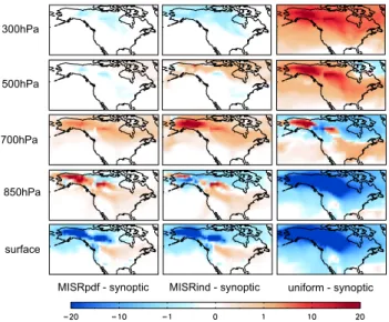
theMISRpdf andAll PBLdistributions (Fig. 3). Since most high smoke plumes individually treated in theMISRind dis-tribution reside between 600 hPa and 800 hPa, theMISRind simulation also shows large increase of CO at 700 hPa. The increase of CO is also seen up to the 500 hPa level over high latitudes. By injecting much more emissions into higher altitudes (Fig. 3), theuniform distribution significantly de-creases the CO mixing ratios in the lower troposphere and increases CO in the upper troposphere. The affected region covers a much larger area than that from theMISRpdf or MISRindsimulations.
We also calculated the BC concentration changes due to the use of different biomass burning emission temporal dis-tributions and injection height disdis-tributions (not shown here). Overall the effects are similar to that for CO mixing ratios shown in Figs. 4–6. A noticeable difference is that the ef-fects on BC at high altitudes are much smaller than for CO. In addition, the domain in which injection height reduces the surface BC concentration is smaller than that for CO. 6.3 Column burdens
In this section, we investigate the sensitivity of CO and BC column burdens to different biomass burning emission tem-poral distributions and injection height profiles. Figure 7 shows the changes of 3-month (June–August 2004) average CO and BC column burdens after using the temporal con-straints, the MISR-derived injection height distributions, and both. Since the relative differences of CO and BC column burdens between theMISRpdf andMISRindsimulations are small, hereafter we only concentrate on theMISRind simula-tion.
40N 60N
120W 80W 160W
80N
40N 60N
120W 80W 160W
80N
40N 60N
120W 80W 160W
80N
40N 60N 80N
120W 80W 160W
40N 60N 80N
120W 80W 160W
40N 60N 80N
120W 80W 160W
Fig. 7.Impacts of biomass burning emission temporal and injection
height distribution on simulated 3-month (June–August 2004) aver-age CO (left columns) and BC (right columns) column burdens in North America. The absolute differences (kg/km2) are shown in red and blue grid cells. The relative changes (in percentage) are shown in line contours.
With biomass burning emission temporal constraints added, more emissions are distributed during shorter inter-vals. Previous discussions on Fig. 4 and Table 2 show that emissions during these shorter intervals are subject to stronger convection and southward transport. Therefore, the CO and BC column burdens are reduced in the source re-gions and increased in the downwind rere-gions, particularly south of 60◦N, as evident in the difference between the
syn-opticandmonthlysimulations (Fig. 7a). TheMISRind sim-ulation includes all the temporal constraints (8-day, diurnal, and synoptic) therefore the difference between theMISRind andsynopticsimulations is attributed to the effect of plume injection (see Sect. 4). Lifetimes of pollutants including CO and BC are typically longer in the free troposphere. Thus the overall effect of applying theMISRind vertical distribution is decreasing the CO and BC burdens in the biomass burn-ing source regions and increasburn-ing them downwind, as shown in the difference between theMISRindandsynoptic simula-tions (Fig. 7b). The combined effect of including both the temporal constraints and MISR-derived emissions injection height distributions, as the difference between theMISRind andmonthlysimulations shows, is mainly determined by the temporal constraints (Fig. 7c).
Fig. 8. Time series of enhanced total CO and BC burdens (Tg) in North America (180 W–60 W, 30 N–80 N) for June–August 2004. The enhancement is the difference between simulated CO/BC bur-den and that from thenobbNAsimulation. The 3-month mean val-ues for the enhancement from each simulation are shown in the leg-end.
considerably different. Relative to CO, BC burden decreases in a smaller region near the biomass burning sources, as ex-pected, considering the shorter lifetime of BC. Over eastern North America, the use of temporal constraints and MIS-Rind injection height increases BC burden as much as 20%, whereas the largest change in CO burden is only about 2% (Fig. 7c).
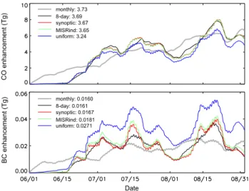
Figure 8 shows GEOS-Chem simulated time series of CO and BC burden enhancements within the North American domain, defined as 180◦–60◦W, 30◦–80◦N, during June–
August 2004. The enhancements were calculated as the difference between thenobbNA simulation in which North American biomass burning (mostly in Alaska and western Canada) were turned off, and other simulations (see Table 1). The larger slopes in Fig. 8 correspond to intensive emis-sions shown in Fig. 1. Overall, the use of emisemis-sions with higher temporal resolutions shows more temporal variability, and generally increases the enhancements during periods of extensive fire occurrences such as later June, mid-July, and mid-August. However, there is no significant change in the three-month mean values (shown in the legend of Fig. 8) of enhancements for CO and BC from simulations with differ-ent temporal distributions of emissions. We also notice that in the monthlyand 8-daysimulations in which the diurnal variability of biomass emissions is not represented, a diurnal cycle of total burden is clearly seen for BC, but not for CO. This diurnal signal of the BC burden, not to be confused with that from diurnal cycle of fires, may originate from the diur-nal patterns of aerosol removal processes (Nicholson, 1988). Figure 8 also demonstrates the difference between the in-jection height effects on BC and CO. The MISRind and
uniform simulations, especially the latter, show large in-creases of total BC burdens due to longer lifetimes of BC once injected into the free troposphere. Therefore, the to-tal BC enhancement is larger when some fire emissions are above the PBL (MISRindanduniform). The consequence for the CO burden, however, is the opposite. The amount of in-creased CO transported out of the North American domain is so large that increased transport removal outweighs the in-crease of CO burden within the domain due to the longer lifetime.
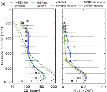
6.4 Comparison of modeled CO and BC vertical profiles with INTEX-NA observations
The role of biomass burning injection height distribution in affecting the simulated vertical profiles of trace gases and aerosols is discussed in this section. We compared our model results with DC-8 aircraft measurements during the INTEX-NA experiment over eastern North America (Fig. 9). We compared CO and BC vertical profiles averaged for the en-tire INTEX-NA period and from specific flights. In the lat-ter case, the selected flights correspond to days with appar-ent influence of forest fires in Alaska and western Canada. GEOS-Chem results are sampled along the flight tracks at the time of measurements (see http://www.espo.nasa.gov/ intex-na/flight reps.html).
Overall, GEOS-Chem captures the main features of the mean and individual CO profiles (Fig. 9a, b), even with biomass burning emissions distributed within the PBL only (in thesynopticsimulation). The largest bias occurs in the low troposphere, where the model overestimates the CO mix-ing ratios. This may be due to several factors includmix-ing emis-sion estimates that are too high, or by model biases such as OH levels that are too low, or convection that is too weak. Detailed exploration of this discrepancy is beyond the scope of this paper. Due to the different temporal and spatial scales between model results and the INTEX-NA measurements, GEOS-Chem is not expected to capture some extreme events of high CO. Therefore, there are occasional large differences between model results and the mean values of observations (e.g. at 350 hPa on 18 July).
o
Fig. 9a. Comparisons of vertical CO and BC profiles from model
simulations and from measurements during the 2004 INTEX-NA experiment for all flights. Grey points and bars are mean values and standard deviation of the observations at each level. Black squares are median values of the observations at each level. All model re-sults are sampled along the flight trajectories.
07/15 07/18 07/22 08/02 08/13
07/15 07/18 07/22 08/02 08/13
Fig. 9b.Same to Fig. 9a, but for representative individual flights.
synopticCO profiles), the differences between thesynoptic andMISRindprofiles are almost negligible. It is not obvious from Fig. 9 that theuniformsimulation improves the agree-ment with the aircraft observations in the upper troposphere, either in the average sense (left panel, Fig. 9a) or during in-dividual flights (top row, Fig. 9b). It does show an enhanced plume in the upper troposphere during the flight on 15 July but significantly overestimates CO by more than 20 ppbv dur-ing the flight on 13 August.
The shape of CO profiles is determined by moist convec-tion to a large degree. By turning off convecconvec-tion, GEOS-Chem significantly underestimates CO at high altitudes and overestimates CO at low altitudes. The model sensitivity to biomass burning injection height is also affected by con-vection. Most flights during INTEX-NA were thousands of kilometers away from the fire sources in Alaska and west-ern Canada. During long-range transport, vertical mixing processes including convection carry more pollutants out of the PBL, thereby reducing the effect of biomass burning injection height. Figure 9 shows the difference between simulations with different injection height distributions is smaller when convection is turned on.
The vertical profile of BC is an important factor in de-termining BC radiative effect (Haywood and Ramaswamy, 1998; Penner et al., 2003). However, it is extremely diffi-cult to compare the modeled BC vertical profile with mea-surements for several reasons. First, the data in each layer are more variable than for CO (shown with grey error bars in Fig. 9). Second, the assumed value of mass absorption efficiency, which is used to convert measured absorption ex-tinction to BC concentration, may vary by more than a factor of two (Fuller et al., 1999; Andreae and Gelencs´er, 2006). Third, the uncertainty caused by the deposition scheme used in the model may have a large impact on the comparison. De-spite these uncertainties, the comparison (Fig. 9) shows small concentration differences between thesynopticandMISRind simulations.
6.5 Comparison of modeled CO total column with MOPITT observations
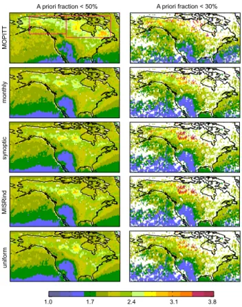
The MOPITT CO retrieval is most sensitive to the middle troposphere (Deeter et al., 2003). For direct comparison with MOPITT CO columns, GOES-Chem simulated CO profiles were sampled along MOPITT orbital tracks and then inter-polated to the six standard MOPITT pressure levels and the surface. The resulting model profiles were then convolved with MOPITT averaging kernels and a priori profile (Em-mons et al., 2004). To minimize the a priori influence and compare model results against actual measured information, we used MOPITT retrievals with a priori contributions less than a preset threshold. Two thresholds (50% and 30%) were used to show the sensitivity of the comparison to this value, as discussed below.
Fig. 10.Comparison of 3-month (June–August 2004) average CO column (1018molec/cm2) from GEOS-Chem simulations and from MOPITT retrievals. MOPITT averaging kernel and the a priori CO profile were applied to model results. Two a priori critical fractions (50% and 30%) were used to filter out samples with large a priori contributions.
downwind region, where the correlation coefficient increases from 0.61 for themonthlyto 0.69 for thesynoptic. The use of MISRindanduniforminjection height distributions decreases the CO column in the source regions, but they cause little change downwind. Over eastern Canada, the large discrep-ancy still exists when the temporal constraints are applied. Previous modeling studies have shown similar large model versus MOPITT CO column discrepancies and point to poor treatments of biomass burning emissions as a primary rea-son (Bian et al., 2007; Turquety et al., 2007). Our results show that even with a large portion of the fire emissions dis-tributed in the middle and upper troposphere, as in the uni-formsimulation, the model still underestimates CO columns over this region. Therefore, the lack of fire emission injection above the PBL is unlikely to be the only or main cause of the large discrepancy. We should also bear in mind that the MO-PITT measurement itself has uncertainty and bias. Emmons et al. (2004) showed that the MOPITT retrievals have an un-certainty of 20–40% at 500 hPa, and a bias of−0.2%–8% compared to in situ CO measurements from aircraft.
Figure 10 also shows that the comparison is sensitive to the value of a priori critical fraction. The comparisons between
model and MOPITT CO columns over the fire source regions are better when a priori critical fraction of 30% is used (cor-relation coefficientR=0.54), compared with 50% (R=0.46). Downwind, particularly over northeastern North America, fewer data samples satisfy the criterion of a priori fraction be less than 30%, which makes the comparison more diffi-cult. Our simulated CO column distribution (with a priori fraction<50%) is similar to that in Turquety et al. (2007), in which the same GEOS-Chem model with a different biomass burning emission inventory was used.
We further compare our model results with MOPITT re-trievals by showing the time series of mean CO columns over a source domain (150◦–110◦W, 55◦–70◦N) and a downwind
domain (110◦–60◦W, 50◦–70◦N) (Fig. 11). The domains are
indicated in Fig. 10. Since MOPITT provides global cover-age every 3 days, we used the 3-day avercover-age CO. Again, we applied two a priori critical fractions (50% and 30%).
The phase of temporal variability agrees well between MOPITT and all the GEOS-Chem simulations in the biomass burning source regions except the monthly. The correla-tion coefficient is considerably smaller in themonthly case (R=0.08) than the other cases (R>0.60). In general, the agreement is better in the source domain than in the down-wind domain. Differences in magnitude between measure-ments and simulations are present, particularly during peri-ods of major fire occurrences (represented by high emissions as shown in Fig. 11). For example, all model simulations underestimate CO columns in mid-July in the downwind domain, and overestimate CO in mid-August in both the source and downwind domains. This suggests that using MODIS fire counts to re-distribute biomass burning emis-sions may miss some important fire events (e.g. clouds may mask fire hot spots) and incorrectly represent the day-to-day variation.
The use of MISRind injection height distribution causes only small changes in the results. Theuniform simulation produces smaller CO column in the source domain than the synoptic simulation, which sometimes shows better agree-ment with MOPITT but sometimes shows larger bias. The a priori critical fraction has a larger effect on the simulated CO column than on the MOPITT retrievals. Overall, the bias be-tween model simulations and measurements is higher when we use a smaller critical fraction, partly due to the smaller number of data samples after applying the 30% restriction.
6.6 Comparison of modeled results with surface aerosol and total AOD measurements
Fig. 11.Time series of mean CO column (1018molec/cm2) in a source domain (150◦–110◦W, 55◦–70◦N) and a downwind domain (110◦–
60◦W, 50◦–70◦N) from MOPITT retrievals and GEOS-Chem simulations. Each point represents a value of three-day average CO column. Locations of these domains are shown in Fig. 10. MOPITT averaging kernel and the a priori CO profile were applied to model results. The correlation coefficients between MOPITT and model simulations are shown in the legend. Two a priori thresholds (50% and 30%) were used to filter out samples with large a priori contributions. Grey bars represent total biomass burning emissions (Tg C/3-day) in the domains.
are not shown, as they are very similar to the8-dayand MIS-Rindsimulations, respectively. Among the four IMPROVE sites, DENA1 (63.7◦N, 149.0◦W) is very close to major fires. AMBL1 (67.1◦N, 157.9◦W) is a Northern Alaskan site
with no major fires, but is not far away from the major fire sources in Alaska and western Canada. MELA1 (48.5◦N,
104.5◦W) and BOWA1 (47.9◦N, 91.5◦W) are near the
US-Canada border and are frequently affected by smoke from boreal fires in Alaska and western Canada.
We find the day-to-day variability in the model simulations resembles that from the IMPROVE measurements, except for themonthlysimulation. This again indicates the importance of using emissions with at least an 8-day temporal resolu-tion. Thesynopticsimulation, which includes both the di-urnal cycle and the synoptic variability of biomass burning emissions, shows more temporal variability. But its effect on the comparison with measurements is smaller than switch-ing from the monthly to the 8-day emissions. The use of
MISRind injection height distribution improves the simula-tion in the source region (DENA1 site) compared with no vertical injections, particularly during mid-July and late Au-gust. For the downwind sites, the BC surface concentrations from theMISRindsimulation are similar to those from the synoptic simulation. Theuniform simulation shows better agreement with IMPROVE measurements at the downwind sites. However, in the source region (DENA1 site), the uni-form simulation often significantly underestimates surface BC. Therefore, high-elevation injection of biomass burning smoke injection might be episodic and possibly related to in-dividual high-energy fire events and suitable meteorological conditions, or even high-energy fires might tend to inject a large fraction of smoke into the PBL than theuniform simu-lation assumes.
Fig. 12. Time series of surface BC concentrations (µg/m3) from model simulations and IMPROVE observations (filled square boxes). IMPROVE measurements are 24 h average values which were recorded each 3 days. Upper panel for each site shows the sensitivity to temporal constraints. Bottom panel for each site shows the sensitivity to injection height.
Fig. 13. Time series of 500 nm AOD from model simulations and AERONET observations. Daily mean values and uncertainty ranges of
sites (Barrow; 71.3◦N, 156.6◦W; Bratts Lake; 50.3◦N,
104.6◦W; Resolute Bay; 74.7◦N, 94.9◦W). We calculated
total AODs from GEOS-Chem simulated aerosol concen-trations and pre-assumed microphysical and optical proper-ties associated with all aerosol species (Park et al., 2003). The use of 8-day temporal resolution and synoptic constraint improves the timing of high-AOD occurrences over both the source and downwind regions. For example, the corre-lation coefficients between observations and model results increased from 0.36 to 0.66 at Bonanza Creek and from 0.21 to 0.74 at Barrow. But there are still large discrepan-cies between simulated and AERONET AODs, particularly during high-AOD events. ThenobbNAsimulation produces very small AODs during these events, indicating a domi-nating contribution from North American biomass burning emissions. A comparison with satellite observed AODs from MISR and MODIS (not shown here) also shows the under-estimation of GEOS-Chem model results. The low bias in the simulated AOD over biomass burning regions has been reported by several previous studies (Matichuk et al., 2007; Pfister et al., 2008). Pronounced spatiotemporal variability of AOD and different sampling between the measurements and the model may partly explain the discrepancy. The dif-ferent assumptions of aerosol properties used in the satellite retrievals and model calculations may play a role as well. Recent studies of simulating directly satellite observed ra-diances in CTMs to retrieve AOD show better agreement between GEOS-Chem and MODIS (Drury et al., 2008). It avoids the aforementioned inconsistency. Figure 13 also shows the use of theMISRpdf anduniforminjection height distributions only has minor change in the simulated AOD.
7 Discussion
Conflicting results have been reported in past work on the effect of fire-induced lifting in model simulations. Some comparisons between models and measurements (e.g. Leung et al., 2007; Freitas et al., 2006) show the best agreement when a large portion of fire emissions are injected into the middle troposphere. Turquety et al. (2007) concluded that a significant fraction of emissions from the largest fires should be injected into the upper troposphere in order to match MO-PITT observations. Lamarque et al. (2003) and Colarco et al. (2004), however, showed that releasing of fire emissions at the surface may produce results similar to releasing emis-sions at high altitude, because in these models, local convec-tion immediately lifts the polluconvec-tion into the free troposphere. Our results show that averaged over the 2004 summer fire season, the overall effect of using the MISR-derived injection height distribution is small. The change of simulated CO col-umn by usingMISRinddistribution is smaller than 1% over most North America (Fig. 7). Compared to CO, the effect of injection height distribution on BC is larger, with 5%–10% increase in total column averaged over summer 2004 after
MISRinddistribution being used. Both CO and BC changes due to the use ofMISRinddistribution are smaller than that caused by applying temporal constraints on biomass burn-ing emissions. The combined effect of usburn-ing the synoptic GFEDv2 and MISRind distribution can increase the mean BC burden over northeastern North America by 10%–20% (Fig. 7).
Previous studies (e.g. Turquety et al., 2007) have shown the use of higher injection heights may enhance the long-range transport of CO and reduce the bias between CO column derived from model simulation and MOPITT re-trievals. Results from this study show that unlike the tem-poral constraints, which reduce the bias between modeled CO and MOPITT CO (Fig. 10), the injection height has lit-tle effect on the comparison. We believe that the lack of biomass burning injection heights above the PBL is unlikely the primary reason for the CO column underestimation over Quebec during 2004 summer. Other adjustments, such as improvements to total biomass burning emission amount, a better representation of emission temporal variability, and a more realistic meteorological field, may be more important.
On a shorter time scale, the injection height may have larger effects. Satellite-derived injection height distribution (MISRind) improves the agreement with surface measure-ments at or near the fire source (Fig. 12). But its effect on AOD is not significant (Fig. 13). We also notice the injection height effect is much smaller in the downwind region. The time series of CO column (Fig. 11), surface BC concentra-tion (Fig. 12), and AOD (Fig. 13), and the vertical profiles of CO and BC (Fig. 9) over northeastern North America show very small difference between thesynopticandMISRind sim-ulations. Even during large fire events, there is no conclusive evidence that the use of biomass burning emissions above the PBL will improve the simulation in the downwind region.
In Fig. 14, we take a fire event as an example to illustrate how the injection height effect is entangled with other uncer-tainties, particularly the meteorology driven transport. This fire event took place in mid-July 2004. High CO concentra-tions at 300 hPa were observed by the DC-8 aircraft during the INTEX-NA experiment on 18 July. We calculated back-ward air trajectories ending in Quebec (centered at 67◦W,
55◦N) at 19 July (00:00 UTC) using the HYbrid
A B A B A B A B
Fig. 14.Simulated daily mean CObbNA (CO from North American biomass burning source) during 13–19 July 2004.(a)CobbNA (ppbv) at
300 hPa from thesynopticsimulation. White line A–B is derived from the back trajectory analysis using the HYSPLIT model. The starting point B [55◦N, 67◦W] is located at 5 km above the ground level and the back trajectory starting time is 00:00 UTC, 19 July . (b)Total
biomass burning emission rate (Tg C/month) in grid cells along the trajectory A–B.(c)CObbNA vertical profile along the trajectory A–B from thesynopticsimulation. Line contours represent the deep convection mass flux (kg/m2/s) from the GEOS-4 reanalysis database. The contour levels are 0.005, 0.01, 0.02, 0.04, 0.06, 0.1 from light dashed line to thick solid line. (d)CObbNA difference along the trajectory A–B between theMISRindandsynopticsimulations. (e)CObbNA difference along the trajectory A–B between theuniformandsynoptic simulations.
height distribution) are shown in Fig. 14a and c. We also plot a contour of deep convective flux from the GEOS-4 me-teorology over CO mixing ratio profiles in Fig. 14c. The hor-izontal and vertical patterns show the rise of fire emissions and the transport of CO from the source region near A to the downwind region near B. This rise and transport are closely related to meteorological conditions. During 13–15 July, de-spite large emissions in the source region, CO concentration in the upper troposphere is small. Strong deep convection from 16 July causes rapid mixing between the near-surface atmosphere and the upper troposphere. CO in the upper tro-posphere is then enhanced and transported to the downwind region. The differences of CObbNA profiles between the MISRind and synoptic simulations are shown in Fig. 14d. Since more emission is assigned to the middle troposphere in theMISRind distribution (see Fig. 3), an increase of CO between 400–600 hPa and a decrease of CO in the PBL can be seen in Fig. 14d. During 13–15 July, when the convec-tion is weak, this signal of injecconvec-tion height distribuconvec-tion is moved to the near downwind region (near the middle of A
and B) without much abatement. However, this signal dis-sipates quickly after 16 July, likely due to the occurrence of strong convections near the fire sources.
Finally let us take a look at a special injection height dis-tribution used in this study. The uniform distribution put more than 50% of the biomass burning emissions into the middle and upper troposphere. It appears that the injection height effect in this simulation can survive the strong verti-cal mixing and cause a significant enhancement downwind (Fig. 14). We find this uniform distribution may produce better results in the downwind region when compared with measurements during some fire events (e.g. CO mixing ratio at middle and high altitudes on 07/18 as shown in Fig. 9b, Surface BC concentration at MELA1 on 08/18 as shown in Fig. 12c). However, we note this injection height distribution is highly unrealistic. It simply assumes all biomass burn-ing emissions follow the same distribution, neglectburn-ing the fact that high injection heights occur only at sporadic fire events when sufficient thermal buoyancy and appropriate at-mospheric stability are available. As shown in previous sec-tions, the use of theuniforminjection height distribution may cause distorted vertical CO and BC profiles (e.g. on 08/13 as shown in Fig. 9b), and too low surface concentrations near the source (at DENA1 and AMBL1 as shown in Fig. 12), at least in some situations. The presence of some cases where theuniformsimulation agrees better with the measurements than theMISRind simulation indicates that MISR observa-tions may miss some high smoke injection events. This can be due to the limited spatial and temporal coverage of MISR radiance measurements, or the blocking of fire hot spots by clouds.
8 Summary
Aerosols and trace gases from boreal forest fires in Alaska and western Canada can be transported to eastern North America, the North Atlantic, and Europe, causing a degrada-tion of air quality and influencing solar radiadegrada-tion and climate. Accurate estimation of this effect needs temporally and spa-tially resolved biomass burning emissions. We simulated CO and aerosols over North America during the 2004 fire season using the GEOS-Chem chemical transport model. We ap-plied different temporal and injection height distributions to the biomass burning emissions, and evaluated model perfor-mance with these constraints by comparing the results with atmospheric measurements from multiple sources.
We find the use of finer temporal resolution biomass emis-sions usually decreases CO and BC near the fire source re-gion, and often enhances long-range transport. Among the individual temporal constraints, switching frommonthlyto 8-dayGFEDv2 and including synoptic variability significantly affect CO and BC distributions. Themonthly-to-8-day con-version often produces more southward transport. The inclu-sion of synoptic constraints is associated with stronger con-vection and more northward transport. Whether this shift of transport is a general phenomenon or is specific to this par-ticular model environment for summer 2004 needs further
investigation. The effect due to the diurnal cycle of biomass burning emissions is minimal.
Averaged over three months during summer 2004, the change of CO and BC due to the use of different injection height distributions is smaller than that due to the use of dif-ferent temporal distributions. The model results are more sensitive to the biomass burning injection height near the source region. Allowing emissions above the PBL lowers surface concentrations and column burdens of pollutants near the source, whereas it increases pollutant concentrations at high altitude and downwind. But overall, the use of MISR-derived injection height distribution increases CO burden in the downwind region only by less than 1%. This is roughly consistent with Pfister et al. (2005), who showed that the CO fire emissions derived from inverse calculations are not sen-sitive to the vertical distribution of emissions.
The BC simulation is more sensitive to the temporal and injection height distributions of biomass burning emissions. The use of these constraints may increase the BC column in eastern North America by 10%–20%. Over the whole US domain, the use of smoke injections above the PBL decreases the total CO burden but increases the BC burden. The shorter lifetime and smaller background concentration for BC are likely reasons for the contrasts between CO and BC.
We compared our model results with CO and BC vertical profiles from INTEX-NA, the CO total column from MO-PITT, surface BC concentrations from IMPROVE, and total-column AOD from AERONET. These comparisons confirm the improvement when satellite data are used to constrain the intra-month variability. In particular, the use of8-day GFEDv2 inventory shows much better agreement with most measurements than the monthly mean emissions.
In comparison to CO from MOPITT and BC from IM-PROVE measurements, the use of MISR-derived injection height profile (MISRind) improves the simulation near the fire sources. The injection height effect is less apparent in the downwind regions. Modeled CO and BC vertical pro-files closely match the INTEX-NA measurements over east-ern North America, even when all the biomass burning emis-sions are distributed within the PBL. The discrepancies be-tween model simulated and MOPITT retrieved CO over Que-bec of Canada can not be simply attributed simply to the lack of biomass burning injections above the PBL. Neither the MISRindnor theuniformprofile significantly reduces the dis-agreement. Reducing uncertainties from other sources, such as a better estimate of total burned area, a more realistic rep-resentation of emission temporal variability, or an improve-ment in moist convection parameterization, may do more to improve model performance.