Atmospheric transport and deposition of Indonesian volcanic emissions

(1)

ACPD

5, 11861–11897, 2005

Indonesian volcanic emissions

M. A. Pfeffer et al.

Title Page

Abstract Introduction

Conclusions References

Tables Figures

◭ ◮

Back Close

Full Screen / Esc

Print Version

Interactive Discussion

EGU

Atmos. Chem. Phys. Discuss., 5, 11861–11897, 2005 www.atmos-chem-phys.org/acpd/5/11861/

SRef-ID: 1680-7375/acpd/2005-5-11861 European Geosciences Union

Atmospheric Chemistry and Physics Discussions

Atmospheric transport and deposition of

Indonesian volcanic emissions

M. A. Pfeffer1, B. Langmann1, and H.-F. Graf2

1

Department of the Atmosphere in the Earth System, Max-Planck-Institute for Meteorology, Hamburg, Germany

2

Department of Geography, University of Cambridge, Cambridge, UK

Received: 6 September 2005 – Accepted: 8 October 2005 – Published: 21 November 2005 Correspondence to: M. A. Pfeffer (pfeffer@dkrz.de)

(2)

ACPD

5, 11861–11897, 2005

Title Page

Tables Figures

◭ ◮

Back Close

Full Screen / Esc

Print Version

EGU

Abstract

A regional climate model study has been performed to investigate the transport and atmospheric loss rates of emissions from Indonesian volcanoes and the sensitivity of these emissions to meteorological conditions and the solubility of the released emis-sions. Two experiments were conducted: 1) volcanic sulfur released as primarily SO2 5

and oxidation to SO2−

4 determined by considering the major tropospheric chemical

re-actions; and 2) PbCl2 released as an infinitely soluble passive tracer. The first

exper-iment was used to calculate SO₂ loss rates from each active volcano resulting in an annual mean loss rate for all volcanoes of 1.1×10−5_s−1_{, or an e-folding rate of}

approx-imately 1 day. SO2 loss rate was found to vary seasonally, be poorly correlated with 10

wind speed, and uncorrelated with temperature or relative humidity. The variability of SO2loss rates is found to be correlated with the variability of wind speeds, suggesting

that it is much more diffi_{cult to establish a “typical” SO}₂ _{loss rate for volcanoes that}

are exposed to inconsistent winds. Within an average distance of 69 km away from the active Indonesian volcanoes, 53% of SO2is lost due to conversion to SO

2−

4 , 42%

15

due to dry deposition, and 5% is lost due to lateral transport away from the dominant direction of plume travel. The solubility of volcanic emissions in water is shown to have a major influence on their atmospheric transport and deposition. High concentrations of PbCl2 are predicted to be deposited near to the volcanoes while volcanic S

trav-els further away until removal from the atmosphere primarily via the wet deposition of

20

H₂SO₄. The ratio of the concentration of PbCl₂to SO₂is found to exponentially decay at increasing distance from the volcanoes. The more rapid removal of highly soluble species should be considered when making observations of SO2in an aged plume and

relating this concentration to other volcanic species. An assumption that the ratio be-tween the concentrations of highly soluble volcanic compounds and S within an aged

25

(3)

ACPD

5, 11861–11897, 2005

Title Page

Tables Figures

◭ ◮

Back Close

Full Screen / Esc

Print Version

EGU

1. Introduction

Volcanic emissions can have significant environmental eff_{ects on local, regional, and}

global scales dependent on how far the emissions are transported away from source prior to deposition. Characteristics of emissions, such as chemical and physical prop-erties (including solubility and size), as well as environmental factors, i.e. the height at

5

which emissions are released, wind speed, and precipitation, all influence transport. Volcanic emissions can be released continuously by passive degassing or diff_usive

eruptions. Emissions can also be released sporadically by more violent, and short-lived, eruptions. Andres and Kasgnoc (1998) have calculated that 99% of volcanic SO₂ is released continuously, while only 1% is released during sporadic eruptions.

10

The most violent of the sporadic eruptions can inject volcanic emissions into the strato-sphere: there is generally at least one such stratosphere-reaching eruption every three years (Simkin and Siebert, 1994). Stratosphere-reaching eruption clouds generally cause global surface cooling for months up to a few years by sulfate aerosol (SO2−

4 )

backscattering of incoming shortwave solar radiation (e.g. Textor et al.,2003).

Com-15

pared with stratosphere-reaching eruptive emissions, volcanic emissions released into the troposphere are rapidly deposited locally and regionally. Tropospheric volcanic emissions can have a significant atmospheric impact because such emissions are fre-quently released continuously for long periods of time, and because volcanoes are often at elevations above the planetary boundary layer, allowing those emissions to

20

remain in the troposphere longer than, for example, most anthropogenic S emissions. As an example of the relative significance of non-eruptive volcanic degassing, such sources may be responsible for 24% of the total annual mean direct radiative top-of-atmosphere forcing (Graf et al.,1997).

Volcanic emissions are primarily H₂O, followed by CO₂, SO₂, HCl, and other

com-25

pounds (e.g.Bardintzeff_{and McBirney}_,₂₀₀₀_{). Volcanic SO}₂_{has been the most}

mon-itored volcanic emission because the concentration of SO2within a volcanic plume is

(4)

ACPD

5, 11861–11897, 2005

Title Page

Tables Figures

◭ ◮

Back Close

Full Screen / Esc

Print Version

EGU

ambient air. For the past few decades the majority of volcanic SO₂observations have been performed with the Correlation Spectrometer (COSPEC), which measures the flux of emitted SO2 (e.g.Stoiber et al., 1983). The (relatively) large number of

pub-lished measurements of volcanic SO₂fluxes is a useful tool for assessing the impact of volcanoes on the atmosphere because SO2is an environmentally important gas. SO2 5

is readily converted, within days, to SO2−

4 aerosol. SO

2−

4 is climatically significant (as

described above when released explosively) and is a main component of acid rain. Methods for observing tropospheric volcanic emissions include ground-based re-mote sensing, fumarolic gas sampling, and plume particle sampling. These techniques have contributed successfully to an improved understanding of the variations in time

10

and between diff_{erent volcanoes of emission compositions and strengths and, to a}

lesser extent, about processes occurring within volcanic plumes. There are, however, limitations to what can be accomplished in the field. For example, ground-based re-mote sensing measurements of volcanic SO₂fluxes over time at one volcano can be used to observe changes in volcanic activity as an eruption prediction tool in

conjunc-15

tion with other volcano monitoring techniques (e.g. at Montserrat;Young et al.,2003). Remote sensing observations can detect that there is a change in the measured SO₂ flux, but cannot determine what observed variations are due to changes in the volcano itself and what are due to changing meteorological conditions. It can also be very dif-ficult to determine what atmospheric processes are responsible for observed changes

20

within a volcanic plume. One method of studying the loss of volcanic emissions from the atmosphere is to observe the variation of SO2concentration within a plume as the

emissions move away from a volcano. A field-based method of characterizing this is

to make measurements of atmospheric SO2 at two distances away from a volcano,

and to then relate these observations. SO2 can be lost due to oxidation to SO 2−

4 or 25

dry deposition, or it can appear to be lost due to lateral transport out of the observed plume. Ground-based remote sensing observations can measure the rate at which SO2is lost, but cannot measure to what extent each of the potential loss mechanisms

(5)

ACPD

5, 11861–11897, 2005

Title Page

Tables Figures

◭ ◮

Back Close

Full Screen / Esc

Print Version

EGU

Atmospheric chemistry modeling can be a useful tool to study processes occurring in the vicinity of active volcanoes that are diffi_{cult to measure directly. For example,}

mod-eled volcanic emission transport can be analyzed in light of variable meteorological conditions while the volcanic emissions are held constant. This removes the inherent natural variability of volcanic emission rates, so as to learn about what variations in

5

atmospheric transport are due to changing atmospheric conditions rather than due to changes in the volcanic activity. Modeling can also be used to calculate what portion of SO₂lost from the atmosphere at increasing distances from active volcanoes is due to each of the mechanisms described above. Model experiments can further be used to study the transport and deposition patterns of volcanic emissions other than SO2. Vol-10

canic SO₂flux measurements using COSPEC are typically performed from distances

of up to 30 km away from volcanic craters (for example at Mt. Etna;Weibring et al.,

2002). Measurements performed at these distances are commonly used to estimate

the flux rates of other volcanic compounds “X” by relating the observed concentration of SO2in the plume to the ratio of “X” to total S found in fumarolic gases. This method 15

assumes that the ratio of the concentrations of “X” to SO2 remains constant from the

time the emissions are released until the plume is measured. This technique has been used, for example, to estimate the annual flux of metals from volcanoes (Hinkley et al.,

1999) and to constrain the flux balances of elements at subduction zones (Hilton et al.,

2002). The assumption of a steady ratio of [X]/[SO₂] remains a subject of uncertainty,

20

however. Pyle and Mather(2003), for example, have shown that [Hg]/[SO2] ratios can

vary by an order of magnitude dependent on the type of volcanic activity (passively degassing vs. explosively erupting). The ratio of [X]/[SO₂] can vary not only dependent on the type of volcanic activity, but can also vary in time if the two species are removed at diff_{erent rates from the plume. Atmospheric chemistry modeling can be a useful tool}

25

to study the transport and deposition of multiple chemical species and how they be-have relative to SO2. This approach can be used to gain insight onto how reasonable

it is to relate observations of SO2 concentrations in an aged volcanic plume to other

(6)

ACPD

5, 11861–11897, 2005

Title Page

Tables Figures

◭ ◮

Back Close

Full Screen / Esc

Print Version

EGU

This paper describes a regional atmospheric chemistry modeling study that has been performed to address the two questions: 1) How do variable meteorological conditions

influence volcanic SO2 concentration in the atmosphere and SO2 loss rates? and

2) How do the transport and deposition patterns of other volcanic compounds relate

to SO₂? Indonesia has been chosen as the region for study to address these two

5

questions because it is the region of the world with the largest number of historically active volcanoes and the region has a relatively continuous emission history with 4/5 of the volcanoes with dated eruptions having erupted this past century (Simkin and

Siebert,1994).

2. Experimental setup

10

The regional atmospheric chemistry model REMOTE (Regional Model with Tracer Ex-tension) (Langmann,2000) has been used to simulate meteorological conditions for the year 1985, a climatologically “normal” year, i.e. neither “El Ni ˜no” nor “La Ni ˜na”. RE-MOTE combines the physics of the regional climate model REMO 5.0 with tropospheric chemical equations for 63 chemical species. The physical and dynamical equations in

15

the model (Jacob,2001) are based on the regional weather model EM/DM of the Ger-man Weather Service (Majewski,1991) and include parameterizations from the global ECHAM 4 model (Roeckner,1996). The chemical tracer transport mechanisms include horizontal and vertical advection (Smolarkiewitz,1983), convective up- and down-draft (Tiedtke,1989), and vertical diff_{usion (}_{Mellor and Yamada}_,₁₉₇₄_{). Trace species can}

20

undergo chemical decay in the atmosphere or can be removed from the atmosphere by and wet and dry deposition or transport out of the model boundaries. Dry deposition is dependent on friction velocities and ground level atmospheric stability (Wesley,1989). Wet deposition is dependent on precipitation rate and mean cloud water concentration (Walcek and Taylor,1986). 158 gasphase reactions from the RADM II photochemical

25

(7)

ACPD

5, 11861–11897, 2005

Title Page

Tables Figures

◭ ◮

Back Close

Full Screen / Esc

Print Version

EGU

The model was applied with 20 vertical layers of increasing thickness between the Earth’s surface and the 10 hPa pressure level (approximately 23 km). Analysis data of weather observations from the European Centre for Medium-Range Weather Forecasts (ECMWF) were used as boundary conditions every 6 h. The physical and chemical state of the atmosphere was calculated every 5 min. Background concentrations of

5

39 species (Chang et al.,1987), including SO2, SO 2−

4 , O3, and H2O2, were specified

at the lateral model boundaries. The model domain covers Indonesia and Northern Australia (91◦_E–141◦_{E; 19}◦_S–8◦_{N) with a horizontal resolution of 0}_.₅◦ _{(approximately}

53 km in longitude and 55 km in latitude) with 101 grid points in longitude and 55 grid points in latitude. Two experiments were performed: a) “S Experiment” – volcanic S

10

was released as primarily SO₂ that underwent oxidation to SO2−

4 following the major

tropospheric chemical reactions and b) “PbCl2 Experiment” – PbCl2 released as an

infinitely soluble passive tracer.

2.1. Emission inventory

An annual inventory was established to represent maximum potential volcanic

emis-15

sions within the modeled region of Indonesia. Over the past century, from 1900 to 1993, 63 volcanoes in Indonesia are known to have erupted and 32 additional volcanoes have degassed passively, for a total sum of 95 active volcanoes (Simkin and Siebert,1994). The inventory established for this work contains both continuous eruptive and pas-sive degassing and sporadic eruptive volcanic emissions. Continuous emissions were

20

taken from Nho et al.(1996) as this work provides the maximum published estimate of SO2 emissions from the Indonesian volcanoes (Table1: 1600 Gg SO2/yr released

non-eruptively; 1900 Gg SO2/yr eruptively; for a sum of 3500 Gg SO2/yr continuous

emissions (which is equivalent to 1750 Gg (S)/yr)). The continuous emissions were di-vided evenly amongst the 95 active volcanoes. This is the most reasonable assumption

25

we could make, despite the fact that emission rates of volcanoes are highly variable in time and between diff_{erent volcanoes, because only at a few of the active Indonesian}

(8)

ACPD

5, 11861–11897, 2005

Title Page

Tables Figures

◭ ◮

Back Close

Full Screen / Esc

Print Version

EGU

reasonable to have scaled the emission flux estimates for individual volcanoes based on the small number of available measurements for the active volcanoes. The result of dividing the continuous emissions evenly between all of the active volcanoes is a mean continuous SO2flux of 36.8 Gg SO2/yr (100 Mg SO2/day) for each volcano.

An estimate of the sporadic eruptive volcanic emissions for the region was

estab-5

lished for this work using the Simkin and Siebert (1994) catalog of volcanic activity.

Simkin and Siebert (1994) provide a compilation of the best known estimates of the date and strength for all of the known volcanic activity on Earth. Each volcanic erup-tion is assigned a volcanic explosivity index (VEI) strength which is an indicator of the explosiveness of a volcanic event (Newhall and Self,1982). To assemble the sporadic

10

emissions inventory, all of the eruptions recorded in the catalog during the last century (1900–1993) for each active Indonesian volcano were summed. An index estimating the amount of SO2released due to each VEI has been developed bySchnetzler et al.

(1997), the volcanic sulfur index (VSI). We multiplied the total number of eruptions of each VEI by the maximum amount of SO2released by arc volcanoes suggested by the 15

VSI. The SO2 flux resulting from this multiplication was then divided by the 93 years

of the record to generate an annual mean emission estimate. Averaging over 93 years removes some of the high natural short-term variability of volcanic activity. These cal-culations indicate 290 Gg SO2/yr released sporadically by the Indonesian volcanoes

– a sum of sporadic and continuous volcanic emissions of 3800 Gg SO₂/yr (which is

20

equivalent to 1895 Gg (S)/yr) (Fig. 1). The estimated emission fluxes for the individ-ual volcanoes correspond reasonably well with SO2flux measurements of Indonesian

volcanoes (Table2).

The emissions of each individual volcano were released into the model layer at the actual height of each volcano. The elevations of the volcanos range from 200 m (Riang

25

(9)

ACPD

5, 11861–11897, 2005

Title Page

Tables Figures

◭ ◮

Back Close

Full Screen / Esc

Print Version

EGU

2.2. Experiments

The “S Experiment” was conducted to observe the transport and deposition patterns of volcanic S. The volcanic emissions from the emission inventory were released into

the model as 96% SO₂and 4% SO2−

4 . To describe the loss of the volcanic S from the

atmosphere, SO2 loss rate calculations have been performed on the results of the “S 5

Experiment”. SO2 loss rate is a function of the concentration of SO2 at two locations

within a volcanic plume, the distance between these two locations, and the time of travel from the first to the second location. The calculations have been performed in a manner intended to replicate the methodology of field measurements of tropospheric SO₂loss rates at individual volcanoes (Oppenheimer et al.,1998).

10

SO2 loss rate from the model results was calculated as follows: over a given time

period (year or season), the mean wind direction of each gridbox containing a volcano “V” was used to define which of the 8 surrounding gridboxes the SO₂was most likely to be transported to: “V+_{1”. This was repeated a second time to define the gridbox}

“V+_{2”, a distance of 55–200 km (average 121 km) away from the volcano. The mean}

15

column burden of SO₂at “V” and “V+_{2” were then related following first order kinetics}

(Eq.1).

Φ_t

1 = Φt2e

k₁(t₂−t1) ₍₁₎

where:

Φ =_{Column burden at given time [kg/m}2_]

20

t2−t1=time to be transported from location 1 to 2 [s] k1=SO2loss rate [s−

1

]

The mean wind speed and distance between the two gridboxes were used to calcu-late the amount of time for transport from “V” to “V+_{2”. The result of the calculation}

25

is the yearly or seasonal mean SO2 loss rate “k1” for each volcano. Column burden

of SO2 was used in this calculation as opposed to single model level concentrations

(10)

ACPD

5, 11861–11897, 2005

Title Page

Tables Figures

◭ ◮

Back Close

Full Screen / Esc

Print Version

EGU

ground-based COSPEC. Column burden is the total mass per area of the given species contained in the entire atmospheric vertical column (up to the top of the model, 10 hPa). For some volcanoes, the SO2loss rate calculation resulted in a negative or null value.

A negative value indicates an increase in the concentration of SO₂ at “V+_{2” than at}

“V”. This can occur when the “V+_{2” grid box contains another volcano. A null value can}

5

occur when the wind direction is so variable that the emissions are predicted in the first step to be transported away from the grid box “V” and in the second step returned to it, for a net distance of 0. In both of these situations, the calculated SO2loss rates have

been excluded from further consideration.

The “PbCl₂Experiment” was conducted to observe the transport and deposition

pat-10

tern of PbCl₂, a highly soluble compound released by volcanoes in relatively large concentrations (e.g.Delmelle,2003). PbCl2 is not among the chemicals originally

in-cluded in REMOTE, however, so we inin-cluded PbCl2in the model as an infinitely soluble

passive tracer. PbCl₂ (solubility=_{0.99 g}_/_{100cc) (}_{CRC Handbook}_,₁₉₉₃_{) is very}

solu-ble, and not infinitely solusolu-ble, so the modeling assumption of infinite solubility will lead

15

to an over-prediction of the solubility of PbCl2. The solubility is close enough, however,

that we find it a reasonable proxy. The PbCl₂ is released as a passive tracer, and as such it is transported in the atmosphere and is removed from the atmosphere by wet and dry deposition processes, but it does not react to form other chemical species. The emission inventory was established for volcanic SO₂, so to calculate a

correspond-20

ing emission flux of PbCl2 the emissions have been scaled to the ratio of Pb to S in

Indonesian fumarolic gases (Table3).

3. Results

The results of the “S Experiment” are presented first, followed by the SO2 loss rates

that have been calculated from these results. The results of the “PbCl2 Experiment” 25

(11)

ACPD

5, 11861–11897, 2005

Title Page

Tables Figures

◭ ◮

Back Close

Full Screen / Esc

Print Version

EGU

3.1. ”S Experiment” and calculated SO₂loss rates

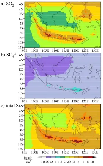
The modeled atmospheric distribution of volcanic S species is shown as annual mean column burden in Fig. 2 as a) SO₂, b) SO2−

4 , and c) total volcanic S (SO2+SO 2₋ 4 ).

The atmospheric concentration of SO₂ is much higher than that of SO2−

4 , and

domi-nates the sum of the two. The annual mean column burden of SO2ranges from 1.5–

5

10 kg (S)/km2 and SO2−

4 from 0–1.5 kg (S)/km 2

. Qualitatively, both SO2 and SO 2−

4

show the highest concentrations near to the volcanoes, while away from the volcanoes the concentration decreases, with the dominant transport away from the volcanoes to-wards the east. Relatively high atmospheric concentrations of the S species is also seen at the northern boundaries of the figures. This is a result of the concentrations

10

of SO₂and SO2−

4 defined at the boundaries of the model domain and is not a result of

the transport of volcanic S.

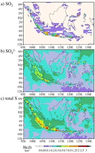
Volcanic S deposition is presented as a) the annual sum of the dry SO2deposition,

b) dry+_{wet SO}2−

4 deposition, and c) the total volcanic S deposition as the sum of the

two (Fig.3). More than 99% of SO2−

4 is deposited via wet deposition, so only the total 15

SO2−

4 deposition is shown. SO2 is dry deposited in large concentrations close to the

volcanoes, up to 3 Mg (S)/km2, but with almost no deposition away from the volcanoes. SO2−

4 , in comparison, has a maximum annual deposition of only up to 1.25 Mg (S)/km 2

, with much more significant deposition away from the volcanoes. Most of the volcanic S is deposited as SO2−

4 (83% of the total S deposition). There is an average

an-20

nual sum of deposition over the entire modeled region of 45.6 kg (S)/km2 SO₂ and 219.6 kg (S)/km2SO2−

4 .

The SO₂ loss rates calculated from the model results (3.2×10−7−4.1×10−5 s−1) agree well in magnitude with SO2loss rates measured at individual volcanoes in other

parts of the world (1.9×10−7₋₅_._4×10−3_s−1_{) (Fig.}₄_{) (}_{Oppenheimer et al.}_,₁₉₉₈_{). There}

25

is a large variability in SO₂loss rates measured at diff_{erent volcanoes, and at Mt. Etna}

(12)

ACPD

5, 11861–11897, 2005

Title Page

Tables Figures

◭ ◮

Back Close

Full Screen / Esc

Print Version

EGU

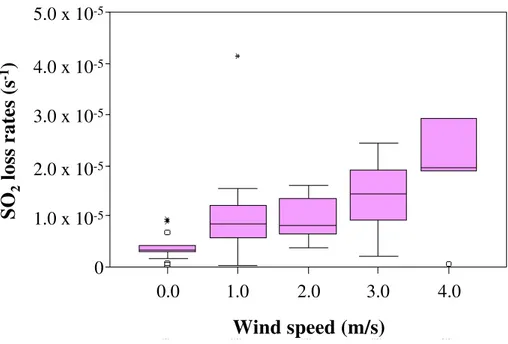
Figure5shows a box plot of the bin wind speed over 1 m/s intervals plotted against SO2 loss rates. The lower edge of the box represents the 25th percentile value and

the upper edge the 75th. The height of each box shows the interquartile range for each season and is an indicator of the variability of the values. The line across the box indicates the median (50th percentile). Four outlayer values are shown as open circles

5

and three extreme values as stars. The correlation between windspeed and SO2loss

rate is weak but statistically significant (p<0.01;R2=₀_._{2). There is a general trend of}

increasing wind speed associated with increased SO2loss rates as well as an increase

in the variability of the SO2 loss rates. Temperature and relative humidity, in contrast,

demonstrate trivial and non-significant (R2<0.02) correlation with SO₂loss rate.

10

SO2 loss rates have been calculated for each season based on the monsoonal

winds: winter monsoon (December–March); spring intermonsoon (April–May) ;

sum-mer monsoon (June–September); fall intermonsoon (October–November). SO2 loss

rates as a function of season are shown as a box plot in Fig.6. Three outlayer values are shown as open circles and one extreme value as a star. Excluding the outlayers and

15

extremes, winter has the lowest variability and spring the highest. The mean seasonal SO₂loss rates for all volcanoes vary between 9.7×10−6s−1(spring) and 1.3×10−5s−1 (summer). A greater variability is demonstrated between individual volcanoes then by the seasonal means over all of the volcanoes.

Loss of volcanic SO₂from the atmosphere can be accomplished via the dry

deposi-20

tion of SO2and by oxidation to SO 2−

4 . There can also be an apparent SO2loss due to

lateral transport outside of the measured plume (in the field) or outside of the predicted transport route (in the calculations performed on the model results). The % of SO₂ lost due to dry deposition and oxidation was calculated by dividing the daily mean dry

deposition of SO2and the annual mean column burden of SO

2−

4 in grid box “V” by the 25

diff_{erence in column burden of SO}₂_{between locations “V” and “V}+_{1”. The remaining}

lost SO2 was attributed to lateral transport. The average for all volcanoes within an

average of 69 km away from the volcanoes is 53% of SO2 lost due to conversion to

SO2−

(13)

ACPD

5, 11861–11897, 2005

Title Page

Tables Figures

◭ ◮

Back Close

Full Screen / Esc

Print Version

EGU

continue at greater distances from the volcanoes. Between locations “V+_{1” and “V}+_2”

(an average distance of 69–121 km from the volcanoes) the sum of the column burden of SO2−

4 and the daily dry deposition of SO2is greater than the loss of SO2.

3.2. “PbCl₂Experiment”

The modeled atmospheric distribution of volcanic PbCl₂is shown as annual mean

col-5

umn burden in Fig. 7. The annual mean column burden of PbCl₂ ranges from 0–

3 g (Pb)/km2. Atmospheric PbCl2is found in greatest concentrations near to the

vol-canoes, with only slight easterly transport. The annual sum of the wet and dry PbCl2

deposition is shown in Fig.8. More than 99% of PbCl₂is deposited via wet deposition, so only the sum of the two is presented. The PbCl2 is deposited in concentrations of 10

up to 2 kg (Pb)/km2with an average annual sum of 52 g (Pb)/km2of PbCl2deposited

in the modeled region.

4. Model result verification

We will assess the quality of the modeling results by comparing the modeled S de-position with the concentration of S measured in peat core samples collected in the

15

modeled region. Peat can serve as a historical record of atmospheric deposition for time periods of up to thousands of years. The peat areas of Indonesia may be par-ticularly useful recorders of the deposition of volcanic emissions because of the large number of historical and modern active volcanoes in the vicinity of peat areas (

Lang-mann and Graf,2003). It has been suggested in several studies that anomalous, high

20

concentrations of S and other chemicals including Pb in peat core samples (collected outside of Indonesia) may be due to volcanic deposition (e.g.Weiss et al.,1997;

Roos-Barraclough et al.,2002;Kylander et al.,2005). Within Indonesia, there are two main types of peat: ombrogenous and topogenous (Page et al.,1999). Ombrogenous peat receives nutrients only from atmospheric deposition while topogenous peat also

(14)

ACPD

5, 11861–11897, 2005

Title Page

Tables Figures

◭ ◮

Back Close

Full Screen / Esc

Print Version

EGU

ceives nutrients from groundwater. Ombrogenous peat is therefore more useful for interpreting the historical deposition of atmospheric compounds. In this work we have taken measurements of S in four ombrogenous peat areas in Indonesia for comparison with the modeled S deposition (Fig.9; Table4). In making this comparison, it is impor-tant to keep in mind that there are other natural sources of S additional to volcanoes,

5

such as vegetation and sea spray, so this comparison can be only qualitative.

The average S of each sampled peat core was calculated by multiplying the average % S in each of the four peat sampling locations with the average peat dry bulk density (0.18 g/cm3) given byShimada et al.(2001). This value was multiplied by the minimum (1.7 mm/yr) and maximum (4.3 mm/yr) peat accumulation rates provided bySupardi

10

et al. (1993), resulting in the presented range of values for the S deposition of each peat core. The average % S was calculated from 3–16 samples within each peat core. Each peat core had measurements of both total S as well as C14 ages, or were very

near to another peat core where C₁₄ age measurements were performed. S values

from portions of the peat cores that were dated to be less than 150 years old were

15

not included in the average as these S values may have been influenced by human activity. The modeled S deposition and the rate of S deposition measured in the peat core samples are of the same order of magnitude. The potential volcanic S contribution to the peat areas ranges from 6–72% of the S measured in the peat samples (Table4). There is a relatively uniform concentration of of volcanic S predicted to be deposited on

20

all four peat areas (215–285 kg/km2−yr). This is because of the distance between the peat areas and the nearest volcanoes (minimum 153 km). It would be helpful to be able to compare the model results with a peat sample collected nearer to the volcanoes, but we have not been able to find such a sample. We find the agreement in scale to be a strong indication that the modeled deposition of the volcanic S is reasonable and feel

25

(15)

ACPD

5, 11861–11897, 2005

Title Page

Tables Figures

◭ ◮

Back Close

Full Screen / Esc

Print Version

EGU

5. Discussion

We will interpret the modeling results and discuss how these results can be used to address the two questions described above: 1) How do variable meteorological condi-tions influence volcanic SO₂concentration in the atmosphere and SO₂loss rates? and 2) How do the transport and deposition patterns of other volcanic compounds relate to

5

SO2?

5.1. SO2loss rate

Temperature, relative humidity, and wind speed have been plotted against the relative % of SO2 lost due to the dry deposition of SO2, oxidation to SO

2−

4 , and lateral

trans-port outside of the predicted plume pathway to see if there is any correlation between

10

variations in the meteorological conditions and the manner in which SO₂ is lost. No such correlation was found. There is an observable seasonal cycle of SO2 loss rates

with the lowest loss rates in spring and the highest in summer. The only seasons with outlayers and extreme values are summer and winter – the monsoon seasons – which are distinguished by strong winds. The model results suggest, albeit weakly, that there

15

may be a relationship between stronger winds and greater SO2 loss rates. There is

a stronger relationship revealed between stronger winds and greater variability of SO₂ loss rates.

The large variabilities of SO2loss rates measured at individual volcanoes have been

attributed to variable atmospheric and plume conditions (Oppenheimer et al., 1998).

20

The results of this study suggest a refinement of this assessment, in that the meteoro-logical condition most significantly influencing the variability of SO2loss rates is wind

speed. It may be more diffi_{cult to obtain a representative SO}₂ _{loss rate for a given}

volcano that is susceptible to highly variable wind conditions, as opposed to a vol-cano that is exposed to more consistent winds. Further fieldwork-based research that

25

(16)

ACPD

5, 11861–11897, 2005

Title Page

Tables Figures

◭ ◮

Back Close

Full Screen / Esc

Print Version

EGU

SO₂ loss rates. If there is indeed such a relationship, it may be important to consider wind speed variations when making interpretations about changes in volcanic activity based on remote SO2measurements. Some variations in SO2flux observed over time

at one volcano may be due to diff_{erences in the winds, as opposed to variations in the}

volcanic emissions.

5

5.2. Diff_{erences in transport and deposition patterns due to solubility}

Both the atmospheric burden and deposition of Pb are three orders of magnitude less than that of S. In both experiments, deposition is relatively uniform with relation to distance from any given volcano and not very distinctive for individual volcanoes. This uniformity is a result of the assumption of an even distribution of the continuous

vol-10

canic emissions between the active volcanoes. PbCl2is rapidly deposited very close to

the volcanoes, resulting in high local concentrations and a sharp decline in deposition at greater distances from the volcanoes. SO2, on the other hand, is much less soluble

in rain than PbCl2. The less soluble SO2has some dry deposition, but is mostly

trans-ported away from the volcanoes prior to conversion to water-soluble SO2−

4 . The SO2 15

that is deposited, however, is deposited at heavier concentrations near to the volcanoes than the PbCl2. Because most of the SO2is converted to SO4

2−_{rather than deposited}

directly as SO₂, there is a much less steep gradient of S deposition at increasing dis-tance from the volcanoes compared with PbCl2, as well as a higher concentration of S

deposition at greater distances from the volcanoes.

20

The influence of solubility on deposition patterns is illuminated by comparing the results of the two performed experiments (Fig.10). The strong dependency of deposi-tion rate on solubility has implicadeposi-tions for the accurate extrapoladeposi-tion of measurements

of SO₂ flux in aged volcanic plumes to other compounds. The further away from a

volcano such measurements are made, the less accurate it is to assume that the

con-25

centration of volcanic SO2measured there has the same ratio to more soluble species

as the ratio measured in fumarolic gases.

(17)

ACPD

5, 11861–11897, 2005

Title Page

Tables Figures

◭ ◮

Back Close

Full Screen / Esc

Print Version

EGU

as the PbCl₂is deposited (Fig.11). Figure11is a box plot with the same specifics as for Figs.5and6. Four outlayer values are shown as open circles at location “V”. The interquartile range increases at greater distance from the volcanoes indicating that the variability of the [PbCl₂]/[SO₂] ratio is growing at greater distances from the volcanoes. The median [PbCl2]/[SO2] ratio decreases exponentially at greater distances from the 5

volcanoes with the mean exponential rate of decay of the [PbCl2]/[SO2] ratio based on

these three distances being y=_106.5e−0.002x

where:

y=_[PbCl₂_]/[SO₂_{] (µg}_/_g)

x=_{distance from volcanoes (km).}

10

The mean [PbCl₂]/[SO₂] ratio at the three distances are: “V” = _{107.7; “V}+_1” =_89.3;

and “V+_2”=_{83.2 µg}_/_g.

Based on this mean rate of decay, we estimate that calculations (e.g. based on COSPEC measurements) which assume a constant [X]/[S] ratio as found in fumarolic gases will result in a 6% overestimation of the atmospheric concentration of highly

15

soluble species at 30 km distance away from the volcano. The overestimation grows at further distances from the volcano.

6. Conclusions

This study demonstrates that realistic modeling of volcanic emissions can lead to an improved understanding of the atmospheric processes occurring in the vicinity of

ac-20

tive volcanoes. The results of the study demonstrate that SO2 loss rates are weakly

correlated with wind speed and uncorrelated with relative humidity or temperature and that there is no correlation between these three meteorological phenomena and the relative amount of SO2 lost due to the dry deposition of SO2, conversion to SO

2−

4 , or

lateral transport. A relationship is shown between increased wind speed and increased

25

(18)

ACPD

5, 11861–11897, 2005

Title Page

Tables Figures

◭ ◮

Back Close

Full Screen / Esc

Print Version

EGU

loss rates as variations in wind speed might lead to changes in SO₂ loss rates inde-pendent of a change in the state of volcanic activity.

The solubility of volcanic emissions is shown to control if they are deposited near to the volcanoes or transported prior to deposition. Highly soluble species such as PbCl2 have high deposition rates near to the volcanoes while the relatively insoluble 5

SO2is transported away from the volcanoes until it is oxidized to SO 2−

4 and then rapidly

deposited. The ratio of [X]/[SO2], with “X” being a soluble species, decreases

expo-nentially at greater distances from the volcanoes. We therefore recommend that the influence of diff_{erent solubilities of volcanic species on atmospheric loss should be}

con-sidered when relating measurements of atmospheric SO2to other volcanic emissions. 10

Acknowledgements. We thank E. Marmer, A. Heil, P. Wetzel, and P. Weis for much help and discussion and for internally reviewing the manuscript. We also thank the German Climate Computing Center (DKRZ) for computer time to run these experiments. MAP was funded by a stipend from the Ebelin and Gerd Bucerius ZEIT Foundation through the International Max Planck Research School on Earth System Modeling.

15

References

Andres, R. J. and Kasgnoc, A. D.: A time-averaged inventory of subaerial volcanic sulfur emis-sions, J. Geophys. Res., 103(D19), 25 251–25 261, 1998. 11863,11884

Bardintzeff, J.-M. and McBirney, A. R.: Volcanology, second edition, Jones and Bartlett, 2000.

11863

20

Bluth, G. J. S., Casadevall, T. J., Schnetzler, C. C., Doiron, S. D., Walter, L. S., Krueger, A. J., and Badruddin, M.: Evaluation of sulfur dioxide emissions from explosive volcanism: the 1982–1983 eruptions of Galunggung, Java, Indonesia, J. Volcan. Geotherm. Res., 63, 243– 256, 1994. 11884

Chang, J. S., Brost, R. A., Isaksen, S. A., Madronich, S., Middleton, O., Stockwell, W. R., and

25

(19)

ACPD

5, 11861–11897, 2005

Title Page

Tables Figures

◭ ◮

Back Close

Full Screen / Esc

Print Version

EGU Lide, D. R. and Frederikse, H. P. R. (Eds.): CRC Handbook of Chemistry and Physics, CRC

Press, 1993. 11870

Delmelle, P.: Environmental impacts of tropospheric volcanic gas plumes, in: Volcanic De-gassing, edited by: Oppenheimer, C., Pyle, D. M., and Barclay, J., London, Geol. Soc. Lon., Special Publication, 213, 381–399, 2003. 11870

5

Esterle, J. S. and Ferm, J. C.: Spatial variability in modern tropical peat deposits from Sarawak, Malaysia and Sumatra, Indonesia: analogues for coal, Int. J. Coal Geol., 26, 1–41, 1994.

11886,11895

Graf, H. F., Feichter, J., and Langmann, B.: Volcanic sulfur emissions: Estimates of source strength and its contribution to the global sulfate distribution, J. Geophys. Res., 102(D9),

10

10 727–10 738, 1997. 11863

Halmer, M. M., Schmincke, D. J., and Graf, H.-F.: The annual volcanic gas input into the atmo-sphere, in particular into the stratosphere: A global data set for the past 100 years, J. Volcan. Geotherm. Res., 115, 511–528, 2002. 11883

Heil, A., Langmann, B., and Aldrian, E.: Indonesian peat and vegetation fire emissions: Study

15

on factors influencing large-scale smoke haze pollution using a regional atmospheric chem-istry model, Mit. and Adapt. Strat. for Glob. Ch., in press, 2005. 11895

Hilton, D., Fischer, T. P., and Marty, B.: Noble gases and volatile recycling at subduction zones, in: Reviews in Mineralogy & Geochemistry – Noble Gases in Geochemistry and Cosmo-chemistry, edited by: Porcelli, D., Ballentine, C. J., and Weiler, R., 47, Washington D.C., Min.

20

Soc. Am., 319–370, 2002. 11865,11883

Hinkley, T. K., Lamothe, P. J., Wilson, S. A., Finnegan, D. L., and Gerlach, T. M.: Metal emis-sions from Kilauea, and suggested revision of the estimated worldwide metal output by qui-escent degassing of volcanoes, Earth Plan. Lett., 170, 315–325, 1999. 11865,11885

Jacob, D.: A note to the simulation of the annual and inter-annual variability of the water budget

25

over the Baltic Sea drainage basin, Met. Atmos. Phys., 77, 61–73, 2001. 11866

Kylander, M. E., Weiss, D. J., Mart´inez Cort´izas, A., Spiro, B., Garcia-Sanchez, R., and Colesab, B. J.: Refining the pre-industrial atmospheric Pb isotope evolution curve in Eu-rope using an 8,000 year old peat core from NW Spain, Earth Plan. Sci. Lett., in press, 2005.

11873

30

Langmann, B.: Numerical modelling of regional scale transport and photochemistry directly together with meteorological processes, Atmos. Environ., 34, 3585–3598, 2000. 11866

(20)

ACPD

5, 11861–11897, 2005

Title Page

Tables Figures

◭ ◮

Back Close

Full Screen / Esc

Print Version

EGU the contribution from volcanic sulfur emissions, Geophys. Res. Lett., 30(11), 1547,

doi:10.1029/2002GL016646, 2003. 11873

LeGuern, F.: Les d ´ebits de CO₂ et de SO₂ volcaniques dans l’atmosph `ere, Bull. Volcanol., 45(3), 197–202, 1982. 11884

Majewski, D.: The Europa Modell of the Deutscher Wetterdienst, Sem. Proc. ECMWF, 2, 147–

5

191, 1991. 11866

McGonigle, A. J. S. and Oppenheimer, C.: Optical sensing of volcanic gas and aerosol emis-sions, in: Volcanic Degassing, edited by: Oppenheimer, C., Pyle, D.M., and Barclay, J., London, Geol. Soc. Lon., Special Publication 213, 149–168, 2003.

Mellor, B. and Yamada, T.: A hierarchy of turbulence closure models for planetary boundary

10

layers, J. Atmos. Sci., 31, 1791–1806, 1974. 11866

Newhall, C. G. and Self, S.: The volcanic explosivity index (VEI): An estimate of explosive magnitude for historical volcanism, J. Geophys. Res., 87, 1231–1238, 1982. 11868

Nho, E.-Y., Le Cloarec, M.-F., Ardouin, B., and Tjetjep, W. S.: Source strength assessment of volcanic trace elements emitted from the Indonesian arc, J. Volcan. Geotherm. Res., 74,

15

121–129, 1996. 11867,11883,11884,11885

Oppenheimer, C., Francis, P., and Stix, J.: Depletion rates of sulfur dioxide in tropospheric volcanic plumes, Geophys. Res. Lett., 25(14), 2671–2674, 1998. 11869, 11871, 11875,

11890

Page, S. E., Rieley, J. O., Shotyk, Ø. W., and Weiss, D.: Interdependence of peat and vegetation

20

in a tropical peat swamp forest, Phil. Trans. R. Soc. Lond., B, 354, 1885–1897, 1999. 11873

Pyle, D. M. and Mather, T. A.: The importance of volcanic emissions for the global atmospheric mercury cycle, Atmos. Environ., 37, 5115–5124, 2003. 11865

Roeckner, E., Arpe, K., Bengtsson, L., Christoph, M., Claussen, M., Duemenis, L., Esch, M., Giorgetta, M., Schlese, M., and Schulzweida, U.: The atmospheric general circulation model

25

ECHAM-4: Model description and simulation of present-day climate, MPI Rep., 218, Ham-burg, Germany, 1996. 11866

Roos-Barraclough, F., Martinez-Cortizas, A., Garc´ia-Rodeja, E., and Shotyk, W.: A 14,500 year record of the accumulation of atmospheric mercury in peat: Volcanic signals, anthropogenic influences and a correlation to bromine accumulation, Earth. Plan. Sci. Lett., 202, 435–451,

30

2002. 11873

(21)

ACPD

5, 11861–11897, 2005

Title Page

Tables Figures

◭ ◮

Back Close

Full Screen / Esc

Print Version

EGU Shimada, S., Takahashi, H., Haraguchi, A., and Kaneko, M.: The carbon content

characteris-tics of tropical peats in Central Kalimantan, Indonesia: Estimating their spatial variability in density, Biogeochem., 53, 3, 249–267, 2001. 11874

Simkin, T. and Siebert, L.: Volcanoes of the World, 2nd ed., Geoscience Press in association with the Smithsonian Institution Global Volcanism Program, Tucson AZ, 1994. 11863,11866,

5

11867,11868

Smolarkiewitz, P. K.: A simple positive definite advection scheme with small implicit diffusion, Month. Weath. Rev., 111, 476–479, 1983. 11866

Spiro, P. A., Jacob, D. J., and Logan, D. J.: Global inventory of sulfur emissions with 1◦ ×1◦ resolution, J. Geophys. Res., 97, 6023–6036, 1992. 11883

10

Stockwell, W. R., Middleton, P., Chang, J. S., and Tang, X.: The second generation regional acid deposition model: Chemical mechanism for regional air quality modeling, J. Geophys. Res., 95, 16 343–16 367, 1990. 11866

Stoiber, R. E., Malinconico Jr., L. L., and Williams, S. N.: Use of the correlation spectrometer at volcanoes, in: Forecasting Volcanic Events, edited by: Tazieff, H. and Sabroux, J.-C.,

15

Elsevier, 1983. 11864

Supardi, Subekty, A. D., and Neuzil, S. G.: General geology and peat resources of the Siak Kanan and Bengkalis Island peat deposits, Sumatra, Indonesia, in: Modern and Ancient Coal-Forming, edited by: Cobb, J. C. and Cecil, C. B., Environments, Boulder, CO, Geol. Soc. Am., Special Paper 286, 1993. 11874,11886,11895

20

Symonds, R. B., Rose, W. I., Reed, M. H., Lichte, F. E., and Finnegan, D. L.: Volatilization, transport and sublimation of metallic and non-metallic elements in high temperature gases at Merapi Volcano, Indonesia, Geoch. Cosmoch. Acta, 51, 2083–2101, 1987. 11885

Textor, C., Graf, H.-F., Herzog, M., and Oberhuber, J. M.: Injection of gases into the stratosphere by explosive volcanic eruptions, J. Geophys. Res., 108(D19), 4606,

25

doi:10.1029/2002JD002987, 2003. 11863

Tiedtke, M.: A comprehensive mass flux scheme for cumulus parameterization in large-scale models, Month. Weath. Rev., 117, 1778–1800, 1989. 11866

Directorate of Volcanology and Geological Hazard Mitigation of Indonesia,http://www.vsi.esdm.

go.id/mvo/mvomonitoring.html, 2005. 11884

30

Walcek, C. J. and Taylor, G. R.: A theoretical method for computing vertical distributions of acidity and sulfate production within cumulus clouds, J. Atmos. Sci, 43, 339–355, 1986.

(22)

ACPD

5, 11861–11897, 2005

Title Page

Tables Figures

◭ ◮

Back Close

Full Screen / Esc

Print Version

EGU Weibring, P., Swartling, J., Ednre, H., Svanberg, S., Caltabiano, T., Condarelli, T., Cecchi,

G., and Pantani, L.: Optical monitoring of volcanic sulphur dioxide emissions – comparison between four different remote-sensing spectroscopic techniques, Opt. Laser Eng., 37, 267– 284, 2002. 11865

Weiss, D., Shotyk, W., Cheburkin, A. K., Gloor, M., and Reese, S.: Atmospheric lead deposition

5

from 12,400 to ca. 2,000 yrs BP in a peat bog profile, Jura Mountains, Switzerland, Water Air Soil Poll., 100, 311–324, 1997. 11873

Weiss, D., Shotyk, W., Rieley, J., Page, S., Gloor, M., Reese, S., and Martinez-Cortizas, A.: The geochemistry of major and selected trace elements in a forested peat bog, Kalimantan, SE Asia, and its implications for past atmospheric dust deposition, Geoch. Cosmoch. Acta,

10

66, 13, 2307–2323, 2002. 11886,11895

Wesley, M. L.: Parameterization of surface resistances to gaseous dry deposition in regional-scale numerical models, Atmos. Environ., 23, 1293–1304, 1989. 11866

W ¨ust, R. A. J. and Bustin, R. M.: Low ash peat deposits from a dendritic, intermontane basin in the tropics: A new model for good quality coals, Int. J. Coal Geol., 46, 3-4, 179–206, 2001.

15

11886,11895

Young, S. R., Voight, B., and Duffell, H. J.: Magma extrusion dynamics revealed by high-frequency gas monitoring at Soufri `ere Hills volcano, Montserrat, in: Volcanic Degassing, edited by: Oppenheimer, C., Pyle, D. M., and Barclay, J., London, Geol. Soc. Lon., Special Publication 213, 219–230, 2003. 11864

(23)

ACPD

5, 11861–11897, 2005

Title Page

Tables Figures

◭ ◮

Back Close

Full Screen / Esc

Print Version

EGU

Table 1.Estimates of Indonesian volcanic emissions.

Emission style SO2flux (Gg/yr) Reference

continuous (non-eruptive) 120 Hilton et al.(2002)

continuous (non-eruptive) 210 Spiro et al.(1992)

continuous (non-eruptive) 1600 Nho et al.(1996)

continuous (eruptive) 1900 Nho et al.(1996)

continuous (eruptive+non-eruptive) 3500 sum fromNho et al.(1996) used in this study

sporadic (eruptive) 290 calculated for this study

(24)

ACPD

5, 11861–11897, 2005

Title Page

Tables Figures

◭ ◮

Back Close

Full Screen / Esc

Print Version

EGU

Table 2.SO₂emissions from individual Indonesian volcanoes.

SO₂flux from SO₂flux from emission inventory measurements

Volcano (Gg/yr) (Gg/yr) Reference

Bromo (Tengger Caldera) 47.4 5.1 Andres and Kasgnoc(1998)

Galunggung 47.7 140.5 Bluth et al.(1994)

240.9 Andres and Kasgnoc(1998)

Merapi 55.6 36.5 Dir. of Volcan. and Geol. Haz. Mit. of Indonesia(2005) 51.1 Andres and Kasgnoc(1998)

73.0 LeGuern(1982)

Slamet 45.4 21.2 Nho et al.(1996)

(25)

ACPD

5, 11861–11897, 2005

Title Page

Tables Figures

◭ ◮

Back Close

Full Screen / Esc

Print Version

EGU

Table 3.Pb/S ratios in Indonesian volcanic gases.

Volcano Pb/S (µg/g) Reference

Merapi 420 Nho et al.(1996)

Merapi 35 Symonds et al.(1987)

Papandayan 280 Nho et al.(1996)

Mean 245 the average of the above measurements was applied in this study

(26)

ACPD

5, 11861–11897, 2005

Title Page

Tables Figures

◭ ◮

Back Close

Full Screen / Esc

Print Version

EGU

Table 4.

Comparison of modeled S deposition and peat core samples.

Distance to Measured S Modeled S Reference

Sampling nearest accumulation deposition Volcanic S (% S measured

location volcano (km) (kg/km2−yr) (kg/km2−yr) (%) in peat core)

Riau 153 398–1006 285 28–72

Supardi et al.(1993) Batanghari

River

160 1744–4412 264 6–15

Esterle and Ferm(1994)

Tasek Bera 258 796–2012 215 11–27

W ¨ust and Bustin(2001) Sungai

Seban-gau

396 428–1084 253 23–59

(27)

ACPD

5, 11861–11897, 2005

Title Page

Tables Figures

◭ ◮

Back Close

Full Screen / Esc

Print Version

EGU

(28)

ACPD

5, 11861–11897, 2005

Title Page

Tables Figures

◭ ◮

Back Close

Full Screen / Esc

Print Version

EGU a) SO₂

b) SO₄

2-95E 100E 105E 110E 115E 120E 125E 130E 6N

4N 2N EQ 2S 4S 6S 8S 10S 12S

95E 100E 105E 110E 115E 120E 125E 130E 6N

4N 2N

EQ 2S

4S 6S

8S 10S

12S

95E 100E 105E 110E 115E 120E 125E 130E 6N

4N 2N EQ 2S 4S 6S 8S 10S 12S

c) total S

kg (S)

km2 _{0 0.25 0.5 1 1.5 2 2.5 3 4 6 8 10}

Fig. 2. Annual mean vertical column burden of(a)SO₂,(b)SO2−

4 , and(c)total S: SO2+SO 2−

4

(29)

ACPD

5, 11861–11897, 2005

Title Page Abstract Introduction Conclusions References Tables Figures ◭ ◮ ◭ ◮ Back Close

Full Screen / Esc

Print Version

EGU 95E 100E 105E 110E 115E 120E 125E 130E

6N 4N 2N EQ 2S 4S 6S 8S 10S 12S

95E 100E 105E 110E 115E 120E 125E 130E 6N 4N 2N EQ 2S 4S 6S 8S 10S 12S

95E 100E 105E 110E 115E 120E 125E 130E 6N 4N 2N EQ 2S 4S 6S 8S 10S 12S kg (S)

km2 _{0 0.25 0.5 1 1.5 2 2.5 3 4 6 8 10} kg (S)

km2 kg (S)

km2 _{0 0.25 0.5 1 1.5 2 2.5 3 4 6 8 10}_{0 0.25 0.5 1 1.5 2 2.5 3 4 6 8 10} 95E 100E 105E 110E 115E 120E 125E 130E 6N 4N 2N EQ 2S 4S 6S 8S 10S 12S a) SO₂

b) SO₄2- 95E 100E 105E 110E 115E 120E 125E 130E 6N 4N 2N EQ 2S 4S 6S 8S 10S 12S

95E 100E 105E 110E 115E 120E 125E 130E 6N 4N 2N EQ 2S 4S 6S 8S 10S 12S

c) total S

95E 100E 105E 110E 115E 120E 125E 130E Mg (S)

km2 Mg (S)

km2 _{0 0.05 0.1 0.2 0.3 0.5 0.7 0.9 1.25 2 2.5 3}_{0 0.05 0.1 0.2 0.3 0.5 0.7 0.9 1.25 2 2.5 3} 6N 4N 2N EQ 2S 4S 6S 8S 10S 12S

Fig. 3. Annual sum of the(a)dry SO₂deposition,(b)dry+wet SO2−

4 deposition, and(c)total

S: dry SO₂+_dry+_{wet SO}2−

(30)

ACPD

5, 11861–11897, 2005

Title Page Abstract Introduction Conclusions References Tables Figures ◭ ◮ ◭ ◮ Back Close

Full Screen / Esc

Print Version

EGU

1.0 x 10-7

1.0 x 10-6

1.0 x 10-5

1.0 x 10-4

1.0 x 10-3

1.0 x 10-2

1000 10000 100000

Height (volcano/plume; m)

S O2 lo ss r a te s (s -1 )

Indonesian volcanoes- this study Pinatubo

Redoubt Mt. St. Helens Nyamuragira Mt. Etna Mt. Erebus Soufriere Hills

1.0 x 10-7

1.0 x 10-6

1.0 x 10-5

1.0 x 10-4

1.0 x 10-3

1.0 x 10-2

1000 10000 100000

Height (volcano/plume; m)

S O2 lo ss r a te s (s -1 )

Redoubt Mt. St. Helens Nyamuragira Mt. Etna Mt. Erebus Soufriere Hills

Redoubt Mt. St. Helens Nyamuragira Mt. Etna Mt. Erebus Soufriere Hills ❹❺❶✍❸ ❹❜❶P❸

Fig. 4. Modeled SO₂ loss rates (yellow squares) are plotted against the actual height of each volcano and measured SO₂loss rates fromOppenheimer et al.(1998) are plotted against the observed plume height.

(31)

ACPD

5, 11861–11897, 2005

Title Page

Tables Figures

◭ ◮

Back Close

Full Screen / Esc

Print Version

EGU

0.0

1.0 2.0 3.0

4.0 Wind speed (m/s)

5.0 x 10

-5

4.0 x 10

-5

3.0 x 10

-5

2.0 x 10

-5

1.0 x 10

-5

0 SO

2

lo

ss r

a

te

s (

s

-1

)

(32)

ACPD

5, 11861–11897, 2005

Title Page

Tables Figures

◭ ◮

Back Close

Full Screen / Esc

Print Version

EGU

4.0 x 10

-5

3.0 x 10

-5

2.0 x 10

-5

1.0 x 10

-5

0 Winter Spring Summer Fall

Season

S

O

2

lo

ss

r

a

te

s

(s

-1

)

(33)

ACPD

5, 11861–11897, 2005

Title Page

Tables Figures

◭ ◮

Back Close

Full Screen / Esc

Print Version

EGU

(34)

ACPD

5, 11861–11897, 2005

Title Page

Tables Figures

◭ ◮

Back Close

Full Screen / Esc

Print Version

EGU

(35)

ACPD

5, 11861–11897, 2005

Title Page

Tables Figures

◭ ◮

Back Close

Full Screen / Esc

Print Version

EGU

Fig. 9.Peat sampling locations on a map of the fractional peat coverage of the modeled region (afterHeil et al.,2005). 1 W ¨ust and Bustin(2001); 2Weiss et al.(2002); 3 Esterle and Ferm

(36)

ACPD

5, 11861–11897, 2005

Title Page

Tables Figures

◭ ◮

Back Close

Full Screen / Esc

Print Version

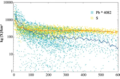
EGU S

Pb * 4082 S

Pb * 4082

Distance from nearest volcano (km)

0 100 200 300 400 500 600 10000

1000

100

10

1

k

g

[X

]/k

m

2

(37)

ACPD

5, 11861–11897, 2005

Title Page

Tables Figures

◭ ◮

Back Close

Full Screen / Esc

Print Version

EGU V V+1 V+2

0 69 121 0.2

0.1

0

Average distance (km)

PbCl

2

/S

O

2