A Parallel Processing Algorithms for Solving Factorization
and Knapsack Problems
G. Aloy Anuja Mary 1 , J.Naresh2 and C.Chellapan3
1,2Research Scholar,Department of Computer Science & Engineering, College of Engineering, Guindy
Anna University, Chennai-600025
3
Professor,Department of Computer Science & Engineering, College of Engineering, Guindy Anna University, Chennai-600025
Abstract
Quantum and Evolutionary computation are new forms of computing by their unique paradigm for designing algorithms.The Shor’s algorithm is based on quantum concepts such as Qubits, superposition and interference which is used to solve factoring problem that has a great impact on cryptography once the quantum computers becomes a reality. The Genetic algorithm is a computational paradigm based on natural evolution including survival of the fittest, reproduction, and mutation is used to solve NP_hard knapsack problem. These two algorithms are unique in achieving speedup in computation by their adaptation of parallelism in processing.
Keywords: Quantum computing, Qubits, superposition, mutation, parallesim.
1.
Introduction
In 1965, computer chip pioneer Gordon E.Moore noticed that transistor density in chips had doubled every year in the early 1960s, and he predicted that this trend would continue. This prediction moderated to a doubling every 18 month’s and extended to computer speed is known as Moore’s law. It has held remarkably well for 40 years. Moore’s law will stop doubling the speed of our computers within a decade, when chips hit atomic scale. Then the progress depends on algorithmic ingenuity or on novel ideas such as quantum and evolutionary computing [3].
Quantum computing is the attracting one since its superiority was demonstrated by a few quantum algorithms such as Shor’s quantum factoring algorithm and Grover’s database search algorithm. Shor’s algorithm finds the prime factors of an n-digit number in polynomial time while best known classical algorithm require exponential time. Multiplying two prime numbers together is a very simple process. Factorizing the result back into its two primes, however, is currently still a very time consuming process on classical computers. This result is the basis of the well known cryptographic algorithm RSA. It has been suggested that quantum computers, if ever built, will have the power to reverse this result and to be able to factorize numbers in a shorter time than it would take to multiply them together in the first place, hence making RSA obsolete. In a classical computer, a bit is simply the basic measure of information. It can hold either a 1 or a 0. Similarly
the basic measure of information in a quantum computer is a qubit which have the two possible values 1 and 0, but also with the superposition of the two basis states [4].Equation (1) represents the qubit state ψ as a linear combination of the |0 > and |1 > states.
| ψ > = α |0 > + β |1 > (1)
Where α and β are the complex numbers that specify the probability amplitudes of the corresponding states. Therefore the paper adopts MATLAB for simulation of the Shor’s quantum algorithm to solve factoring problem.
Secondly, Genetic algorithm is a kind of computational model in evolutionary computing and new global optimization search algorithm that simulates the biology evolving process [5]. The Knapsack is a combinatorial optimization problem. Given a set of item Xi, each with a value Vi, and weight Wi, the objective is to maximize value of the backpack subject to a weight limit. The mathematical formulation of the problem is as follows
n Maximize ∑Vi Xi
i=1 (2) n
S.T. ∑ Wi Xi i=1
Xi= 0 or 1, j=1,2,…, n.
This paper adopts java language to program the Genetic algorithm to solve NP_Complete Knapsack problem.
This paper is organized as follows. Section 2 describes complexity classes of factoring and Knapsack problem. Section 3 and 4 describes Shor’s and Genetic algorithm respectively. Section 5 and 6 simulates the experiment Shor’s algorithm for factoring and Genetic algorithm for Knapsack problem respectively. Concluding remarks follow in section 7.
Computer Scientists categorize problem according to how many computational steps it would take to solve a large example of the problem using the best algorithm known. The problems are grouped into broad overlapping classes based on their difficulty. Three of the most important classes are as follows.
P PROBLEMS: Ones computers can solve efficiently in polynomial time.
NP PROBLEMS: Ones whose solution are easy to verify.
NP_COMPLETE PROBLEMS: An efficient solution to one would provide an efficient solution to all NP challenges.
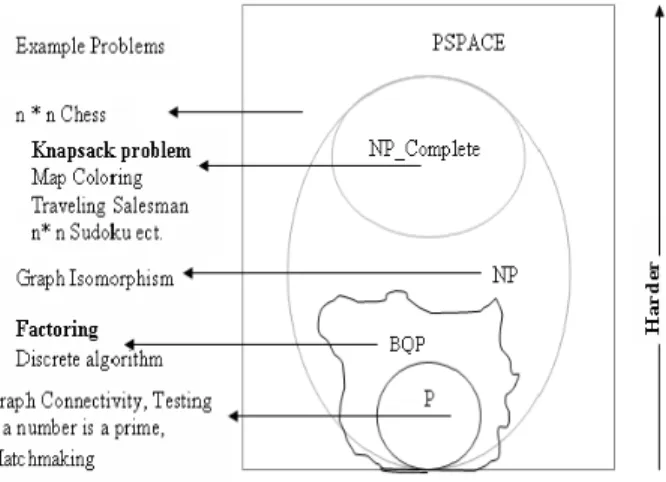
A fourth class of problems that quantum computers would solve efficiently (BQP) is related to these fundamental classes of computational problems as shown in fig.
The BQP (the letter stand for bounded _error, quantum polynomial time) includes all the P problems and also a few other NP problems. Finally PSPACE problems are those that a conventional computers can solve using only a polynomial amount of memory but possibly requiring an exponential number of steps[3]. After knowing about complexity classes, the Knapsack problem is mapped to NP_Complete and Factoring problem is mapped to BQP as shown in fig 1.
Fig 1 Complexity Classes
3.
SHOR’S Algorithm
Given a number N, constructed from the multiplication of two distinct but unknown prime numbers, the goal is to find what the two prime factors were. Shor showed how to turn factorization into the problem of order finding, using a quantum subroutine, the order of a function in polynomial time.
Shor took advantage of a fundamental result from number theory. Given two numbers x and N which are co-prime to
each other, the function F (k) = xk (MOD N) is periodic with some period r such that
F(k)=xk(MODN)=xk+r(MODN) (3)
Hence, this implies that
xr≡1 (MOD N) (4)
If r is an even integer, then the following algebraic manipulation produces
(xr/2)2 ≡ 1 (MOD N) (5) (xr/2)2 -1 ≡ 0 (MOD N) (6) (xr/2 -1) (xr/2 +1 ) ≡ 0 (MOD N) (7)
This means that (xr/2 -1) (xr/2 +1) is an integer multiple of N and so long as xr/2 ≠ ±1 then at least one of (xr/2 -1) and (xr/2 +1) must have a nontrivial factor in common with N.
Hence, by computing the gcd (xr/2 -1, N) and gcd (xr/2 +1, N) the factor of N can be obtained.
Shor’s algorithm can thus be broken up into three distinct sections.
A. Classical pre-processing: pick a number x,
co-prime to N
B. Quantum computation: Find the order r, such
that xr≡ 1(M OD N)
C. Classical post-processing: If r is even, calculate
the two possible factors of N.
The trick Shor used in order to achieve the parallelism offered by quantum mechanics was to notice that it is possible to perform both the modular exponentiation of a quantum register followed by finding the corresponding period of the function, in single quantumly parallel operations.
A. Classical Pre-Processing
Step 1 Check whether N is of the form N= (prime)α or N=
2 (prime)α where α € {0,1,2, …}, if true then there are efficient classical algorithms which can be used, else go to step 2.
Step 2 Choose a random number x such that 1<X<N-1 and
which is relatively prime to N.
Step 3 Find an integer q which is a power of 2 and satisfies
the condition n2 <=q<=2 n2 where n= 2[log N].
Step1 Initialization of the quantum registers
Initialize two quantum registers |Reg1, Reg2> such that Reg1 has n qubits and Reg2 has ֩log N ֪ qubits. Reg1 will hold the possible k’s and Reg2 will hold the respective F (k) values. Once the qubit registers space are assigned, both are initialized to the 0 state |0, 0>
Step 2 Place Reg1 into a superposition of all possible states
Once the two register quantum state is set up, the Reg1 is placed into an equally weighted superposition of all the integers from 0 to q − 1. This would then leave the quantum memory registers in the state
(8)
A calculation performed on a quantum register is actually a calculation performed on every possible value that register can represent all at the same time. This is what allows the improvements in speed compared to classical algorithms.
Step 3 Place xReg1 (MOD N ) in Reg2
Next apply the function F (k) = xk (M OD N) to Reg1, storing the result in Reg2. Due to quantum parallelism this will only take one step. The state of the registers after this step will be
(9)
Now measure the second register. The value stored there will collapse to give us only a single value, K. This measurement also has the effect of collapsing register 1 in such a way that if measuring register 1 next, one would observe all possible corresponding i’s with equal probability and any i such that xi (M OD N ) ≠ K would have zero probability of being seen. If A denotes the set of values from Reg1 which satisfy this new condition, and ||A|| is the number of states it contains, the state of our registers would then be
(10)
Where r is the period of F, j is the index over A and s < r is the initial random offset such that xs (M OD N) = K. As this collapse of the state takes place in one instantaneous step, it shows the power which quantum superposition is able to employ.
Unfortunately, directly extracting r or a multiple of it from the above state due to the random offset s is not possible. Hence, to get around this problem the Discrete Fourier Transform
(DFT) of Reg1 is taken. This is due to the fact that the probability spectrum of the transformed state is invariant to the offset [4].
Step 4 Calculation of the period r
The DFT of a state φ results in the following register state
(11)
This transform can actually be performed in a single step on a quantum computer using quantum parallelism. Therefore by taking the DFT of Reg1, results in the state of our system then being
(12)
Measuring the state of Reg1 will now collapse the register to a single value which is called m. It is not possible to extract any other information from the register, such as the number of states which have peak probability, as once it has been measured it collapses to a single value thereafter. The measured value has a very high probability of being an integer multiple, λ, of q/rwhere r is our desired period.
The final step of calculating r is to convert our calculated value of m/q from a decimal floating point value to a rational number. We ensure that both the numerator and denominator are kept to values less than q. There is an efficient classical algorithm for solving this problem using continued fractions but this analysis has been omitted because MATLAB has an inbuilt function for performing the task when implementing the algorithm.
A final note to make here is that our approximation numerator/denominator≈λ/r is only valid when gcd(λ, r) = 1, since the rational form is not unique. This again is incorporated into the MATLAB function, which finds the rational approximation in its simplest form.
C. Classical Post-Processing
At this stage of the algorithm, the period r of random number x is found. If r is odd, then unfortunately this is of no help, so discard it and go back to the beginning and choose a new random number to use as our x.
Assuming that eventually do find an r which in even, we calculate
Then use these values to test whether they are our chosen factors by multiplying them together. If they turn out to be nontrivial numbers which when multiplied together equals N, factoring is done. Otherwise, we need to re-run the algorithm choosing a new value of x to use.
There is a very high probability that after only O (log N) runs of the algorithm, the two unique factors which produce our number N will be found.
4.
Description of Genetic Algorithm
Genetic algorithms are a part of evolutionary computing, which inspired by Darwin’s theory about evolution. The solution to a problem a problem solved by Genetic algorithm is evolved from large search space. GA uses operators inspired by evolutionary biology such as mutation, selection and crossover. And have two basic parameters crossover probability and mutation probability beside the population size. The structure of simple GA is shown in Fig 2.
Fig 2 Structure of Genetic Algorithm
The design of GA that solves knapsack problem is as follows
Step 1 Choose binary coding to represent items, a selection operator, a crossover operator, and a mutation operator. Choose population size n, crossover probability pc and mutation probability pm. Initialize a random population of string l. Choose a maximum allowable generation number t max. Set t=0.
Step 2 Evaluate each string in the population.
Step 3 If t>t max or 90% of evaluated strings have same fitness value, Terminate.
Step 4 Perform reproduction on the population. Step 5 Perform crossover on random pairs of strings.
Step 6 Perform mutation on every string.
Step 7 Evaluate strings in the new population. Set t=t+1and go to step 3.
5.
Simulate Factorization Problem
Factoring of N=15, provides evidence that implementation works and is able to find the required two prime factors of N = 15. Calculating n and q for this particular N gives us 8 and 256, respectively. Next choose x = 13 randomly, populate Reg1 with 0...q-1, calculate Reg2 = xReg1 (MOD N) and finally determine the probability of seeing each value of Reg1 when the quantum register Reg2 is measured. The state of A is given below, together with the probability of seeing Reg1 once Reg2 has been measured and found to be K = 13.
Table 1 the values held in Reg1 and Reg2 when trying to factorize the Number N =15 using the random number x = 13 [2]
Reg1 Reg2 Prob
before
Prob
after DFT
0 1 0.0625 0 8
1 13 0.0625 0.125 0
2 4 0.0625 0 0
3 7 0.0625 0 0
4 1 0.0625 0 0
5 13 0.0625 0.125 0
6 4 0.0625 0 0
7 7 0.0625 0 0
8 1 0.0625 0 0
9 13 0.0625 0.125 0
. . . . . . . . .
. . . . .
. . . . . . . . . . . . . . . . . . . .
253 13 0.0625 0.125 0
254 4 0.0625 0 0
255 7 0.0625 0 0
Calculating C by dividing the m values by q gives us 0.25, 0.5 and 0.75 as possible values.
Next the rat MATLAB function is used to turn these values of C into rational approximations. The denominator and hence possible values of r are found to be 4, 2 and 4 with corresponding numerators 1, 1 and 3. Finding the greatest common divisors of these xr/2 ± 1 with respect to N ends up producing the correct two factors 5 and 3 which when multiplied together form N = 15.
Fig 3 is a plot showing the DFT values of Reg1 for this particular example.
0 50 100 150 200 250
0 1 2 3 4 5 6 7 8
Probabilities of observing values of c between 0 and 4000
Values of c
DF
T
Figure 3 Plot of DFT graph for N =15 and X = 13
6.
Simulate Knapsack Problem
Assumed n of the goods number is 50 the weight of the goods is {wi} the value of the goods is {vi} and capacity of the Knapsack is c=1000.
{wi}={80,82,85,70,72,70,66,50,55,25,50,55,40,48,50,32,22,6 0,30,32,40,38,35,32,25,28,30,22,25,30,45,30,60,50,20,65,20,2 5,30,10,20,25,15,10,10,10,4,4,2,1};
{vi}={220,208,198,192,180,180,165,162,160,158,155,130,12 5,122,120,118,115,110,105,101,10,100,98,96,95,90,88,82,80, 77,75,73,72,70,69,66,65,63,60,58,56,50,30,20,15,10,8,5,3,1};
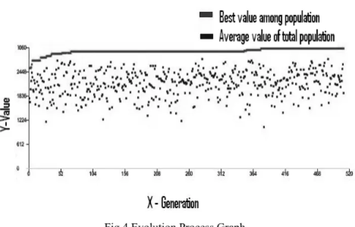
Population size is 10 and maximal evolution generation is 500 in the experiment. Fig 4 shows the evolution process graph of the total value of the selected goods. The x-axis shows the evolution generation and y axis shows the total value of the selected goods. The optimal result of the genetic algorithm corresponds to the value of the Knapsack that is 3063.
Fig 4 Evolution Process Graph
Table 2 Export experiment result, when the evolution process of the Genetic algorithm is over
7.
Conclusion
This paper provides a mathematical description of Shor’s quantum algorithm for factorizing numbers that have been constructed from two primes into their two composite primes. Then Shor’s fast algorithm for factoring based on Fourier transform is simulated on classical computer running MATLAB. The example provided proves that the simulated algorithm indeed is able to factorize numbers. This paper also provides a description of genetic algorithm for solving NP_hard Knapsack problem a kind of combinatorial optimization problem. Then the algorithm is simulated for the example provided running Java language proves that simulated algorithm is able to find global optimization solution. Therefore algorithms based on unique computational paradigms such as quantum and evolutionary computing is stressed for speedup in computation to enable technological development, even when Moore’s law stop’s working in a decade when chips hit atomic scale.
References
[1] Soltanaghaei, M.R., Z.A. Zukarnain,A.Mamat and H.Zainuddin,2009. A hybrid algorithm for finding shortest path in network routing., J.Theor.Applied Inform.Technol.,5:360-364.
[3] Michael A. Nielsen and L. Chuang, Quantum Computation and Quantum information. Cambridge university press, Cambridge, 2000.
[4] P. W. Shor, Polynomial _ time algorithms for prime factorization and discrete logarithms on a quantum computer, SIAM J. Computing 26, pp. 1484-1509, 1997.
[5] Rui Liu, Jin-bo Zhang, Rui-jie Liu, and Ji-xian Li, “On the algorithm of solving the 0_1 knapsack problem based on the Genetic algorithm”, Journal of yunnan nationalities University(Natural Sciences Edition).Vol. 17, No.4, 2008, pp. 377-379
G.Aloy Anuja Mary is a PhD student in the Department of Computer Science and Engineering at Anna University, Chennai, India. She received her B.E Electronics and communication Engineering from Sivanthi Aditanar College of Engineering College under Manonmaniam Sundaranar University in 2003 and M.E Communication Systems from National College of engineering under Anna University in 2005, Chennai, India. Her current research is on Quantum Cryptography and Communication.
J.Naresh is a M.E student in the Department of Computer Science and Engineering at Anna University,Chennai, India. He received his M.Sc(physics) from Sacred Heart College,Tirupathur underMadras University in 2003 and B.Sc(Physics) fromSankara College,Kanchipuram under Madras University in 2000, Chennai, India. His current research is on Quantum computing.
![Table 1 the values held in Reg1 and Reg2 when trying to factorize the Number N =15 using the random number x = 13 [2]](https://thumb-eu.123doks.com/thumbv2/123dok_br/16454162.197757/4.918.478.813.380.903/table-values-trying-factorize-number-using-random-number.webp)