Data Search Algorithms based on Quantum Walk

Data Search Algorithms based on Quantum Walk

Masataka Fujisaki

, Hiromi Miyajima

, Noritaka Shigei

Abstract—For searching any item in an unsorted database with N items, a classical computer takes O(N) steps but Grover’s quantum searching algorithm takes only O(√

N) steps. However, it is also known that Grover’s algorithm is effective only in the case where the initial amplitude distribution of dataset is uniform, but is not always effective in the non-uniform case. In this paper, we propose some quantum search algorithms. First, we propose an algorithm in analog time based on quantum walk by solving the schrodinger equation. The proposed algorithm shows best performance in optimum time. Next, we will apply the result to Grover search algorithm. It is shown that the proposed algorithm shows better performance than the conventional one. Further, we propose the improved algorithm by introducing the idea of the phase rotation. The algorithm shows best performance compared with the conven-tional ones.

Index Terms—quantum search algorithm ; Grover search algorithm; initial amplitude distributions of dataset; observed probability

I. INTRODUCTION

With quantum computation, many studies have been made. Shor’s prime factoring and Grover’s data search algorithms are well known[1], [2], [4]. Further, Ventura has proposed quantum associative memory by improving Grover’s algo-rithm [3], [5]. Data search problem is to find any data effec-tively from unsorted dataset. For searching any item in an

unsorted database withN items, a classical computer takes

O(N)steps, but Grover’s algorithm takes onlyO(√N)steps. However, it is also known that Grover’s algorithm is effective only in the case where the initial amplitude distribution of dataset is uniform, but is not always effective in the non-uniform case[3]. Further, Ventura has proposed the quantum searching algorithm but it is effective only in the special case for the initial amplitude distribution[6], [7]. Therefore, it is necessary to find effective algorithms even in the case where the initial amplitude distribution of dataset is not uniform. For example, associative memory needs non-uniform initial data distribution [3]. In this paper, we propose some quantum search algorithms. First, we propose an algorithm in analog time based on quantum walk by solving the schrodinger equation. The proposed algorithm shows best performance in optimum time. Next, we will apply the result to Grover search algorithm. It is shown that the improved algorithm shows better performance than the conventional one. Further, we propose the algorithm by introducing the idea of the phase rotation[8]. The proposed algorithm shows best performance compared with the conventional ones.

This work is supported by Grant-in-Aid for Scientific Research (C) (No.22500207) of Ministry of Education, Culture, Sports, Science and Technology of Japan.

* Graduate School of Science and Engineering, Kagoshima University, 1-21-40 Korimoto, Kagoshima 890-0065, Japan

†email: k7605487@kadai.jp

‡corresponding author to provide email: miya@eee.kagoshima-u.ac.jp §email: shigei@eee.kagoshima-u.ac.jp

II. PRELIMINARY

The basic unit in quantum computation is a qubitc0|0i+ c1|1i , which is a superposition of two independent states

|0iand|1icorresponding to the states 0 and 1 in a classical

computer, where c0 andc1 are complex numbers such that

|c0|2+|c1|2= 1. We use the Dirac bracket notation, where

the ket|iiis analogous to a column vector. Letnbe a positive

integer and N = 2n_{. A system with n qubits is described}

usingN independent state|ii(0≤i≤N−1) as follows: N−1

∑

i=0

ci|ii (1)

where ci is a complex number, ∑N−1

i=0 |ci|2 = 1 and |ci|2

is the probability of state |ii.The direction of ci on the complex plane is called the phase of state|iiand the absolute value |ci| is called the amplitude of state |ii. In quantum system, starting from any quantum state, the desired state is formed by multiplying column vector of the quantum state by unitary matrix. Finally, we can obtain the desired state with high probability through observation[2]. The problem is how we can find unitary matrix. Grover has proposed the fast data search algorithm. Let us explain the Grover’s algorithm shown in Fig.1. Grover has proposed an algorithm for finding one item in an unsorted database. In the conventional computation, if there are N items in the database, it would

requireO(N)queries to the database. However, Grover has

shown how to perform this using the quantum computation with onlyO(√N)queries[2]. Let ZN ={0,1,· · ·, N−1}. Let us define the following operators.

I_{a = Identity matrix except for}

I_{(a+ 1, a+ 1) =−1, a∈ZN (2)}

which inverts any state|ψiand

W_{(x, y) = √}1

N(−1)

x0y0+_···+xN−1yN−1

forx= N−1

∑

i=0

xi2i, y= N−1

∑

i=0

yi2i, (3)

which is called the Walsh or Hadamard transform and performs a special case of discrete Fourier transform. We begin with the|¯0istate and apply W _{operator to it, where}

|¯0imeans that all states are0and the number of 0’s for¯0is N. As a result, all the states have the same amplitude1/√N. Next, we apply theI_{τ operator, where |τiis the searching}

state. Further, we apply the operator

G₌₋W I₀W ₍₄₎

Followed by the Iτ operator T = (π/4)√N times and

observe the system[2]. G _{operator has been described as}

1. Initial state|ψi

2. |ψi=W_|¯0_i=|¯1_i

3. RepeatT times

4. |ψi=I_τ|ψi

5. |ψi=G_|ψi

6. Observe the system

Fig. 1. Grover search algorithm

one of all states.

Example 1[6]:

Let n= 4 and N = 16. Let searching data |τi =|6i=

|0110i and the number of stored (memorized) data l= 16. Then, the desired data 0110 is obtained with the probability 0.96 by using Grover’s algorithm. We can get the searching data with high probability.

Next, assuming that stored data are|0i,|3i,|6i,|9i,|12i, and|15i, and searching data is|6i, that is l= 6. The initial state |ψiis as follows:

|ψii=

{

1 for anyi of stored date

0 otherwise, (5)

Then, the desired data 0110 is obtained with the probability 0.44. It shows that Grover’s algorithm does not always give a good result in the case where N6=l.

Therefore, it is needed to find effective algorithms even in the case where the initial amplitude distribution of dataset is not uniform.

III. QUANTUM SEARCH IN ANALOG MODEL BASED ON

QUANTUM WALK

1

i1

j1

m-1

0

i0

j0

im-1

jm-1

il-1

l-1 N-1 All the data

l pieces of memorized data

m pieces of search data (stored)

(marked)

Fig. 2. Description of data search problem

In the following, we introduce a quantum search algorithm using analog model of quantum walk. In order to clarify the problem, we will explain the Fig.2. It is assumed that l

pieces of data are memorized (stored) in the system of N

pieces of data. Now we want to find any data inmpieces of data (marked) with high probability. Grover has shown the effective algorithm in the case ofN =l,m= 1(see Fig.1).

A. Schroedinger equation and quantum walk

In this chapter, we propose an algorithm based on quantum walk in analog time model. As the state of system in quantum model is determined by the Schroedinger equation , we can obtain the result by solving the Schroedinger equation under the special condition[9],[10].

The Schroedinger equation for the state of system is represented as follows[9]:

i¯hd|ψi

dt =H|ψi, (6)

where ¯h is Plank constant and H _{is Hamiltonian which}

means all the energy of the system. Then H ₌H† _holds,

whereH† _{is the transposed matrix of complex conjugate for}

H_.

Then the solution is represented by

|ψ(t)i=U_{(t)|ψ(0)i, (7)}

where

U_{(t) = exp(−it}H_{) (8)}

and U_{(t) is called time expansion operation of the state}

and|ψ(0)iis the initial state of system. Therefore, the state

of system is determined by Hamiltonian H_{. Let Pw(t) be}

defined as the observed probability of system at time t as

follows:

Pw(t) =|hw|U_(t)|ψ(0)i|2_{. (9)}

The state of system to search is called the marked one and the other is called the unmarked state. The number of marked states ism(see Fig.2). HamiltonianHρ corresponding to the potential energy is represented by an identity matrix except for

H_{ρ(ji, ji) =−1, (10)}

wherei∈Zm.

Let L _{be the state assignment over the graph. Then the}

HamiltonianH _{of the system is defined using the mobility}

ras follows[9]:

H_=−γL₊H_{ρ (11)}

Let G _{= (}V_,E_{) be the perfect graph to act for system,}

where V _{is the set of vertexes and} E _{is the set of edges.}

ThenL_{is represented as follows:}

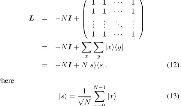
L _{= −N}I₊



   

1 1 · · · 1 1 1 · · · 1

..

. ... . .. ... 1 1 · · · 1



   

= −NI₊∑

x

∑

y

|xihy|

= −NI_{+N|sihs|, (12)}

where

|si=√1

N N−1

∑

x=0

|xi (13)

Finally, HamiltonianH _{is represented as follows:}

H_=γNI_{−γN|sihs|+}H_{ρ (14)}

It is known that any quantum arrives at any place (state)

in O(√N) steps by using quantum walk. Assuming that

the potential energy of the place to arrive is low, the high probability of the state is performed.

Then, letU _{be defined as follows:} U _{= exp(−}1

2itγNI) exp(itA), (15) where

A_{=γN|sihs| −}H_ρ−1

B. Derivation of the time expansion operator U

Let us compute the Eq.(15).

LetC _{be any matrix. Then the following relation holds:}

exp(C_{) =}

∞ ∑ r=0 1 r!C r_. (17)

In order to compute the Eq.(15), Ar _{must be computed.}

Here, in order to understand the computation ofAr_easily, we will consider the case ofN = 8.

Ar₌

           

ζ(r) δ(r) α(r) α(r) δ(r) δ(r) α(r) α(r) β(r) ǫ(r) β(r) β(r) η(r) η(r) β(r) β(r) α(r) δ(r) ζ(r) α(r) δ(r) δ(r) α(r) α(r) α(r) δ(r) α(r) ζ(r) δ(r) δ(r) α(r) α(r) β(r) η(r) β(r) β(r) ǫ(r) η(r) β(r) β(r) β(r) η(r) β(r) β(r) η(r) ǫ(r) β(r) β(r) α(r) δ(r) α(r) α(r) δ(r) δ(r) ζ(r) α(r) α(r) δ(r) α(r) α(r) δ(r) δ(r) α(r) ζ(r)

            (18)

From the relation that Ar+1 _{= A}r_{A and A}1 _{is known,}

the following recursion formula are obtained:

β(r+ 1) =

{

(N−m)γ−1

2

}

β(r)

+(m−1)γη(r) +γǫ(r) (19)

η(r+ 1) = (N−m)γβ(r) +

{

(m−1)γ+1 2

}

η(r)

+γǫ(r) (20)

ǫ(r+ 1) = (N−m)γβ(r) + (m−1)γη(r)

+(γ+1

2)ǫ(r) (21)

α(r+ 1) =

{

(N−m−1)γ−1₂ }

α(r)

+mγδ(r) +γζ(r) (22)

δ(r+ 1) = (N−m−1)γα(r) + (mγ+1 2)δ(r)

+γζ(r) (23)

ζ(r+ 1) = (N−m−1)γα(r) +mγδ(r)

+(γ−1₂)ζ(r) (24)

Now, letv_1(r),v_2(r),K_1andK_{2 be defined as follows:}

v_{1(r) =}

  β(r) η(r) ǫ(r)   (25)

v_{2(r) =}

  α(r) δ(r) ζ(r)   (26)

K_{1 =}





γ(N−m)−12 γ(m−1) γ

γ(N−m) γ(m−1) +1₂ γ γ(N−m) γ(m−1) γ+1₂





(27)

K_{2 =}





γ(N−m−1)−12 γm γ

γ(N−m−1) γm+1₂ γ γ(N−m−1) γm γ−12





(28)

Then, the following relation hold:

v_{1(r+ 1) =}K₁v_{1(r) (29)} v_{2(r+ 1) =}K₂v_{2(r) (30)}

By diagonalizing the matrixes K_{1 and} K_2, v_{1 and} v_{2 are}

obtained. As a result, the operatorU _{is obtained as follows:}

U ₌            

ζ δ α α δ δ α α

β ǫ β β η η β β

α δ ζ α δ δ α α

α δ α ζ δ δ α α

β η β β ǫ η β β

β η β β η ǫ α β

α δ α α δ δ ζ α

α δ α α δ δ α ζ

            (31)

β = P1R1 λ11

exp (−i√γmt)−Q_λ1L1 12

exp (i√γmt)

(32)

η = −1

m+ R1

λ11

exp (−i√γmt)− L1

λ12

exp (i√γmt)

(33)

ǫ = m−1

m +

R1

λ11

exp (−i√γmt)−_λL1 12

exp (i√γmt)

(34)

α = −_N 1

−mexp(−it) +R2

λ21

exp (−i√γmt)− L2

λ22

exp (i√γmt)

(35)

δ = P2R2 λ21

exp (−i√γmt)−Q_λ2L2 22

exp (i√γmt)

(36)

ζ = N−m−1

N−m exp(−it) +R2

λ21

exp (−i√γmt)−_λL2 22

exp (i√γmt)

(37)                     

λ11= 1₂−√γm

λ12= 1₂+√γm

P1=

√_γm

√_γm

−1

Q1=

√_γm

√_γm+1

R1= γmQ1+

1 2Q1−γm m(Q1−P1) L1= γmP1

+1 2P1−γm m(Q1−P1)

(38)                     

λ21= 1₂−√γm

λ22= 1₂+√γm

P2=

√_γm−1

√_γm

Q2=

√_γm+1

√_γm

R2= γ

(N−m)(1₋Q2)+1 2Q2

(N−m)(P2−Q2)

L2= γ

(N−m)(1₋P2)+1 2P2

(N−m)(P2−Q2)

(39)

IV. SEARCH ALGORITHMS BASED ON QUANTUM WALK

A. Application to quantum search problem in analog time

The result of the chapter III is applied to quantum search

called the method 1 (in analog time)[9]. The probability Pw(t)is computed by the Eq.(9). Then the initial amplitudes ψa(0)andψb(0)of memorized and non-memorized data of time0 is as follows, respectively:

ψa(0) = √1

l (40)

ψb(0) = 0 (41)

From the Eq.(7), the following result is obtained

ψa(t) = √1

l[(l−m)αm+ (m−1)βm+δm]

= √1

lcos

√_γmt+i √l

√

mN sin

√_γmt

(42)

As a result, the observed probability of search dataPw(t)is obtained from the Eq.(9) as follow:

Pw(t) = 1 l cos

2 √

m Nt+

l mN sin

2 √

m

Nt (43)

Let us show the example of four cases, (1)m= 1, l=N, (2) m = 2, l =N , (3) m = 1, l =N/2, (4) m = 2, l = N/2 for N= 1024. The result showsPw((π/2)√N/m) = l/(mN), where t = (π/2)√

N/m is the optimum time. If

l=N, thenPw(t) = 1/mandPw(t) = 1for m= 1. Fig.3

shows the simulation result. The case1 and case2 for N=l

shows high probability.

0 0.1 0.2 0.3 0.4 0.5 0.6 0.7 0.8 0.9 1

0 10 20 30 40 50 60 70 80 90 100

Observed probability

time

case1 case2 case3 case4

Fig. 3. The simulation result of the method 1 for four cases

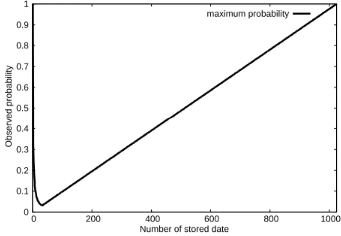
Then, how is the case where l 6= N. In this case, the

maximum probability is computed by solving dPw(t)/dt=

0. Fig.4 shows the results which arePw(t)6= 1 except for N =l andPw(t)≤0.5 for l < N/2.

B. Improved search algorithm in analog time

The state ψa(t1) of memorized data after t1 step and

the state ψb(t1) of non-memorized data after t1 step are

represented as follows:

ψa(t1) =

1

√

lcos

√

l Nt1+i

1

√

N sin

√

l

Nt1 (44)

ψb(t1) = i

1

√

N sin

√

l

Nt1 (45)

When t1 = (π/2) √

N/l, it holds ψa(t1) = ψb(t1).

Therefore, the states except for marked data at the step t1

0 0.1 0.2 0.3 0.4 0.5 0.6 0.7 0.8 0.9 1

0 200 400 600 800 1000

Observed probability

Number of stored date

maximum probability

Fig. 4. Maximum probability for the number of memorized data

are identical, so the method 1 is possible to apply at the time t=t1. The use of the method 1 for the time intervalt2leads

to the following probability:

ψw(t2+t1) =

i

√

N [(N−m)αm+ (m−1)βm+δm]

= i√1

N cos

√

m Nt2−

1

√

msin

√

m Nt2(46)

Pa(t2+t1) = 1

N cos

2 √

m Nt2+

1 msin

2 √

m

Nt2 (47)

By taking t2= (π/2)

√

N/m, it holds Pa(t1+t2) = 1/m.

The method is called the proposed method 2 in analog time. Fig.5 shows the numerical example the comparison between

method 1 and proposed method 2 forN= 1024, m= 1, l=

512.

0 0.1 0.2 0.3 0.4 0.5 0.6 0.7 0.8 0.9 1

0 20 40 60 80 100

Probability

time

method_1 The proposed method_2

Fig. 5. The comparison between the method 1 and the proposed method 2

C. The application to Grover search algorithm of the pro-posed methods

1. Initial state|ψi

2. RepeatT1 times

3. |ψi=I_ρ|ψi

4. |ψi=G_|ψi

5. RepeatTg times

6. |ψi=I_τ|ψi

7. |ψi=G_|ψi

8. Observe the system

Fig. 6. The algorithm of the proposed method 3

timeT1 as the same method used in the section B.

ψa(T1) =

1

√

lcosω1T1 (48)

ψb(T1) = −

1

√

N−lsinω1T1, (49)

where

ω1= arccos (

N−2l N

)

. (50)

Therefore, we can find the time when ψa(T1) = ψb(T1)as

follows:

T1= CI 

  

π−arctan

(_√

N−l l

)

arccos(_N−2l N

) 

  

, (51)

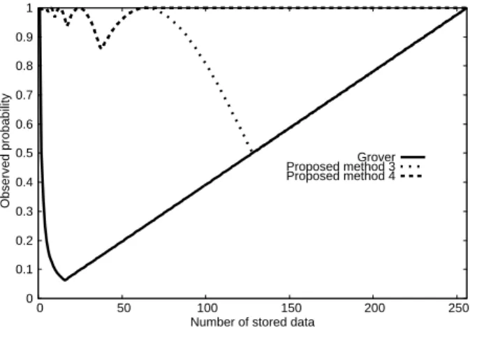
whereCI(x) means rounding of x. Fig.7 shows the result

0 0.1 0.2 0.3 0.4 0.5 0.6 0.7 0.8 0.9 1

0 50 100 150 200 250

Observed probability

Number of stored data

Grover Proposed method 3 Proposed method 4

Fig. 7. The comparison among the proposed algorithms

of numerical simulation for N = 256.

Example 2:

Let n = 4and N = 16. Let |2i,|6i,|11i,|12i be stored data.

|ψi= 1

2(0,0,1,0,0,0,1,0,0,0,0,1,1,0,0,0) t

(52)

The suffix t means the transpose of the vector The following reult is obtained by applyingI_{ρ and}G_{to the initial state of}

the Eq.52.

|ψi= 1

4(−1,−1,1,−1,−1,−1,1,−1,−1,−1,−1,1, 1,−1,−1,−1)t (53)

As T1 = 2, Iρ and G to the Eq.53 are iterated one more

time. As a result, the following state is obtained:

|ψi=1

4(−1,−1,−1,−1,−1,−1,−1,−1,−1,

−1,−1,−1,−1,−1,−1,−1)t ₍₅₄₎

Further, iterating the steps 5 to 8 of the proposed method 3 to the Eq.54, the desired data is obtained with the probability 0.96.

Next, supposing that the stored data are

|0i,|2i,|3i,|6i,|7i,|10i,|11i,|12ias follows:

|ψi= 1

2√2(1,0,1,1,0,0,1,1,0,0,1,1,1,0,0,0) t ₍₅₅₎

When the steps 2 to 4 of the proposed method 3 are iterated for the Eq.55, the following state is obtained:

|ψi=− 1

2√2(1,0,1,1,0,0,1,1,0,0,1,1,1,0,0,0) t ₍₅₆₎

Then, the desired data is obtained with the probability 0.5 after applying the steps 5 to 8. It shows that the proposed method 3 does not always give a good result.

As shown in Fig.7. we can not always get the maximum

result, because the maximum value ofT1 is real number in

analog model. Therefore, in order to improve the result we can introduce the phase rotation[8]. These are represented as the following unitary matrixes:

W ₌ I_−(1−e−iα₎

l

∑

k=1

|ρkihρk| (57)

V _{= (1−e}iβ_{)|sihs|+ e}iβI ₍₅₈₎

1. Initial state |ψi

2. RepeatT2 times

3. |ψi=W_|ψi

4. _|ψi=V_|ψi

5. RepeatTg times

6. |ψi=I_τ|ψi

7. |ψi=G_|ψi

8. Observe the system

Fig. 8. The algorithm for the proposed method 4

The method is called the proposed method 4 The Fig.8 shows the algorithm for the proposed method 4. MatrixesI_ρ

andG _{used before are the special case forα =β =π of}

W _andV_{, respectively. Let us compute the timeT2. Let us}

consider the case ofT2= 2. Then, as the imaginary parts of

ψa(2) andψb(2) are agree, we will find the condition that

the real parts of ψa(2) andψb(2) are agree. The following

relation is satisfied with the condition:

α= arccos

(

−N_2l−2l )

(59)

wherel≥(1/4)N

Fig.7 shows the results of Grover and two proposed algorithms.

Example 3:

Let n = 4 and N = 16. Let the initial state be defined

TABLE I

ASUMMARY OF THE PROPOSED METHODS.

Analog model Digital model Schroedinger Method 1 Grover algorithm

equation Proposed method 2 Proposed method 3 Proposed method 4

As T2 = 2, the steps 3 to 4 of the proposed method 4 are

iterated two times. Then, the following state is obtained:

|ψi= 1

4√2(−1 +i,−1 +i,−1 +i,−1 +i,

−1 +i,−1 +i,−1 +i,−1 +i−1 +i,−1 +i,

−1 +i,−1 +i,−1 +i,−1 +i,−1 +i,−1 +i)t ₍₆₀₎

Grover algorithm shows good performance only in the case

ofN =l. The proposed method 3 shows better performance

compared with Grover algorithm, but does not always show good performance in the case ofN 6=l.

The proposed algorithm 4 shows best performance of three algorithms in digital model.

V. CONCLUSIONS AND FUTURE WORK

The result in this paper is summarized in Table I. The method 1 and the proposed method 2 are obtained by solving the schrodinger equation. The method 1 and the proposed method 2 in analog time lead to Grover algorithm and the proposed method 3 in digital time. The proposed method 2 in analog time gives the optimum solution, but the proposed method 3 in digital method 3 does not give the optimum solution, because the optimum time is real number. Therefore, we propose the method 4 and show that it gives the optimum solution. As the future work, we will consider the relation between the proposed method 2 and 4.

REFERENCES

[1] P. Shor, “Polynomial-Time Algorithms for Prime Factorization and Discrete Logarithms on a Quantum Computer”, SIAM Journal of Computing, vol.26, no.5, pp.1484-1509, 1997.

[2] L. Grover, “A Fast Quantum Mechanical Algorithm for Database Search”, Proc. of 28th ACM Symp. on Theory of Computing, pp.212-219, 1996.

[3] D. Ventura and T. Martinez, “Quantum Associative Memory”, Informa-tion Science, vol.124, pp.273-296, 2000.

[4] D. Biron, O. Biham, E. Biham, M. Grassl and D.A. Lidar, “Generalized Grover Search Algorithm for Arbitrary Initial Amplitude Distribution”, Lecture Notes In Computer Science, Vol.1509, pp.140-147, 1998. [5] D. Ventura and T. Martinez, “Initializing the Amplitude Distri- bution

of A Quantum State”, Foundations of Physics Letters, Vol.12, No.6, pp.547-559, 1999.

[6] K. Arima, H. Miyajima, N.Shigei and M. Maeda, “Some Properties of Quantum Data Search Algorithms”, The 23rd Int. Technical Conf. on Circuits/Systems, Computers and Commu- nications, no.P1-42, pp.1169-1172, 2008.

[7] K. Arima, N. Shigei, H. Miyajima, “A Proposal of a Quantum Search Algorithm”, Fourth International Conference on Computer Sciences and Convergence Information Technology, pp.1559-1564, 2009.

[8] P. Li and K. Song “Adaptive Phase Matching in Grover’s Algorithm”, Journal of Quantum information Science, Vol.1, No.2, pp.43-49, 2011. [9] K. Akiba, T. Miyadera and M. Ohya, “Search by Quantum Walk on the Complete Graph”, Technical Report of IEICE, IT2004-17(2004-7), pp.53-58.