www.biogeosciences.net/10/7463/2013/ doi:10.5194/bg-10-7463-2013
© Author(s) 2013. CC Attribution 3.0 License.
Biogeosciences
Foraminiferal survival after long-term in situ experimentally
induced anoxia
D. Langlet1, E. Geslin1, C. Baal2, E. Metzger1, F. Lejzerowicz3, B. Riedel4, M. Zuschin2, J. Pawlowski3, M. Stachowitsch4, and F. J. Jorissen1
1Université d’Angers, UMR6112 CNRS LPG-BIAF – Bio-Indicateurs Actuels et Fossiles, 2 Boulevard Lavoisier, 49045
Angers Cedex, France
2University of Vienna, Department of Palaeontology, Althanstrasse 14, 1090 Vienna, Austria 3University of Geneva, Department of Genetics and Evolution, CH 1211 Genève 4, Switzerland
4University of Vienna, Department of Limnology and Oceanography, Althanstrasse 14, 1090 Vienna, Austria
Correspondence to:D. Langlet (dewi.langlet@univ-angers.fr)
Received: 19 April 2013 – Published in Biogeosciences Discuss.: 10 June 2013
Revised: 4 October 2013 – Accepted: 21 October 2013 – Published: 21 November 2013
Abstract.Anoxia was successfully induced in four benthic chambers installed at 24 m depth on the northern Adriatic seafloor from 9 days to 10 months. To accurately determine whether benthic foraminifera can survive experimentally in-duced prolonged anoxia, the CellTracker™ Green method
was applied and calcareous and agglutinated foraminifera were analyzed. Numerous individuals were found living at all sampling times and at all sampling depths (to 5 cm), sup-ported by a ribosomal RNA analysis that revealed that certain benthic foraminifera were active after 10 months of anoxia. The results show that benthic foraminifera can survive up to 10 months of anoxia with co-occurring hydrogen sulfides. However, foraminiferal standing stocks decrease with sam-pling time in an irregular manner. A large difference in stand-ing stock between two cores sampled under initial condi-tions indicates the presence of a large spatial heterogeneity of the foraminiferal faunas. An unexpected increase in standing stocks after one month is tentatively interpreted as a reaction to increased food availability due to the massive mortality of infaunal macrofaunal organisms. After this, standing stocks decrease again in cores sampled after 2 months of anoxia to then attain a minimum in the cores sampled after 10 months. We speculate that the trend of overall decrease of standing stocks is not due to the adverse effects of anoxia and hy-drogen sulfides but rather due to a continuous diminution of labile organic matter.
1 Introduction
Over the last decade, numerous marine environments have been affected by hypoxia (Diaz and Rosenberg, 2008). The increase in the frequency of occurrence of hypoxia and the spatial distribution of such oxygen-depleted areas are as-sumed to be linked to eutrophication and climate change (Stramma et al., 2008; Rabalais et al., 2010). Hypoxia can dramatically affect pelagic and benthic biodiversity (Levin, 2003; Gooday et al., 2009; Stramma et al., 2010). The mech-anisms leading to low-oxygen conditions differ between the open ocean and coastal enclosed basins. In many oceanic upwelling areas, hypoxia is permanent and the dissolved oxygen concentration remains below 0.5 mL L−1 (20 µM;
Helly and Levin, 2004; Middelburg and Levin, 2009). Hy-poxia is caused by a combination of high pelagic produc-tivity and slow renewal of oxygen in the water column. In most semi-enclosed coastal areas, hypoxia is related to con-tinental inputs (of nutrients and organic matter) and seasonal water-column stratification. Pelagic production is a response to natural and/or anthropogenic nutrient input, and hypoxia is mainly caused by benthic oxygen consumption. In such coastal environments hypoxia appears seasonally.
extreme cases, when the seafloor becomes anoxic, organic matter degradation continues via anaerobic metabolic pathways, eventually leading to sulfate reduction near the sediment–water interface (Middelburg and Levin, 2009). In such conditions toxic hydrogen sulfide may diffuse into the bottom water.
Various terminologies have been proposed to describe the intensity of hypoxia, mainly based on the effect of oxygen concentration on marine biota (reviewed in Hofmann et al., 2011 and Altenbach et al., 2012). For the purpose of the present study we will use only three terms defined as fol-lows (Tyson and Pearson, 1991; Bernhard and Sen Gupta, 1999; Middelburg and Levin, 2009): (1) oxic – the measured oxygen concentration above 1.5 mL L−1(>63 µM); (2)
hy-poxic – concentration below 1.5 mL L−1(<63 µM), which
is the threshold at which an impact has been recorded on coastal metazoan biota; and (3) anoxic – no detectable dis-solved oxygen present.
In the past, several field and laboratory studies have been conducted to better understand the response of benthic fau-nas to hypoxia (i.e., to low oxygen concentration and its co-occurring processes such as high organic matter availability and increased hydrogen sulfide concentration) in coastal en-vironments. These studies demonstrate that for macrofauna (invertebrates larger than 1 mm) the first responses to low oxygenation are usually behavioral or physiological changes (e.g., body extension, shallowing of burial depth, emergence from the sediment; see Levin et al. (2009) for a review), and the organisms exhibit a high mortality rate after only two to seven days of anoxia (Riedel et al., 2008; Stachow-itsch et al., 2012). Within the meiofauna (invertebrates mea-suring 45 µm to 1 mm), copepods are among the taxa most sensitive to anoxia (Moodley et al., 1997; Diaz and Rosen-berg, 2008), whereas several nematode species can survive up to 60 days of anoxia (Wieser and Kanwisher, 1961). Ben-thic foraminifera appear to be more tolerant to anoxia than most meiofaunal metazoans (Josefson and Widbom, 1988; Moodley et al., 1997; Levin et al., 2009).
In field studies, the foraminiferal density tend to de-crease during anoxic and/or hypoxic events (e.g., Jorissen et al., 1992; Duijnstee et al., 2004) and infaunal taxa mi-grate upward in hypoxic conditions (Alve and Bernhard, 1995; Duijnstee et al., 2003). In the diatomaceous mud belt off Namibia,Virgulinella fragilisappear to be the only foraminiferal species that can survive anoxic and sulfidic conditions (Leiter and Altenbach, 2010). Laboratory stud-ies show that foraminiferal assemblages can survive up to 78 days of anoxia (Moodley et al., 1997). Conversely, benthic foraminiferal densities respond positively to increased input of fresh organic matter if it is not accompanied by oxygen de-pletion (Heinz et al., 2001; Ernst and van der Zwaan, 2004; Ernst et al., 2005; Nomaki et al., 2005). Some evidence sug-gests that an exposure to hydrogen sulfide for up to 21 days does not significantly affect foraminiferal density, and that
after 66 days of exposure, some individuals were still found alive (Moodley et al., 1998).
Most previous studies were based on the analysis of foraminiferal assemblages stained by rose bengal. Rose ben-gal is a bulk stain that adheres to the proteins present in the protoplasm (Walton, 1952; Bernhard, 2000). How-ever, protoplasm may be preserved in the foraminiferal shell several days to weeks after the death of the organ-ism in well-oxygenated conditions (Boltovskoy and Lena, 1970; Bernhard, 1988; Murray and Bowser, 2000) and up to three months in anoxia (Hannah and Rogerson, 1997), leading to the staining of dead organisms. The expectation is that protoplasm degradation is especially slow in anoxic conditions (Burdige, 2006; Glud, 2008). Consequently, us-ing rose bengal can lead to substantial overestimation of the living foraminiferal standing stocks, and probably does not reliably reflect the living faunas in low-oxygen settings. Al-though rose bengal staining may yield a rapid overview of living faunas in distributional studies, it is unsatisfactory for studies with a high temporal resolution, where the time be-tween successive samplings may be shorter than the time needed for degradation of the foraminiferal protoplasm. Sev-eral techniques have recently been developed to more accu-rately identify the vitality of benthic foraminifera (reviewed in Bernhard, 2000). As noted above, proteins can still be present after the organism has died and all energetic and enzymatic activities have stopped. These activities are the basis for more accurate foraminiferal vitality discrimination techniques. For instance, based on an adenosine triphosphate (ATP) concentration, an absence of living individuals was de-termined in the Santa Barbara Basin after a 10-month anoxic period (Bernhard and Reimers, 1991). A laboratory exper-iment using the ATP concentration method determined, in four species from a shallow site (45 m) in Drammensfjord (Norway), that all these species survived up to three weeks of anoxia. Three species, however, showed a lower ATP con-centration in anoxic conditions (Bernhard and Alve, 1996). A recent laboratory experiment (Piña-Ochoa et al., 2010b) us-ing the enzymatic activity sensor fluorescein diacetate (FDA; Bernhard et al., 1995) showed that the deep infaunal species
Globobulimina turgidacan survive anoxia (with presence of nitrate) for up to 84 days (with a survival rate of 46 %). A subsequent study, using the same method, demonstrated that the individuals do not migrate vertically during anoxia (Koho et al., 2011). CellTracker™ Green (CTG; Bernhard et al.,
2006), another enzymatic activity probe, has been used to determine that Adriatic Sea foraminiferal assemblages can survive up to 69 days of hypoxia and that their vertical migra-tional behavior is largely linked to the labile organic matter availability (Pucci et al., 2009). Finally, it has been shown re-cently that the active status of foraminifera can be confirmed by sequencing a taxonomic marker extracted from the sedi-ment metatranscriptome (Lejzerowicz et al., 2013).
for prolonged periods, in most cases without a clear de-crease in population density. Many of these studies, however, are based on the problematic rose bengal staining method, which may substantially overestimate the number of living individuals or even indicate “living” faunas where none are present, especially in anoxic conditions. This calls for testing the resistance of shallow-water foraminifera to anoxia with a more reliable vitality determination technique. Addition-ally, until now the foraminiferal response to strong hypoxia and/or anoxia has mainly been assessed by laboratory exper-iments and by ecological field studies lasting up to 3 months, but never (to our knowledge) by an in situ experiment over 10 months. The current paper applies such a long-term in situ experimental approach to document the foraminiferal re-sponse to anoxia, using the CTG technique. Our experimen-tal setup was designed to address several complementary as-pects of the benthic ecosystem:
1. In order to ensure long-term anoxia (up to ∼10
months), several benthic chambers were positioned on the sea floor for different periods of time. After closure of the chambers, the respiration of the benthic organ-isms rapidly consumed all available oxygen, leading to anoxia. In order to quantify these processes, the chem-ical characteristics of the sediment and the overlying waters were monitored (Koron et al., 2013; Metzger et al., 2013).
2. An in situ experimental approach has the advantage of considerably reducing “laboratory effects” due to dif-ferences between experimental and natural conditions, as well as of reducing the natural temporal variabil-ity (in temperature, salinvariabil-ity, water transparency, food availability, etc.) that can affect faunas in field studies. 3. Our experimental setup allows us to apply the same method on different faunal elements. It has been suc-cessfully used to study the effect of anoxia on macro-fauna (Riedel et al., 2008, 2012, 2013; Stachowitsch et al., 2012; Blasnig et al., 2013) and on different meio-faunal groups such as copepods, nematodes (De Troch et al., 2013; Grego et al., 2013) and foraminifera (this study and Langlet et al., 2013).
Our study was conducted in the northern Adriatic Sea, which is a typical coastal area impacted by seasonal hy-poxia/anoxia. It combines many aspects commonly associ-ated with low-oxygenation events: a semi-enclosed, shal-low (<50 m) basin with a fine-grained substrate, a high riverine input, high productivity (leading to “marine snow” events), and long water residence times in summer/autumn (Ott, 1992). Several studies have reported the occurrence of bottom-water hypoxia and anoxia here (e.g., Giani et al., 2012), with an increasing frequency from the 1970s to the mid-1990s. It appears that the frequency of marked hypoxia has decreased since the mid-1990s (Giani et al., 2012), likely
Table 1.Deployment and sampling dates as well as duration of the experimental period for the cores representing in situ conditions (“Normoxia”) and the various periods of anoxia in the four different benthic chambers
Sample ID Chamber Core sampling Incubation
deployment day day duration
Normoxia – 3 Aug 2010 0 days
9 days 2 Aug 2010 11 Aug 2010 9 days 1 month 27 Jul 2010 25 Aug 2010 29 days 2 months 27 Jul 2010 23 Sep 2010 58 days 10 months 24 Sep 2010 5 Aug 2011 315 days
due to a reduction of anthropogenic nutrient supplies and a reduced riverine nutrient input into the northern Adriatic Sea. In this context, we investigate the responses of the foraminiferal faunas to experimentally induced anoxia in benthic chambers. The present paper focuses on the foraminiferal survival and density response to long-term anoxia. Our main question was whether benthic foraminifera could survive 10 months of anoxia. In the case of a positive answer, our goal was to determine how the density varies as a function of the duration of anoxia. Finally, we studied the variation of density in the upper 5 cm of the sediment in order to identify potential vertical migration of the foraminiferal faunas in response to experimental conditions. The response of individual species to anoxia is treated in a second paper (Langlet et al., 2013).
2 Material and methods
2.1 Experimental setup and sampling
The experiment was conducted in the Gulf of Trieste (north-ern Adriatic Sea) near the oceanographic buoy of the Ma-rine Biology Station Piran (45◦32.90′N, 13◦33.00′E) at 24 m
depth on a poorly sorted silty sandy bottom. The experimen-tal setup has been adapted from an earlier experiment con-ducted by Stachowitsch et al. (2007) and Riedel et al. (2008). Both experiments used the Experimental Anoxia Generating Unit (EAGU), which is a 0.125 m3 fully equipped benthic
chamber (a cube with all sides 0.5 m long) that enables exper-imentally inducing and documenting local-scale anoxia (see Stachowitsch et al., 2007).
(termed “normoxia”) were sampled at the start of the exper-iment. In order to standardize the terminology for all arti-cles of the present Biogeosciences Special Issue, the differ-ent sampling times (also named in the presdiffer-ent paper “sample ID” for “sample identification”) have been termed “9 days”, “1 month”, “2 months” and “10 months”. The exact dura-tion (in days) of each of the experiments is given in Table 1. The first chamber, fully equipped with the EAGU analytical devices, documented the onset of anoxia during a 9-day pe-riod. The other three chambers were used to study the devel-opment of the meiofauna after∼1 month,∼2 months and
about 10 months of anoxia, respectively. Foraminifera, cope-pods and nematodes were analyzed for the same cores. Sed-iment cores were taken by scuba divers using a Plexiglas™
corer with a 4.6 cm inner diameter (16.6 cm2 surface area).
Two replicate cores were taken in each of the benthic cham-bers at each sampling time.
2.2 Meiofaunal analysis
To identify whether the collected meiofaunal organisms were alive, we used CellTracker™ Green CMFDA (5-chloromethylfluorescein diacetate; Molecular Probes, Life Technologies; heretofore called “CTG”). When living cells are incubated in CTG, this nonfluorescent probe passes through the cellular membrane and reaches the cytoplasm, where hydrolysis with nonspecific esterase produces a fluo-rogenic compound. This fluofluo-rogenic compound does not leak out of the cell after fixation and can thus enable identifying the individuals exhibiting enzymatic activity when sampled (Bernhard et al., 2006).
For meiofaunal analyses, entire sediment cores were sliced every half centimeter from 0 to 2 cm and every centimeter be-tween 2 and 5 cm. Within one hour after retrieval, sediments were stored in 100 cm3 bottles, which were filled with sea water and CTG-DMSO (dimethyl sulfoxide) at a final CTG concentration of 1 µM (Bernhard et al., 2006; Pucci et al., 2009). Samples were gently shaken and immediately placed in a cold room at in situ temperature, where they remained for at least 10 h in order to obtain the hydrolysis of the CTG probe. After this reaction period, samples were fixed in 4 % formaldehyde buffered with sodium tetraborate. The samples were further stored at room temperature.
Samples were then centrifuged to separate the soft meio-fauna (i.e., copepods, nematodes; results presented in De Troch et al., 2013 and Grego et al., 2013) from the sed-iment and the “hard-shelled” meiofauna (i.e., foraminifera – the present article and Langlet et al. (2013)). Centrifuga-tion has two main advantages: first it permits working on the same sample for both copepods/nematodes and foraminifera. These two groups are easily separated because of their dif-ferent densities; foraminifera are heavier because of their agglutinated or calcareous test. Secondly, it simplifies the foraminiferal analysis because all the soft organisms, which show a stronger fluorescence than foraminifera (the test tends
to diminish the observed intensity of the fluorescence), have been removed.
Prior to centrifugation, samples were first sieved over a 38 µm mesh to remove small sediment particles and formaldehyde. We then added a Levasil density medium and distilled water to achieve a density of about 1.17 g cm−3,
and finally added about 10 g of kaolin powder to promote the sedimentation of the heavier particles (McIntyre and Warwick, 1984; Burgess, 2001). Next, we centrifuged for 10 min at 3000 rpm at ambient room temperature. After this, the supernatant (composed of soft meiofauna) and the de-posit (composed of the hard-shelled meiofauna and sedi-ment) were separately sieved over a 38 µm mesh to remove the kaolin and the Levasil medium. The two separated sam-ples were stored in a borax-buffered formaldehyde solution until further analysis.
The present study analyzes only the samples contain-ing the hard-shelled meiofauna (soft-walled foraminiferal taxa are excluded). Therefore, this contribution only con-siders calcareous and agglutinated foraminifera. These sam-ples were subsequently sieved over 315, 150, 125 and 63 µm meshes.
A major asset of the present study is that we also analyzed all of the>63 µm size fractions of the benthic foraminifera, and we systematically studied the complete sample without splitting. Many studies fail to analyze the smaller size frac-tions (63–125 or 63–150 µm) because it is extremely time consuming. The smaller size fraction, however, may contain abundant living individuals and can provide important infor-mation about small opportunistic species and about potential reproduction during the experiment.
For the 63–125 µm fractions it was necessary to use a concentration method for the foraminifera to prevent split-ting the sediment (leading to statistical problems) and/or un-realistic working times. Thus, all foraminiferal samples of the fractions 63–125 µm were washed to remove the borax-buffered formaldehyde solution and then dried in a compart-ment dryer (Memmert GmbH+Co.KG) at 30–40◦C. The
foraminiferal tests were then separated by treating the sedi-ment with tetrachloride under a laboratory fume (Hoheneg-ger et al., 1989; Murray, 2006). The tetrachloride was care-fully decanted and the floating foraminifera were collected on paper filters, quickly dried and then stored in small glass vials.
Foraminiferal counts were performed in all fractions
>63 µm using an epifluorescence stereomicroscope
2.3 Ribosomal RNA analysis
Total RNA was extracted from ca. 0.5 g of sediment from the top centimeter of one single core collected in the “10 months” anoxia chamber using the PowerSoil Total RNA Isolation Kit according to the manufacturer’s instructions (MoBio). For each sample, a 30 µL aliquot of RNA extract was purified from co-extracted DNA by incubating 2 units of TURBO DNase enzyme (Ambion) in the presence of 3 µL of its 10X buffer for 25 min at 37◦C. An additional
incuba-tion with another 2 units of DNase was conducted in order to guarantee the total digestion of small DNA fragments. Then, the digestion was stopped by adding 5 µL of DNase Inacti-vation Reagent (Ambion) and incubating 2 min at ambient temperature. After centrifugation for 90 s at 10 000 g, the su-pernatant was collected and the absence of double-stranded DNA was confirmed by PCR amplification. This control PCR reaction was conducted on 1 µL of DNase-treated RNA in a total volume of 15 µL containing 1 units of Taq Poly-merase (Roche), 1X of buffer solution (Roche), 0.2 µM of each primer s14F3 (5′-ACGCAMGTGTGAAACTTG-3′)
and s17 (5′-CGGTCACGTTCGTTGC-3′), and 0.2 mM of
each dNTP. The reaction consisted of a pre-incubation at 94◦C for 90 s, followed by 25 cycles of 94◦C for 1 min,
50◦C for 1 min and 72◦C for 45 s, 10 cycles of 94◦C for
30 s, 50◦C for 30 s and 72◦C for 45 s, and a final incubation
at 72◦C for 120 s. The amplification results are presented
in the Supplement, Fig. 1. The complementary strands of ca. 150 ng of RNA (i.e., cDNA) were synthesized for each sample using the SuperScriptIII®Reverse Transcriptase
(In-vitrogen). Present in a volume of 11 µL of RNA were pre-mixed 1 µL of 10 mM dNTPs and 1 µL containing 250 ng of random primers (Promega). After an incubation for 5 min at 65◦C and then for 2 min on ice, 4 µL of 5X RT buffer
(In-vitrogen), 1 µL of 100 mM dithiothreitol (DTT) and 200 U of SuperScriptIII®Reverse Transcriptase (Invitrogen) were added to the pre-mix. The reverse transcription was con-ducted for 5 min at 25◦C, followed by 50 min at 55◦C and
15 min at 15◦C. A control with no RNA was included and
amplified as described in the next section in order to moni-tor the occurrence of contamination during the cDNA syn-thesis. The resulting cDNA were used as template to am-plify, clone and sequence the foraminifera-specific hyper-variable region 37f of the small subunit of the ribosomal RNA gene (SSU rDNA) as in Pawlowski et al. (2011) but us-ing the above primers and no re-amplification. The resultus-ing sequences were filtered for chimeras using UChime and each sequence assigned to a foraminiferal species or genus based on the taxonomically informative 37f hypervariable region (Pawlowski and Lecroq, 2010). Briefly, each of the 61 se-quences was aligned to 1003 curated reference sese-quences of the corresponding 37f hypervariable foraminiferal region us-ing the Needleman–Wunsch algorithm and the best match(s) under a threshold of 20 % dissimilarity was retained for as-signment. In those cases where more than one reference
se-quence matched the environmental sese-quence at the lowest distance, the environmental sequence was assigned to the deepest consensus of taxonomy without conflict of these ref-erence sequences, as in Lecroq et al. (2011). Pairwise global alignments between all assigned sequences were also used to form clusters or operational taxonomic units (OTUs) using the software mothur v1.28.0 (Schloss et al., 2009). A thresh-old of 4 % sequence dissimilarity was chosen as no further sequence clustered until a distance of 16 %. The resulting OTUs were assigned according to the consensus of the as-signments for individual sequences. The analyzed sequences were submitted to GenBank under the accession numbers KF647255 to KF647315.
2.4 Data analysis
After the discrimination of the living individuals, they were counted and expressed as standing stock (number of living individuals per core in the 0–0.5 or in the 0–5 cm depth in-terval normalized for a 10 cm2 surface area) and as density
(number of living individuals per depth interval normalized for a 10 cm3sediment volume).
Three statistical procedures were used to identify the effect of several parameters on the foraminiferal standing stocks or density. All the procedures are linear models (Chambers and Hastie, 1992) in which the dependent variable (the re-sponse variable) is the log-transformed foraminiferal density or standing stock. The log-transformation ensures that the de-pendent variable shows a Gaussian distribution.
To be able to determine significant differences in the foraminiferal standing stocks between sampling times, two models test the effect of the sample ID (i.e., a qualitative ex-pression of the sampling time) on standing stocks over two depths intervals. The first model tests the sample ID effect in the whole core (0–5 cm; Table 2, Model 1), the second only for the shallowest depth interval (0–0.5 cm; Table 2, Model 2).
Table 2.Summary of the variables used in each of the three linear models, describing the name of the variable, its type (dependent or inde-pendent), its unit, nature (quantitative or qualitative) and the used transformation. For the quantitative variables the minimum and maximum values of the nontransformed data are presented in brackets, whereas for the qualitative variables the different categories are presented in brackets.
Name Variable Type Unit Variable nature (values) Transformation
Model 1: Analysis of variance
Standing Stock (0–5 cm) Dependent Ind./10 cm2 Quantitative (min=533; max=1979) log (1+Standing Stock) Sample ID Independent – Qualitative (“normoxia”, “9 days”,
“1 month”, “2 months” and “10 months”)
–
Model 2: Analysis of variance
Standing Stock (0–0.5 cm) Dependent Ind./10 cm2 Quantitative (min=115; max=529) log (1+Standing Stock) Sample ID Independent – Qualitative (“normoxia”, “9 days”,
“1 month”, “2 months” and “10 months”)
–
Model 3: Analysis of covariance
Standing Stock Dependent Ind./10 cm2 Quantitative (min=115; max=1979) log (1+Standing Stock)
Depth Interval Independent – Qualitative (“0–5 cm” and “0–0.5 cm”) –
Time Independent days Quantitative (min=0; max=315) log (5+Time)
Depth Interval×Time Independent – Interaction –
Model 4: Analysis of covariance
Density Dependent Ind./10 cm3 Quantitative (min=46; max=1059) log (1+Density)
Depth Independent cm Quantitative (min=0.25; max=4.5) log (1+Depth)
Depth2 Independent cm Quantitative (min=0.25; max=4.5) (log (1+Depth))2 Sample ID Independent – Qualitative (“normoxia”, “9 days”,
“1 month”, “2 months” and “10 months”)
–
Depth×Depth2 Independent – Interaction –
Depth×Sample ID Independent – Interaction –
Depth2×Sample ID Independent – Interaction –
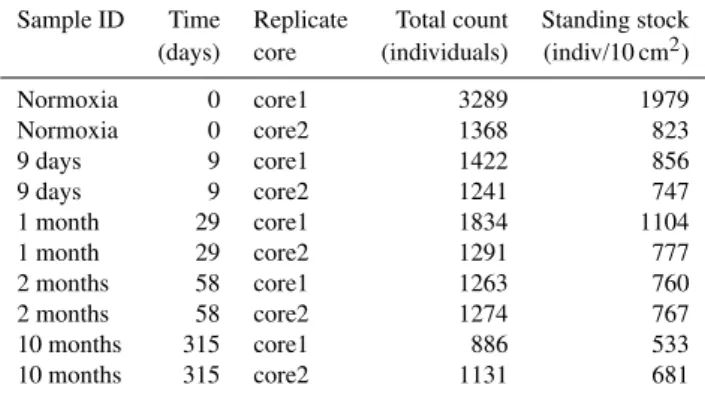
Table 3. Total counts and standing stocks at every sampling time for every replicate core.
Sample ID Time Replicate Total count Standing stock (days) core (individuals) (indiv/10 cm2)
Normoxia 0 core1 3289 1979
Normoxia 0 core2 1368 823
9 days 9 core1 1422 856
9 days 9 core2 1241 747
1 month 29 core1 1834 1104
1 month 29 core2 1291 777
2 months 58 core1 1263 760
2 months 58 core2 1274 767
10 months 315 core1 886 533
10 months 315 core2 1131 681
Finally, to quantify the effect of the anoxia and of sediment depth on the foraminiferal density, we designed an analysis of covariance linear model. The first computed model (Ta-ble 2, Model 4) tests the effect of the sample ID, the sediment depth (i.e., here a quantitative expression of the depth inter-val, the value used being the midpoint of the depth intervals) and their first-order interaction with foraminiferal density. Note that to increase the quality of the fit, sediment depth has been log-transformed and has been introduced with a
polynomial component (the log-transformed depth has been squared). The depth times squared depth interaction and the squared depth times sample ID interaction have also been added to the model.
Table 4 shows only the tested variables that have a signifi-cant effect. Table 2 in the Supplement shows how each of the variables affects the dependent variable.
3 Results
3.1 Foraminiferal survival under various experimental conditions
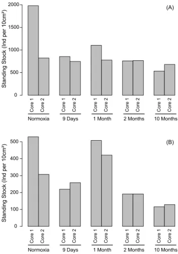
Living benthic foraminifera (i.e., positively labeled with CTG) were present from the beginning of the experiment to the end, after about 10 months of anoxia. Relatively large standing stocks were recorded from the surface down to 5 cm depth (Fig. 1, Table 3). In the 10 studied cores, the total number of individuals in the top 5 cm varied from
∼1980 individuals per 10 cm2in “normoxia” core 1 to∼530
Standing Stock (Ind per 10cm²)
0 500 1000 1500 2000
(A)
(B)
Standing Stock (Ind per 10cm²)
0 100 200 300 400 500
Normoxia 9 Days 1 Month 2 Months 10 Months
Core 1 Core 2 Core 1 Core 2 Core 1 Core 2 Core 1 Core 2 Core 1 Core 2
Normoxia 9 Days 1 Month 2 Months 10 Months
Core 1 Core 2 Core 1 Core 2 Core 1 Core 2 Core 1 Core 2 Core 1 Core 2
Fig. 1.Foraminiferal standing stocks in all sampled cores for the whole cores (0–5 cm, panelA) and for the 0–0.5 cm depth intervals (panelB).
Lagenammina atlantica, Hopkinsinella glabra, Bolivina pseudoplicata and Quinqueloculina stelligera were other conspicuous faunal elements. Census data are presented in the Supplement, Table 1; a more complete description and analysis of the faunal composition is presented in Langlet et al. (2013).
3.2 Density variation with time
Figure 1 shows that living benthic foraminifera (i.e., CTG-stained) were present at every sampling time. The standing stocks in the whole cores (0–5 cm depth interval; Fig. 1, Panel A) varied only slightly with incubation time. Although a clear maximum was found in “normoxia” core 1, no signif-icant differences existed between the pairs of replicate cores of the five sampling times (Table 4, Model 1). When only the 0–0.5 cm depth interval is considered, the highest standing stocks occurred in “normoxia” core 1 and very similar val-ues were found in both “1 month” cores, whereas the valval-ues were lowest (∼ 30 individuals per 10 cm3)in the two “10 months” cores.
5
Normoxia 9 Days 1 Month 2 Months 10 Months
10 20 50 100 200
0
500
1000
1500
2000
log (5+Time) (Days)
Standing Stock (Ind. per 10cm²)
●
●
●
●
● ●
●
●
●
● ●
0−5cm 0−0,5cm
Model 3
Fig. 2. Foraminiferal standing stocks plotted against deployment time. Open circles represent standing stock in the 0–5 cm depth interval, filled black circles correspond to the standing stock in 0–0.5 cm depth. Solid black lines represent the modeled stand-ing stocks plotted against time, for the two depth intervals, after Model 3. Note that incubation time is represented on a transformed log scale (5+time).
Model 2 (Table 4) was used to test whether the foraminiferal densities in the 0–0.5 cm depth interval (Fig. 3) were significantly different at different sampling times. The test shows that the standing stocks of the “normoxia” and the “1 month” cores are not significantly different, but both are significantly higher than the 0–0.5 cm densities of the “9 days” and “2 months” cores. The latter cores are not signifi-cantly different from each other (Table 4, Model 2 and Sup-plement Table 2). Finally, the standing stocks of the 0–0.5 cm layer of the “10 months” cores are significantly lower than those observed in all other cores (Table 4).
The analysis of covariance reveals that the total stand-ing stocks showed a significant exponential decrease both for the total cores (0–5 cm) and for the 0–0.5 cm level in function of log-transformed experimental time (Fig. 2; Ta-ble 4, Model 3). The density was significantly lower in the 0–0.5 cm depth interval than in the whole core (Table 4, Model 3), indicating that a significant part of the living fauna was present in deeper sediment levels.
The slopes of the regression curves between the 0–5 cm and 0–0.5 cm intervals were not significantly different (Ta-ble 4, Model 3). This means that the density decrease over time was not significantly different between the whole core (0–5 cm) and the topmost sediment (0–0.5 cm).
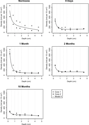
3.3 Density variation with sediment depth
● ● ● ● ● ● ● ● ● ● ● ● ● ● ● ● ● ● ● ● ● ● ● ● ● ● ● ● ● ● ● ● ● ● ●
0 1 2 3 4 5
0 200 400 600 800 1000 Normoxia Depth (cm)
Density (ind per 10 cm
3)
0 1 2 3 4 5
0 200 400 600 800 1000 9 Days Depth (cm)
Density (ind per 10 cm
3)
0 1 2 3 4 5
0 200 400 600 800 1000 1 Month Depth (cm)
Density (ind per 10 cm
3)
0 1 2 3 4 5
0 200 400 600 800 1000 2 Months Depth (cm)
Density (ind per 10 cm
3)
0 1 2 3 4 5
0 200 400 600 800 1000 10 Months Depth (cm)
Density (ind per 10 cm
3) ●
Core 1 Core 2 Model 4
Fig. 3.Foraminiferal density plotted against sediment depth for all sampled cores. Open circles represent the density in replicate core 1, filled black circles that in core 2. Solid black line represents the modeled density according to model 4.
expression of time) effect is significant (Table 4, Model 4). When the various depth levels are considered individually, the densities in the “10 months” cores were significantly lower than those of the other four pairs of replicate cores (Table 4, Model 4 and Supplement Table 2). Additionally, the slopes of the density decrease with depth were not sig-nificantly different except for the one observed for the “1 month” cores, which is significantly steeper, mainly due to the very high density in the topmost level and the very strong decrease in the 0.5–1 cm level.
3.4 Ribosomal RNA analysis
A total of 61 filtered foraminiferal SSU rDNA sequences were obtained from the metatranscriptomic sediment ex-tract of the “10 months” anoxic chamber. After clustering, 32 OTUs were obtained, that included 15 unassigned OTUs (Fig. 4a). The remaining OTU were assigned to the calcare-ous order Rotaliida (9 OTUs), the agglutinated Textulariida (2 OTUs) and to the soft-walled monothalamiids (6 OTUs).
Bolivina Bulimina Buliminella Stainforthia Cibicidoides Epistominella Cycloclypeus Planorbulina Eggerella Reophax Bowseria CladeBM Psammophaga Crithionina CladeY UNDET Rotaliida Textulariida Monothalamiids Undetermi ned
A
B
Fig. 4.Taxonomic composition of the foraminiferal ribosomal RNA OTUs (operational taxonomy units) clustered at 96 % sequence identity from the top centimeter of the sediment in the “10 months” chamber.(A)Relative proportions of the 32 OTUs identified to the order level or left unassigned after taxonomic assignment based on Needleman-Wunsch global alignments of the 37f hypervariable re-gion as in Lejzerowicz et al. (2013). (B) Relative proportion of
OTUs (inner circle) and sequences (outer circle) assigned to the genus level.
One OTU represented by one sequence perfectly matched the reference sequence of a specimen that was morphologically determined asEggerella scabra and collected in the same area (Fig. 4b).
4 Discussion
4.1 Pore water geochemistry and macrofaunal behavior during the experiment
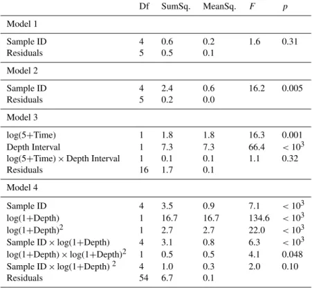
Table 4. Results of the models 1, 2, 3 and 4. For each model, the degrees of freedom (Df), the sum and mean of squares (SumSq. and MeanSq.), theF value (F) and itspvalue (p) are given for each variable. Thepvalues indicate whether the variable has a significant effect (p <0.05) or not (p >0.05).
Df SumSq. MeanSq. F p
Model 1
Sample ID 4 0.6 0.2 1.6 0.31
Residuals 5 0.5 0.1
Model 2
Sample ID 4 2.4 0.6 16.2 0.005
Residuals 5 0.2 0.0
Model 3
log(5+Time) 1 1.8 1.8 16.3 0.001
Depth Interval 1 7.3 7.3 66.4 <103
log(5+Time)×Depth Interval 1 0.1 0.1 1.1 0.32
Residuals 16 1.7 0.1
Model 4
Sample ID 4 3.5 0.9 7.1 <103
log(1+Depth) 1 16.7 16.7 134.6 <103
log(1+Depth)2 1 2.7 2.7 22.0 <103
Sample ID×log(1+Depth) 4 3.1 0.8 6.3 <103 log(1+Depth)×log(1+Depth)2 1 0.5 0.5 4.1 0.048
Sample ID×log(1+Depth)2 4 1.0 0.3 2.0 0.10
Residuals 54 6.7 0.1
was closed. The consumption rate was 950 nL cm−2h−1
(i.e., 0.0115 nmol cm−2s−1 or 9.93 mmol m−2day−1).
Mi-crosensor data show that hypoxia was reached after two to six days and anoxia after seven days. The overlying wa-ter remained anoxic until the end of the deployment (nine days). To estimate the contribution of the foraminiferal as-semblages to the oxic respiration in our benthic chambers, we compared the oxygen consumption rate with the to-tal foraminiferal respiration estimated using the power re-lation between foraminiferal biovolume and respiration rate (Geslin et al., 2011). The application of this relation, tak-ing into account the foraminiferal densities in the oxy-genated sediment layer (the 0–0.5 cm interval of the “nor-moxia” cores) in four distinct size classes (63–125, 125–150, 150–315 and>315 µm) yields a total foraminiferal respira-tion rate of 4.57 nL cm−2h−1. In comparison, the value is
950 nL cm−2h−1for total benthic respiration (Metzger et al.,
2013). Accordingly, foraminifera are responsible for about 0.5 % of the total benthic respiration in the chamber. These values are similar to those estimated for assemblages inhab-iting the Rhone prodelta (0.6 and 1.2 % at 37 and 60 m depth, respectively; Geslin et al., 2011; Goineau et al., 2011). Nev-ertheless, as these estimations are based on the standing stock of foraminifera larger than 63 µm, and thus neglect all the smaller individuals, these values probably underestimate the respiration rates of the whole foraminiferal community.
At the beginning of each experiment, 2 to 3 brittle stars (Ophiothrix quinquemaculata) were placed into each cham-ber, which otherwise contained no visible macroepifauna.
Ophiothrixshows typical behavioral reactions to decreasing
oxygen concentrations, such as arm tipping at the transition from normoxia to hypoxia, probably to raise the position of the respiratory organs in the water column (see Riedel et al., 2008, 2012, 2013). This macrofaunal behavior (includ-ing emerg(includ-ing infaunal species) was used as an additional in situ indicator for the onset of hypoxia in each chamber. The brittle stars and the other macrofaunal organisms died after 7 to 15 days of deployment. Shortly after the brittle stars died, the normally greyish-brown sediment turned black a few cen-timeters around the dead organisms. About 2 days later (i.e., after 9 to 17 days of deployment), the whole surface of the sediment in the chambers was completely black.
be progressive in the sediment column, the chemical com-position of the overlying waters shows a more complex pat-tern. The “1 month” probes showed a considerable increase of free sulfide hydrogen above the sediment–water interface. No such intensive sulfide production was observed in the “2 months” and “10 months” samples. This particular pattern caused an inverse sulfide gradient and consequently a down-ward sulfide flux into the sediment. In the “1 month” sample, sulfide was still detected 2 cm below the interface. These ob-servations have been interpreted to reflect the degradation of the dead macrofaunal remains concentrated at the sediment surface. Previous studies at the same site, using the same ex-perimental protocol, have shown that the macrofaunal organ-isms suffer massive mortality during the first week of anoxia (Riedel et al., 2008, 2012). The geochemical results (Met-zger et al., 2013) and especially the decrease in biogeochem-ical activity suggest that the abundant labile organic mat-ter resulting from macrofaunal mortality (the already present infaunal organisms and the introduced brittle stars) is con-sumed in the first month(s) of the experiment. Finally, the geochemical analyses also indicate that nitrates were present both in the overlying water and in the pore waters at all times, without any major changes in vertical distribution (Koron et al., 2013).
To summarize, the pore water chemistry indicates that the oxygen concentration decreased during the first days of the experiment. Anoxia was reached after 7 days, and was main-tained until the end of the experiment after 315 days. Sedi-ment geochemistry also suggests that a nonnegligible amount of fresh organic matter was added to the system due to the mortality of the macrofauna. This newly available labile or-ganic matter was consumed in the first month(s) of the ex-periment.
4.2 Methodological strategy of the study
The present study is original for combining an in situ experi-ment with the use of the very accurate CTG labeling method (instead of the traditional rose bengal staining method) and for the very long duration of the anoxia.
We believe our experimental approach to have three vantages compared to laboratory experiments. The first ad-vantage is that it circumvents undesirable laboratory effects, such as stress from transport and/or culture maintenance, re-production after incubation (e.g., Geslin et al., 2014; Ernst et al., 2006; Murray, 2006), and slightly differing environ-mental conditions (temperature, light, salinity, etc.). In com-parison to nonexperimental field studies, our experimental setup allowed us also to prolong the anoxic period and to avoid the effect of seasonal variation of food supplies. Con-versely, our closed setup blocked food supply from the out-side, and toxic components such as sulfides are not dispersed in the water column. Moreover, deployment by scuba divers to 24 m depth limits the available manpower and manipula-tion time precluding sampling every month and obtaining a
higher temporal resolution. Finally, our cores were taken a few decimeters from each other, potentially resulting in im-portant variation related to spatial patchiness, especially in the distribution of macrofaunal organisms and burrows, and the related biogeochemical processes. Laboratory studies can avoid the effects of patchiness by sieving and homogenizing the sediment, which could in turn affect the results pertaining to more sensitive species (Langezaal et al., 2004). Nonethe-less, we think that the advantages of our in situ approach out-weigh the disadvantages.
individuals. To do so, active (moving), nonactive (nonmov-ing) and clearly dead individuals were incubated in CTG. This calibration tests shows clear differences in the fluores-cence intensity and patterns. It has been previously evidenced that foraminiferal cytoplasm can be (partially) overtaken by bacteria and still positively stain with rose bengal (Bern-hard et al., 2010). Such a possibility cannot be entirely ex-cluded either with the CTG method, since living bacteria also react positively to CTG. In our material, for some speci-mens the fluorescence intensity was rather low, and appeared patchy and “milky”. We assume that such a patchy/milky fluorescence could be due to the presence of bacteria, and did not count such individuals as living. Fortunately, this type of fluorescence can be easily distinguished from actual foraminiferal fluorescence. Because of our very strict selec-tion of fluorescent individuals (with a clear and bright flu-orescence), we are confident that the large majority of the inventoried fluorescent individuals were alive at the time of sampling.
It is possible that centrifugation in the Levasyl solution at 300 rpm may have destroyed some fragile foraminiferal spec-imens. However, in spite of this treatment, fragile species such as Leptohalysis scottiior Reophax nanus were found in relatively large numbers in the centrifuged samples, in-dicating that these species can resist such a treatment. The most problematic part of the centrifugation protocol is prob-ably the potentially low extraction efficiency for foraminifera estimated at 88 % (Burgess, 2001). The application of our protocol could therefore lead to an underestimation of the foraminiferal standing stock in the 63–125 µm fraction.
The third advantage of the experimental setup is the long-term duration of the chamber deployment. While previ-ous anoxia incubation experiments on foraminifera lasted up to 3 months, we extended this period to more than 10 months. Although it cannot be excluded that deeper-burrowing macrofauna may eventually find their way into the chambers, our geochemical analyses indicate that the condi-tions were strongly reductive and anoxic at the end of the evaluated deployment.
4.3 Foraminiferal survival under the experimental conditions
4.3.1 Foraminiferal survival under anoxia in the presence of hydrogen sulfides
Abundant CTG-labeled specimens were found in all cores. Thus, either many foraminifera survived from 9 days to more than 10 months of anoxia, in all sediment layers down to 5 cm depth, or offspring were produced during that time period. To confirm that foraminifera were indeed alive after almost one year of anoxia, a complementary foraminiferal riboso-mal RNA analysis was carried out. Ribosoriboso-mal RNA marker sequences were successfully recovered from total sediment RNA extractions and assigned to diverse foraminifera. As in
a recent study of deep-sea foraminiferans realized at a com-parably low sequencing effort, sequences originating from the RNA material corresponded to the species that were also found stained with rose bengal (Lejzerowicz et al., 2013). Se-quences recovered in anoxic conditions in the present study were assigned to several groups of foraminifera (Rotaliida, Textulariida and monothalamiids), including to the textu-lariid Eggerella scabra, which was shown to survive pro-longed anoxia (Langlet et al., 2013). This foraminiferal di-versity was reported based on the RNA material found from the first centimeter of sediments collected after 10 months of anoxia, i.e., from sediment exposed to prolonged anoxia. RNA molecules are short lived, although one study reported the existence of extracellular RNA molecules particularly well preserved after 2.7 million years in subsurface sedi-ments (Orsi et al., 2013). Nevertheless, the use of RNA as a proxy for describing active species has already proved successful in numerous studies of modern micro-eukaryotic communities (Sørensen and Teske, 2006; Stoeck et al., 2007; Alexander et al., 2009; Frias-Lopez et al., 2009; Takishita et al., 2010; Logares et al., 2012; Stock et al., 2012), although the differences in the activity levels of identified species can-not be inferred from sequence data (Logares et al., 2012). Ribosomal RNA marker sequences were assigned to species also revealed by CTG (Langlet et al., 2013), leaving few doubts that these species were alive and metabolically active after 308 days of anoxia (315 days of experiment – 7 days of oxic and hypoxic conditions). Our molecular results further support the accuracy of the CTG method for detecting living foraminiferans.
Notwithstanding the caveats of the rose bengal approach, available data strongly suggest that foraminifera are tolerant to anoxia (Bernhard and Alve, 1996; Moodley et al., 1997; Leiter and Altenbach, 2010; Piña-Ochoa et al., 2010b). It is nonetheless surprising that benthic foraminifera are still alive in considerable numbers after 308 days of anoxia (∼530 and ∼680 individuals per 10 cm2down to 5 cm in the two
repli-cate cores). We assert that we have presented the first conclu-sive evidence that such a long-term foraminiferal survival in anoxic conditions could occur.
With the development of anoxia, hydrogen sulfides were produced. The concentration has been roughly estimated at
>100 µM in the overlying water of the “1 month” chamber
(Metzger et al., 2013). Despite the potential toxicity (Giere, 1993; Fenchel and Finlay, 1995), the foraminiferal faunas survived this strong exposure.
4.3.2 Implications of the experiment for our understanding of foraminiferal metabolism
and rose-bengal-stained organisms were found under con-stant anoxic conditions (Leiter and Altenbach, 2010). Several experimental and ultrastructural observations reviewed by Bernhard (1996) and Bernhard and Sen Gupta (1999) identi-fied the sequestration of chloroplasts, encystment, dormancy, aggregation of endoplasmic reticulum and peroxisomes or the presence of symbiotic bacteria as potential mechanisms to survive anoxia. Several authors showed that certain taxa can respire nitrates in anoxic conditions (Risgaard-Petersen et al., 2006; Høgslund et al., 2008; Piña-Ochoa et al., 2010a). A gene for nitrate reduction has recently been found in Boliv-ina argentea(Bernhard et al., 2012), suggesting that, in this
species, denitrification could at least partially be performed by the foraminifera themselves, and not by symbiotic bacte-ria, such has been shown for allogromiid foraminifera (Bern-hard et al., 2011). Based on denitrification budget calcula-tions, Risgaard-Petersen et al. (2006) estimated that the most efficient species could survive anoxia for two to three months by using their intracellular nitrate stock. In our experiment, however, all species, including some that do not store nitrate in large quantities (Bulimina aculeata– see Piña-Ochoa et al., 2010a, orEggerella scabra– see Langlet et al., 2013), survived almost one year of anoxia. Two explanations can be proposed to explain this discrepancy: some species may indeed denitrify and continuously renew their nitrate stocks (nitrates are always available in pore and bottom waters; Koron et al., 2013). Others may shift to other survival strate-gies, such as drastically decreasing their metabolic rates, or use as yet undescribed metabolic pathways.
4.4 Variations in foraminiferal densities
Overall densities significantly decreased with time (Table 4, Model 2), but the values after one month are somewhat higher than after nine days. This difference is much clearer in the values from the topmost 0.5 cm than from the whole core. In fact, the temporal density variation does not fol-low a gradual decrease. In the 0–0.5 cm depth interval, the standing stocks in the “normoxia” and the “1 month” cham-bers are both significantly higher than those in the “9 days” and “2 months” chambers. The cores of the latter two (which are not significantly different) both have significantly higher standing stocks in the 0–0.5 cm interval than the “10 months” cores (Table 4, Model 3). We hypothesize that these density variations are explained either by spatial variability, the effect of the anoxia or by labile organic matter availability. These three hypotheses are discussed below.
4.4.1 Spatial heterogeneity versus temporal variability
Since the living fauna has been analyzed in two replicate cores, we can to some extent assess the spatial variability of the meiofauna at a decimetric spatial scale. The two repli-cate cores that differ most are the “normoxia” cores sampled before the beginning of the experiment, with total (0–5 cm)
standing stocks of∼1980 and∼820 individuals per 10 cm2,
respectively. This difference is not due to a different verti-cal distribution, which is fairly similar (Fig. 3): the density differs at all depths. Considerable patchiness at this site is the logical explanation. The substrate here is a poorly sorted silty sand, which is colonized by very patchy macroepiben-thic assemblages, defined as multi-species clumps or bio-herms (Fedra et al., 1976; Stachowitsch, 1984, 1991). Also the sediment geochemistry shows a nonnegligible variabil-ity in the intensvariabil-ity and depth of the major diagenetic reac-tions (Metzger et al., 2013). We expect that the areas devoid of visible macroepifauna (such as those selected for this ex-periment) also show important spatial patchiness. Burrowing activities of infaunal macrofauna, for example, may have af-fected the homogeneity of the sediment column. The pres-ence of burrows generally leads to a deeper oxygen penetra-tion depth (Aller, 1988), which can explain the higher infau-nal foraminiferal standing stocks (e.g., Jorissen, 1999; Lou-bere et al., 2011; Phipps et al., 2012).
For comparison, at a 14.5 m-deep site located in the north-ern Gulf of Trieste, Hohenegger et al. (1993) compared the faunal composition (rose bengal method) of 16 sediment cores (4.8 cm inner diameter, as in our study) sampled in a single 1 m2surface. Foraminiferal standing stocks varied from∼2450 to∼6300 individuals per 100 cm2, with an
av-erage of∼3500 individuals per 100 cm2(Hohenegger et al.,
1993). The authors explained this by the influence of bur-rows and specific food requirements. The ratio of about 2.6 between their richest and poorest cores is very similar to the maximum ratio of 2.4 found for our replicate cores at the beginning of the experiment. Such a difference may be typi-cal for shallow Gulf of Trieste sites. A number of long-term (weeks to months) in situ observations clearly show strong changes in foraminiferal standing stocks in coastal environ-ments (e.g., Murray, 1983; Horton and Murray, 2007). In the northern Adriatic Sea, between 30 and 60 m depth, Bar-mawidjaja et al. (1992) and Duijnstee et al. (2004) described substantial seasonal variability, probably in response to sea-sonal primary production changes, organic carbon fluxes to the seafloor, temperature and/or salinity. It is very unlikely that such changes (except perhaps temperature) have had an impact the foraminiferal faunas in our closed benthic cham-bers. The observed temporal changes are therefore rather due to the effect of the experimental conditions than to natural environmental changes concerning the whole northern Adri-atic.
density differences between pairs of replicate cores than spa-tial patchiness.
4.4.2 Effect of anoxia and hydrogen sulfides on the foraminiferal faunas
The foraminiferal standing stocks exhibit a significant expo-nential decrease with the log-transformed experiment time (Fig. 2). In detail, the densities do not decrease gradually with time, the highest densities occur in the initial condi-tions and after one month of anoxia, and the values are lower in the “9 days” and “2 months” cores, with the lowest den-sities in the “10 months” anoxia samples. If the observed density changes in the 0–0.5 cm interval are not entirely due to spatial patchiness, standing stocks could be negatively af-fected by the development of anoxia in the first week (Fig. 1). However, in an earlier experiment using the same protocol (in situ incubation, CTG probe), performed in 2009 at the same site, no significant difference in foraminiferal density was observed between a reference core (normoxic condi-tions) and a core sampled after seven days of anoxia (Ges-lin, unpublished data). Also, a previous experiment based on rose-bengal-stained organisms using Adriatic Sea faunas did not show a significant impact of up to two months of anoxia on the hard-shelled foraminiferal density (Moodley et al., 1997). Conversely, in a study on the temporal variabil-ity of densities in the northern Adriatic Sea (close to the Po Delta), total foraminiferal standing stocks tended to decrease by roughly 20 % during periods of bottom water hypoxia in late summer (Duijnstee et al., 2004). A previous labora-tory study conducted in the northern Adriatic Sea (also using rose bengal staining) found lower standing stocks (roughly 30 % fewer individuals) in cores incubated for 1.5 months in anoxic conditions (Ernst et al., 2005). Furthermore, consid-ering that many foraminifera (of all common species) sur-vived more than 10 months of anoxia, the decrease in den-sity in the first week can hardly reflect decreasing oxygen concentration, especially since the sediment surface was oxic most of the time. This observation and the literature suggest that short-term anoxia (0–1 month) cannot explain the den-sity drop; the observed differences reflect spatial patchiness. Nevertheless, the overall density decrease suggests that long-term anoxia (>2 months) negatively impact on density.
In the present study, the vertical density profiles (Fig. 3) are very similar for all experimental cores and are not signif-icantly different from the “normoxia” cores. In some other studies (Alve and Bernhard, 1995; Duijnstee et al., 2003; Ernst et al., 2005; Pucci et al., 2009), densities between 2 and 4 cm decreased rapidly after the onset of hypoxia/anoxia. This was ascribed to upward migration. In our study, appar-ently no major vertical migration took place. The standing stocks in the whole cores (0–5 cm) do not differ significantly over time, unlike the standing stock in the first depth inter-val (0–0.5 cm). This difference may reflect biogeochemical changes (Metzger et al., 2013): they were much more
im-portant in the uppermost sediment interval (which became anoxic, where macrofaunal mortality and degradation re-sulted in hydrogen sulfides release) than in deeper sediment intervals, which were already anoxic at the start of the exper-iment (oxygen penetration about 0.5 cm).
Benthic foraminifera were still alive in large numbers in the “1 month” cores, for which the estimated hydrogen sul-fide concentration in the water overlying the sediment ex-ceeded 100 µM (Metzger et al., 2013). The toxic nature of hydrogen sulfides for most metazoans could help ex-plain the density decrease between the “1 month” and “2 months” cores (average values of∼930 and∼380
individ-uals per 10 cm3in the topmost 0–0.5 cm depth interval,
re-spectively). In an earlier laboratory experiment using north-ern Adriatic Sea sediments, Moodley et al. (1998) found that a 6–2 µM concentration of dissolved sulfides led to a signif-icant decrease of the rose-bengal-stained foraminiferal den-sities, from about 700 to 200 individuals per 10 cm3after 30
days of incubation, corresponding to about 4 % per day. In our study the observed average decrease between 29 and 58 days from∼940 to∼760 individuals per 10 cm3in the 0–
5 cm interval, or from 460 to 200 individuals per 10 cm3in the 0–0.5 cm layer, corresponds to a loss of 0.75 and 1.3 % per day, respectively. These values are in the same order of magnitude as those obtained by Moodley et al. (1998). Thus, despite of the high presence of toxic, toxic hydrogen sulfides concentrations (Giere, 1993; Fenchel and Finlay, 1995), a substantial part of the foraminifera survived up to 308 days of anoxic and sulfidic experimental conditions. The higher mor-talities in other studies (Moodley et al., 1988) may be due to the presence of additional stress factors in their experimental setups.
4.4.3 Potential response to labile organic matter availability
Unexpectedly, the geochemical data suggest that the or-ganic matter content at the sediment–water interface did not decrease with time (due to the sealing of the chamber), but rather increased, peaking after one month, due to macrofau-nal decay. The coincidence between the periods with maxi-mum foraminiferal standing stocks and maximaxi-mum estimated organic matter availability (at “normoxia” and “1 month”) suggests a causal relationship between the two parameters. Numerous previous studies show a clear foraminiferal re-sponse to organic matter input (e.g. Heinz et al., 2001; Ernst and van der Zwaan, 2004; Duijnstee et al., 2005; Ernst et al., 2005; Nomaki et al., 2005; Pucci et al., 2009). Accord-ingly, increased labile organic matter (macrofaunal remains) could promote foraminiferal densities in the topmost sedi-ment layer, despite the anoxic conditions. Equally, the con-siderable standing stock of benthic foraminifera in the “1 month” samples could be the result of a reproduction event. This possibility is discussed in more detail for individual species in Langlet et al. (2013). Consequently, organic mat-ter availability would have a stronger effect on foraminiferal density than both anoxia and hydrogen sulfides.
5 Conclusions
We performed an in situ experiment at a 24 m-deep site in the Gulf of Trieste. Benthic chambers enclosing abundant benthic foraminiferal faunas were installed on the sediment surface, which rapidly turned anoxic. Assuming the two in-dependent methods employed here (CTG labeling and ribo-somal RNA analysis) are accurate, cores sampled in cham-bers opened after 1 week, 1 month, 2 months and 308 days all contained abundant foraminiferal assemblages down to 5 cm depth in the sediment. Benthic foraminifera in the Gulf of Trieste are therefore capable of surviving anoxia with co-occurring sulfides for at least 10 months. Large differ-ences between some of the replicate cores point to consid-erable spatial patchiness, which may be related to the irreg-ular distribution of macroinfaunal burrowing activity, some-what hampering the interpretation of the temporal trends in density. Nonetheless, our data show an exponential decrease in densities over time. Closer examination suggests slightly increased densities in the topmost 0.5 cm after one month, which we tentatively interpret as a response to increased la-bile organic matter availability due to macrofaunal mortality at the beginning of the experiment.
Supplementary material related to this article is available online at http://www.biogeosciences.net/10/ 7463/2013/bg-10-7463-2013-supplement.zip.
Acknowledgements. The authors would like to thank Dr. Joan Bernhard, who edited this paper and the special issue, and two
anonymous reviewers for their constructive comments, which helped us to improve the manuscript. The corresponding author’s research is funded by the council of the region Pays de la Loire. This study is funded by the Austrian Science Fund (FWF project P21542-B17 and P17655-B03), supported by the OEAD “Scientific and Technical Cooperation” between Austria and France (project FR 13/2010) and between Austria and Slovenia (project SI 22/2009), as well as the Swiss National Science Foundation (grant no. 31003A_140766). We would like to thank the director and staff of the Marine Biology Station in Piran for their support during this project, all the scuba divers for their involvement during the fieldwork and Grégoire Lognoné for his helpful contribution to the data acquisition.
Edited by: J. Bernhard
The publication of this article is financed by CNRS-INSU.
References
Alexander, E., Stock, A., Breiner, H.-W., Behnke, A., Bunge, J., Yakimov, M. M., and Stoeck, T.: Microbial eukaryotes in the hy-persaline anoxic L’Atalante deep-sea basin, Environ. Microbiol., 11, 360–381, doi:10.1111/j.1462-2920.2008.01777.x, 2009. Aller, R. C.: Benthic fauna and biogeochemical processes in
ma-rine sediments: the role of burrow structures, in: Nitrogen cycling in coastal marine environments, edited by: Blackburn, T. H. and Sørensen, J., Chichester, 301–338, 1988.
Altenbach, A. V., Bernhard, J. M., and Seckbach, J. (Eds.): Anoxia Evidence for Eukaryote Survival and Paleontologi-cal Strategies, available at: http://www.springerlink.com/content/ 978-94-007-1895-1/contents/?MUD=MP (last accessed: 16 April 2012), 2012.
Alve, E. and Bernhard, J.: Vertical migratory response of ben-thic foraminifera to controlled oxygen concentrations in an ex-perimental mesocosm, Mar. Ecol. Prog. Ser., 116, 137–151, doi:10.3354/meps116137, 1995.
Barmawidjaja, D. M., Jorissen, F. J., Puskaric, S., and van der Zwaan, G. J.: Microhabitat selection by benthic Foraminifera in the northern Adriatic Sea, J. Foramini. Res., 22, 297–317, doi:10.2113/gsjfr.22.4.297, 1992.
Bernhard, J. M.: Postmortem Vital Staining in Benthic Foraminifera; Duration and Importance in Population and Distributional Studies, J. Foramini. Res., 18, 143–146, doi:10.2113/gsjfr.18.2.143, 1988.
Bernhard, J. M.: Microaerophilic and facultative anaerobic benthic foraminifera: a review of experimental and ultrastructural evi-dence, Rev. de Paleobiol, 15, 261–275, 1996.
Bernhard, J. M.: Distinguishing Live from Dead Foraminifera: Methods Review and Proper Applications, Micropaleontology, 46, 38–46, 2000.
(Norway): response to anoxia, Mar. Micropaleon., 28, 5–17, doi:10.1016/0377-8398(95)00036-4, 1996.
Bernhard, J. M., Casciotti, K. L., McIlvin, M. R., Beaudoin, D. J., Visscher, P. T., and Edgcomb, V. P.: Potential importance of physiologically diverse benthic foraminifera in sedimentary ni-trate storage and respiration, J. Geophys. Res., 117, G03002, doi:10.1029/2012JG001949, 2012.
Bernhard, J. M., Edgcomb, V. P., Casciotti, K. L., McIlvin, M. R., and Beaudoin, D. J.: Denitrification likely catalyzed by endo-bionts in an allogromiid foraminifer, The ISME Journal, 6, 951– 960, doi:10.1038/ismej.2011.171, 2011.
Bernhard, J. M., Martin, J. B., and Rathburn, A. E.: Combined car-bonate carbon isotopic and cellular ultrastructural studies of in-dividual benthic foraminifera: 2. Toward an understanding of ap-parent disequilibrium in hydrocarbon seeps, Paleoceanography, 25, 12 pp., doi:10.1029/2010PA001930, 2010.
Bernhard, J. M., Newkirk, S. G., and Bowser, S. S.: Towards a Non-Terminal Viability Assay for Foraminiferan Protists, J. Eukaryotic Microbiol., 42, 357–367, doi:10.1111/j.1550-7408.1995.tb01594.x, 1995.
Bernhard, J. M., Ostermann, D. R., Williams, D. S., and Blanks, J. K.: Comparison of two methods to identify live benthic foraminifera: A test between Rose Bengal and CellTracker Green with implications for stable isotope paleoreconstructions, Paleo-ceanography, 21, 8 pp., doi:200610.1029/2006PA001290, 2006. Bernhard, J. M. and Reimers, C. E.: Benthic foraminiferal popula-tion fluctuapopula-tions related to anoxia: Santa Barbara Basin, Biogeo-chemistry, 15, 127–149, doi:10.1007/BF00003221, 1991. Bernhard, J. M. and Sen Gupta, B. K.: Foraminifera of
oxygen-depleted environments, in Modern Foraminifera, Springer Netherlands, 201–216, available at: http://link.springer.com/ chapter/10.1007/0-306-48104-9_12 (last accessed: 12 March 2013), 1999.
Blasnig, M., Riedel, B., Zuschin, M., Schiemer, L., and Stachow-itsch, M.: Short-term post-mortality predation and scavenging and longer-term recovery after anoxia in the northern Adriatic Sea, Biogeosciences Discuss., 10, 4367–4401, doi:10.5194/bgd-10-4367-2013, 2013.
Boltovskoy, E. and Lena, H.: On the Decomposition of the Proto-plasm and the Sinking Velocity of the Planktonic Foraminifers, Internationale Revue der gesamten Hydrobiologie und Hydro-graphie, 55, 797–804, doi:10.1002/iroh.19700550507, 1970. Burdige, D. J.: Geochemistry of marine sediments, Princeton
Uni-versity Press., 2006.
Burgess, R.: An improved protocol for separating meiofauna from sediments using colloidal silica sols, Mar. Ecol. Prog. Ser., 214, 161–165, 2001.
Chambers, J. M. and Hastie, T.: Statistical models in S, Chapman & Hall London, available at: http://www.lavoisier.fr/livre/notice. asp?id=OKRW3SA2OKOOWW (last accessed: 12 March 2013), 1992.
Corliss, B. H. and Emerson, S.: Distribution of rose bengal stained deep-sea benthic foraminifera from the Nova Scotian continen-tal margin and Gulf of Maine, Deep-Sea Res. Pt., 37, 381–400, doi:10.1016/0198-0149(90)90015-N, 1990.
De Troch, M., Roelofs, M., Riedel, B., and Grego, M.: Structural and functional responses of harpacticoid copepods to anoxia in the Northern Adriatic: an experimental approach, Biogeosci. Dis-cuss., 10, 2479–2514, doi:10.5194/bgd-10-2479-2013, 2013.
Diaz, R. J. and Rosenberg, R.: Spreading dead zones and conse-quences for marine ecosystems, Science, 321, 926–929, 2008. Duijnstee, I., Ernst, S., and Van der Zwaan, G.: Effect of anoxia on
the vertical migration of benthic foraminifera, Mar. Ecol. Prog. Ser., 246, 85–94, 2003.
Duijnstee, I., de Lugt, I., Vonk Noordegraaf, H., and van der Zwaan, B.: Temporal variability of foraminiferal densities in the northern Adriatic Sea, Mar. Micropaleontol., 50, 125–148, doi:10.1016/S0377-8398(03)00069-0, 2004.
Duijnstee, I. A. P., de Nooijer, L. J., Ernst, S. R., and van der Zwaan, G. J.: Population dynamics of benthic shallow-water foraminifera: effects of a simulated marine snow event, Mar. Ecol.-Prog. Ser., 285, 29–42, 2005.
Ernst, S. and van der Zwaan, B.: Effects of experimentally in-duced raised levels of organic flux and oxygen depletion on a continental slope benthic foraminiferal community, Deep-Sea Res. Pt. I: Oceanographic Research Papers, 51, 1709–1739, doi:10.1016/j.dsr.2004.06.003, 2004.
Ernst, S., Bours, R., Duijnstee, I., and van der Zwaan, B.: Experi-mental effects of an organic matter pulse and oxygen depletion on a benthic foraminiferal shelf community, J. Foramini. Res., 35, 177–197, doi:10.2113/?35.3.177, 2005.
Ernst, S. R., Morvan, J., Geslin, E., Le Bihan, A., and Joris-sen, F. J.: Benthic foraminiferal response to experimentally in-duced Erika oil pollution, Mar. Micropaleontol., 61, 76–93, doi:10.1016/j.marmicro.2006.05.005, 2006.
Fedra, K., Ölscher, E. M., Scherübel, C., Stachowitsch, M., and Wurzian, R. S.: On the ecology of a North Adriatic benthic com-munity: Distribution, standing crop and composition of the mac-robenthos, Mar. Biol., 38, 129–145, doi:10.1007/BF00390766, 1976.
Fenchel, T. and Finlay, B. J.: Ecology and evolution in anoxic worlds, Oxford University Press, Oxford, 1995.
Frias-Lopez, J., Thompson, A., Waldbauer, J., and Chisholm, S. W.: Use of stable isotope-labelled cells to identify active grazers of picocyanobacteria in ocean surface waters, Environ. Microbiol., 11, 512–525, doi:10.1111/j.1462-2920.2008.01793.x, 2009. Geslin, E., Risgaard-Petersen, N., Lombard, F., Metzger, E.,
Langlet, D., and Jorissen, F.: Oxygen respiration rates of benthic foraminifera as measured with oxygen mi-crosensors, J. Experim. Mar. Biol. Ecol., 396, 108–114, doi:10.1016/j.jembe.2010.10.011, 2011.
Geslin, E., Barras, C., Langlet, D., Kim, J.-H., Bonnin, J., Met-zger, E., and Jorissen, F. J.: Biological response of three ben-thic foraminiferal species to experimentally induced hypoxia, in Experimental Approaches in Foraminifera: Collection, Mainte-nance and Experiments, edited by: Bernhard, J. and Kitazato, H., Berlin, in press, 2014.
Giani, M., Djakovac, T., Degobbis, D., Cozzi, S., Solidoro, C., and Umani, S. F.: Recent changes in the marine ecosystems of the northern Adriatic Sea, Estuarine, Coast. Shelf Sci., 115, 1–13, doi:10.1016/j.ecss.2012.08.023, 2012.
Giere, O.: Meiobenthology. The microscopic fauna in aquatic sed-iments, edited by: Giere, O., Springer Verlag, Berlin, 328 pp., 1993.
Glud, R. N.: Oxygen dynamics of marine sediments, Mar. Biol. Res., 4, 243–289, doi:10.1080/17451000801888726, 2008. Goineau, A., Fontanier, C., Jorissen, F. J., Lansard, B., Buscail, R.,