T
T
e
e
x
x
t
t
o
o
p
p
a
a
r
r
a
a
D
D
i
i
s
s
c
c
u
u
s
s
s
s
ã
ã
o
o
N
N
ú
ú
m
m
e
e
r
r
o
o
8
8
S
S
t
t
r
r
e
e
n
n
g
g
h
h
t
t
h
h
e
e
n
n
i
i
n
n
g
g
l
l
o
o
n
n
g
g
-
-
t
t
e
e
r
r
m
m
g
g
r
r
o
o
w
w
t
t
h
h
i
i
n
n
B
B
r
r
a
a
z
z
i
i
l
l
D
D
e
e
z
z
e
e
m
m
b
b
r
r
o
o
2
2
0
0
1
1
0
0
R
STRENGTHENING LONG-TERM GROWTH IN BRAZIL
Regis Bonelli 1
RESUMO
Este trabalho analisa alguns dos principais temas identificados como barreiras ao crescimento da economia brasileira no longo prazo. A apresentação tem início com decomposições do crescimento do PIB brasileiro total e per capita para identificar as causas mais próximas da desaceleração do crescimento observada depois da década de 1980 enfatizando fatores que atuam pelo lado da oferta agregada. A razão para esse tipo de abordagem é que, dentro de certos limites, a experiência do passado revela que é relativamente fácil expandir a demanda agregada por meio de estímulos monetários e fiscais.
Cinco temas que têm identificados na literatura especializada como limitações à expansão da oferta são analisados em seguida, todos eles associados com uma taxa de poupança menor do que a necessária para sustentar taxas de crescimento da formação de capital fixo capazes de acelerar o crescimento: carga tributária, fatores institucionais, infraestrutura, financiamento e educação. Uma apreciação sumária de linhas de política para lidar com essas limitações é apresentada em seguida. O texto conclui trazendo novamente para primeiro plano a necessidade de aumentar a poupança e o investimento para elevar a taxa de crescimento da economia brasileira e especulando sobre o potencial de crescimento condicionado pelo crescimento da produtividade e do investimento.
ABSTRACT
This paper is devoted to an examination of the main issues identified with Brazil’s barriers to growth in the long term. It begins with a decomposition of per capita and total GDP long term growth to identify the main proximate sources of Brazil’s growth deceleration. Most of the analysis in this part concentrates on factors affecting aggregate supply. The reason for this approach is that, within certain limits past experience reveals that it is easy to stimulate aggregate demand via fiscal and monetary stimuli in Brazil. The risk is on bumping into production capacity barriers, i.e., supply constraints.
Five substantially diversified but interconnected issues have been raised in the literature as supply constraints, many of which associated to a rate of savings lower than deemed necessary for sustaining faster growth: the tax burden, institutional factors, infrastructure, finance and education. Accordingly, the paper also deals with the issues of a high an increasing tax burden, institutional shortcomings and policy settings, insufficient investment in infrastructure, insufficient long term financing, and educational shortcomings, as growth impediments. A survey of policies aimed at removing the barriers to growth thus identified is presented next. The paper concludes by bringing again to the fore the need to increase savings and investment for growth resumption and by speculating on the growth potential of Brazil, conditional on productivity and investment growth.
1
STRENGTHENING LONG-TERM GROWTH IN BRAZIL
Regis Bonelli 2
1. Introduction
Brazil has been hailed as one of the fastest growing countries in the world for the five decades from the onset of the Great Depression onwards.3 As Figure 1 shows, though, fast growth came to a halt and, despite recovering somewhat after 2003 never again displayed average rates similar to those attained before 1980, even after a broad range of reforms were enacted in the 1990s. Growth became not only substantially lower after 1980, on average, but more volatile as well.4
Brazil’s growth slowdown began with the balance of payments instability associated with the Latin American debt crisis, when a succession of negative shocks, both foreign- and domestically-originated, hit the country. Figure 1 also shows a five-year moving average line, to highlight the sharp downswing in the country’s GDP average growth rate after 1980 on a medium term measure. Except for the recession 1963-65, medium term growth rates averaged between 6.3% and 9.3% per year in the first two decades shown in the graph. From the late 1960s to 1980 the range was from 5.3% to 11.4%, and included very high average rates until the first oil shock (5-year average growth peaked in 1973). Growth plummeted after 1980, when the 5-year moving average ranged from 0 to 5%.
The 1981-83 recession inaugurated the long slowdown and, despite a brief rebound in the mid-1980s, growth rates continued to fall precipitously until the early 1990s, when the five-year average growth rate recorded a slightly negative figure in 1992. A cyclical recovery took place afterwards, fueled by stabilization (1994). But soon after stabilization the country had to cope with adverse external shocks due to the Mexican, Asian, Russian, and Argentinean crises, as well as domestic ones due to: change in the exchange rate regime (1999), energy shortage (2001) and the temporary interruption of capital inflows to Brazil due to fears of a left-wing government under Pres. Lula (2002). It is not surprising that the uncertainties associated with these events held back capital accumulation and growth.
Beginning in early 1999 a new economic policy model was adopted, based on the tripod represented by: a flexible exchange rate regime; credible inflation targeting managed by a semi-independent Central Bank; and limits on fiscal deficits given by the need to reach minimum primary budget surpluses yearly.5 Growth resumed (although at a slower pace than before the 1980s, even correcting for population change), supported by reforms such as trade and investment liberalization as well as the productivity gains that they generated,
2 Researcher, IBRE — Instituto Brasileiro de Economia, Getulio Vargas Foundation, Rio de Janeiro, RJ.
Paper presented at the OECD Seminar “Beyond the crisis – returning to sustainable growth in Latin America”. OECD, Paris, November 24, 2010.
3 GDP growth averaged 4.33% p.a. in the first three decades of the XX century, 6.48% yearly between 1930
and 1980, and only 2.55% p.a. from 1980 to 2010. (source: www.ipeadata.gov.br and author’s estimate for 2010)
4
Note, however, that in terms of per capita GDP the growth difference between the recent past and the pre-1980 periods is much less pronounced due to slower population growth in recent years.
especially after 2003 — just to be interrupted again by the 2008 international crisis. This time the crisis, originated in the financial systems of the advanced countries, spread to the developing nations through a number of channels. Credit tightened as capital inflows to Brazil reversed abruptly and hit economic activity severely6 and as agents became increasingly cautious over future events and courses of action to be taken by authorities worldwide. (World Bank, 2010) Growth resumption in 2010 has been based on strong domestic demand and recovery in capacity utilization.
Figure 1: Brazil — GDP annual growth rates and five-year moving averages 1947-2010* (%)
Brazil: GDP growth rates and 5-year moving averages, 1947-2010 (%)
-5 0 5 10 15 1 9 4 7 1 9 4 9 1 9 5 1 1 9 5 3 1 9 5 5 1 9 5 7 1 9 5 9 1 9 6 1 1 9 6 3 1 9 6 5 1 9 6 7 1 9 6 9 1 9 7 1 1 9 7 3 1 9 7 5 1 9 7 7 1 9 7 9 1 9 8 1 1 9 8 3 1 9 8 5 1 9 8 7 1 9 8 9 1 9 9 1 1 9 9 3 1 9 9 5 1 9 9 7 1 9 9 9 2 0 0 1 2 0 0 3 2 0 0 5 2 0 0 7 2 0 0 9
Source: IPEADATA, National Accounts of Brazil (various issues); * 7.6% growth projected for 2010.
Brazil reacted to the poor macro performance of the 1980s by embarking on reforms, from trade liberalization to changes in fiscal, monetary, exchange rate and social policies, as mentioned. Policies improved, especially after price stabilization and have been better than through most of the pre-1980 period — but, to no avail. What has prevented the country from resuming sustained growth at rates similar to those reached before 1980?
The puzzle behind Brazil’s long slowdown has been the subject of numerous studies. A large number of explanations have been offered, perhaps because the slowdown involves so many aspects.7 But there is broad agreement on one aspect: the country has
6
The severity of the recession can be gauged by the fact that seasonally adjusted manufacturing output decreased by 19% between September and December, 2008.
7 In the present decade, just to mention a few: Pinheiro, Gill, Serven and Thomas (2001), Bugarin, Ellery Jr.,
been growing less than in the past because savings and investment are too low to allow for higher growth rates.
This paper is devoted to an examination of the main issues identified with Brazil’s barriers to growth in the following sequence. The next section decomposes per capita and total GDP long term growth to identify the main proximate sources of growth deceleration. Most of the analysis in this section concentrates on factors affecting aggregate supply. The reason for this approach is that, within certain limits past experience reveals that it is easy to stimulate aggregate demand via fiscal and monetary stimuli in Brazil. The risk is on bumping into production capacity barriers, i.e., supply constraints.8
Five substantially diversified but interconnected issues have been raised in the literature as supply constraints, many of which associated to a rate of savings lower than deemed necessary for sustaining faster growth: the tax burden, institutional factors, infrastructure, finance and, as long as human capital is concerned, education. Accordingly, sub-divisions of section 3 deal with the issues of a high an increasing tax burden, institutional shortcomings and policy settings, insufficient investment in infrastructure, insufficient long term financing, and educational shortcomings, as growth impediments. Section 4 is normative; it deals with policies aimed at removing the barriers to growth identified before. Section 5 concludes by bringing again to the fore the need to increase savings and investment for growth resumption and by speculating on the growth potential of Brazil, conditional on productivity and investment growth.
2. Decomposing long term GDP growth
2.1 Per capita GDP: sources of growth deceleration and the role of demographic change
Productivity change is one clearly identifiable major source of long term per capita growth. As aptly summarized by Krugman (1997, p.11) “Productivity isn’t everything, but in the long run it is almost everything…” In addition to productivity, in the transition to more developed levels emerging economies typically face rapid demographic transformations that also contribute to growth due to their effect on the supply of labor and human capital accumulation.
A decomposition exercise is shown next to highlight the changing importance of labor productivity and labor utilization in explaining long term per capita GDP growth in Brazil. The decomposition departs from the identity:
Y/N = (Y/L)*(L/EAP)*(EAP/WAP)*(WAP/N)
Where
Y= GDP (at constant prices of 2000) N = population
L = employment
EAP = economically active population, or labor force WAP = working age population
Thus
8
Y/N is per capita GDP Y/L is labor productivity
L/EAP is the employment rate (complement of the rate of unemployment)
EAP/WAP is the ratio of the labor force to the working age population, also known as the activity rate9
WAP/N is the ratio of working age to total population.
The previous expression decomposes per capita GDP into labor productivity and labor utilization (L/N), where this last factor is accounted for by the last three variables in the right hand side of the identity above. The exercise allows for a finer disaggregation of labor utilization into employment rates, activity rates and the working age to total population ratio.
Taking logarithms of both sides in the previous identity and subtracting results from succeeding years (in our case, marked by periods of approximately 10 years)10 we decompose per capita GDP changes over time into four components. The results are shown in the two panels of Table 1: the upper part (a) shows overall growth rates (in log differences); in the lower part (b) these differences are expressed as percentages of per capita GDP growth. A memo at the bottom of Table 1 shows average compound GDP growth during each period considered in the analysis.
It is transparent from the table that productivity growth accounts for the bulk of per capita GDP growth in the first four decades shown. Labor utilization actually decreased up to 1970, as the sum of its three components became negative. The demographic forces behind the decreases are also displayed in the table: from 1940 to 1960 both the activity (EAP/WAP) and the working age to total population (WAP/N) rates decreased. The working age population began to grow faster than the total population in the 1960s, while in the 1970s the labor force (EAP) began to grow faster that the WAP.11
As a result of these long term trends, labor productivity accounts for more than 100% of per capita GDP growth from 1940 to 1970. In the 1970s productivity shares the explanation with an increased activity rate (ratio between the labor force, EAP, and the working age population), beginning a phase characterized by demographic bonuses that continued into the future, to the present and beyond.
9
Defined by the population in the age bracket 10-64 years. The official measure for the EAP in Brazil is 10+ years. We prefer to work with a smaller population contingent, even considering the fact that many people aged 65+ are active and continue to work. On the other hand, the lower limit (10 years of age) seems to be too low, as more and more children in the age bracket 10-14 attend school. Thus, they shouldn’t be included in the labor force.
10
Demographic Census results were used from 1940 to 1980. Census results for 1991 and 2000 have been subject to criticism on the grounds of lack of comparability with the previous ones for some variables. To overcome this problem we used data from Household Surveys (PNAD) conducted yearly by Brazil’s statistical office (IBGE). This procedure has the advantage of allowing the analysis to reach the most recent year available (2008). Data on EAP and WAP from 1940 to 1980 were adjusted to comply with the more recent criterion adopted by IBGE, which defines the economically active population as people with 10+ years of age. National Accounts data were used to measure GDP in constant prices of 2000 (available in www.ipeadata.gov.br). See table with data used in Appendix 1.
11
Table 1: Decomposition of per capita GDP growth in selected periods, 1940-2008 (%)
Table 1.a: Growth rates Differences between selected years
Variables 1940-50 1950-60 1960-70 1970-80 1981-89 1989-98 1998-08
Per capita GDP (Y/N) 34% 41% 31% 59% 7% 1% 20%
Labor Productivity (Y/L) 42% 44% 34% 45% -2% -5% 11%
Employment Rate (L/EAP) -1% 0% -1% -1% 1% -6% 2%
Econ. Active/W. Age Pop (EAP/WAP) -5% -1% -3% 13% 6% 8% 3%
Working Age/Total Pop. (WAP/POP) -2% -2% 1% 1% 2% 5% 4%
Table 1.b: % of per capita GDP
Variables 1940-50 1950-60 1960-70 1970-80 1981-89 1989-98 1998-08
Per capita GDP (Y/N) 100 100 100 100 100 100 100
Labor Productivity (Y/L) 124 107 109 77 -21 -385 57
Employment Rate (L/EAP) -2 0 -2 -1 18 -489 9
Active/Working Age Pop (EAP/WAP) -14 -3 -11 23 82 587 13
Working Age/Total Pop. (WAP/POP) -7 -4 3 1 22 387 20
Memo:
Average GDP growth p.a. (%) 5.9 7.4 6.2 8.6 3.1 1.8 3.4
Source: see text.
A completely different picture characterizes the role of productivity change in the next two periods shown in the table (1981-89 and 1989-98), as productivity actually fell
when end-point data are used. This reflects the collapse of GDP growth shown in the memo
line at the bottom of the table, coupled with employment increases even during the unstable 1980s. Overall per capita GDP accumulated a meager 7% growth between 1981 and 1989, while productivity fell 2%. Increases in the demographic variables (i.e., labor utilization) accounted for 9% and represented 121% of per capita GDP growth.
Between 1989 and 1998 the results were even worse: accumulated per capita GDP reached only 1% 12 and labor productivity fell 5%. Except for the employment rate (which fell as well, reflecting weak labor market conditions), the other demographic variables continued to show demographic bonuses: both the labor force and the working age population continued to display fast growth.
A modest growth recovery characterizes the last decade shown above (1998-2008), when per capita GDP log change reached +20% and labor productivity grew 11% — thereby accounting for 57% of total per capita GDP growth. Labor utilization accounted for the remaining 43%. The ratio of the working age (population aged 10-64) to the total population continued to increase markedly, while the activity and the employment rates rose as well.
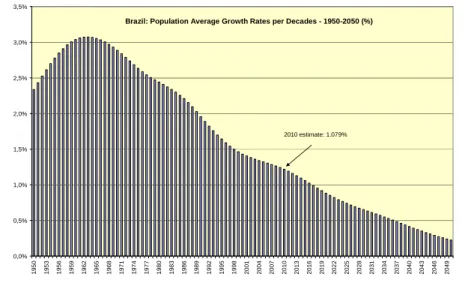
The speed of demographic change in Brazil is also transparent from the following figure, where decadal average population growth rates from 1950 to the present are shown, as well as projections up to 2050. Average ten-year rates peaked in the early 1960s, declined to 1.25% yearly at present (1.079% in 2010) and are expected to reach 0.2% p.a. in 2050.
We conclude that productivity has recovered in the more recent years the ground it had lost in explaining per capita GDP growth. It was helped by demographic changes that
began to work more forcefully in the 1970s and gained momentum since the 1980s. This demographic bonus is a well-known phenomenon in the development literature and is likely to continue in the medium term as more women enter the labor force (thereby increasing the EAP) and the number of people in the relevant working age group continues to grow faster than total population.
Figure 2: Brazil’s Population — 10-Year Average Growth Rates, 1950-2050 (% p.a.)
Brazil: Population Average Growth Rates per Decades - 1950-2050 (%)
0,0% 0,5% 1,0% 1,5% 2,0% 2,5% 3,0% 3,5% 1 9 5 0 1 9 5 3 1 9 5 6 1 9 5 9 1 9 6 2 1 9 6 5 1 9 6 8 1 9 7 1 1 9 7 4 1 9 7 7 1 9 8 0 1 9 8 3 1 9 8 6 1 9 8 9 1 9 9 2 1 9 9 5 1 9 9 8 2 0 0 1 2 0 0 4 2 0 0 7 2 0 1 0 2 0 1 3 2 0 1 6 2 0 1 9 2 0 2 2 2 0 2 5 2 0 2 8 2 0 3 1 2 0 3 4 2 0 3 7 2 0 4 0 2 0 4 3 2 0 4 6 2 0 4 9
2010 estimate: 1.079%
Source: IBGE and IPEADATA
Demographic transition is represented by a reduction in fertility rates, increases in life expectancy rates (longevity) and increased female participation. Its intensity varies with countries and over time but it is commonly associated with urbanization — which is clear in Brazil after the 1940s — and increased female participation in the labor force (EAP), which further contributes to decreases in fertility.13
Thus, total fertility rates fell from 4.02 in 1980 to 2.08 in 2010 (projected) and are not expected to fall much more than that in the future. Life expectancy rose from 62.70 years in 1980 to 70.06 in 2010 (projected) and is expected to climb to 73.59 in 2050. Infant mortality fell from 80.1 per thousands born in 1980 to 28.0 in 2010. The rate is expected to fall even further to 15.1 in 2050. Women accounted for 15% of the labor force in Brazil in 1950, 27% in 1980, 35% in 1989, 41% in 1999 and 44% in 2007.14
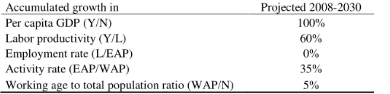
The previous framework can also be used to make projections for the future. This is done in the next table, which contains projections for 2030. Adopting IBGE’s population projections, assuming no change in the rate of unemployment15 and per capita GDP growth
13
Curiously enough, the recently released PNAD results (not included in this version) show a minor increase in fertility in 2009. A survey of the literature on the economic roots of demographic change by Greenwood and Seshandri (2005) examines works that have uncovered a strong empirical nexus between changes in the demographic structure and aggregate macroeconomic variables.
14 Data from the sites www.ibge.gov.br and www.ipeadata.gov.br. Note that these numbers are likely to
change when the 2010 Demographic Census data become available.
15
of 4.5% p.a., labor utilization would account for 40% of total log-average per capita GDP growth, while productivity would be responsible for 60%. The ratio of labor force to the working age population would be the main variable behind increasing labor utilization, as show in the table.16
We conclude that, barring changes in the employment rate — which are not expected to present systematic deviations from present levels in the long run — future growth will depend crucially on the continuation of recent demographic trends, plus productivity change. The former can be taken as exogenous.17 Thus, we should search for the sources of productivity growth as a major theme in investigating GDP growth prospects. Demographic change will not be a hindrance to long term growth in Brazil, due to the demographic transition Brazil that has been experiencing in the past decades, which is likely to continue to deliver a “demographic bonus” to the pace of development in the years to come.
Table 2: Decomposition of Log-Average per capita GDP Growth, 2008-2030 (%)
Accumulated growth in Projected 2008-2030
Per capita GDP (Y/N) 100%
Labor productivity (Y/L) 60%
Employment rate (L/EAP) 0%
Activity rate (EAP/WAP) 35%
Working age to total population ratio (WAP/N) 5% Source: See text.
2.2 Slower growth is correlated with low levels of capital accumulation
Brazil’s growth deceleration, expressed by the collapse of GDP growth after 1980, is associated with the slowdown of capital accumulation. This suggests that we begin our analysis by a decomposition of capital stock growth (K’) into its main components in searching for its major causes. The decomposition proposed next is based on an identity that separates out the effects of: saving rate at current prices (s), capacity utilization (u), capital productivity (v)18 the inverse of the relative price of investment (p) and the rate of depreciation (δ) in explaining capital stock growth:19
K’ = s.u.v.(1/p) – δ
The decomposition results shown below follow a division of periods that has become nearly consensual among Brazil’s economic analysts. It divides the long term into phases characterized by (up to a point) similar performance and economic policy regimes.20
After 1980 growth deceleration characterizes not only GDP but capital stock growth as well, as suggested. During the years of the so-called ‘Brazilian miracle’ of
16
Assuming lower per capita GDP growth decreases the labor productivity share and increases the activity rate share in the decomposition. Thus, assuming 3.5% per capita GDP growth reduces labor productivity’s share to 48% and increases the activity rate’s share to 46%, other things equal.
17
This is a simplification, of course. But linking demographic change and economic growth is beyond the scope of this paper.
18 The productivity of capital is equal to the output-capital ratio adjusted for capacity utilization. 19 This identity is developed in Bacha and Bonelli (2005).
20
The analysis begins in 1947 because Brazil’s National Accounts began to be calculated in that year. The depreciation rate δ is not among the variables in the table because it changed very little between successive
73 capital stock growth reached 9.5% p.a., a rate which increased to 9.7% in the succeeding period — just before collapsing after 1980.21 Slow capital growth, at 2.2-2.3% p.a., prevailed even after stabilization.
As noted by Bacha and Bonelli (2005), it is hard to blame only the saving rate for the collapse after 1980: in fact, it fell approximately only one percentage point of GDP between 1974-80 and 1981-92, from 20.1% to 19.0%. But all the three other components fell much more — in different proportions, though.
Table 3: Decomposition of Capital Stock Growth Rates – Annual Averages in Selected Periods (1948-2009)
Periods K' (% p.a.) s u v (1/p)
1948-62 8.1 0.132 0.977 0.625 1.580
1963-67 6.4 0.141 0.937 0.591 1.396
1968-73 9.5 0.174 0.970 0.583 1.391
1974-80 9.7 0.201 0.966 0.542 1.339
1981-92 3.3 0.190 0.906 0.458 1.023
1993-99 2.2 0.173 0.931 0.442 1.002
2000-09 2.3 0.167 0.947 0.454 0.964
Total 5.8 0.166 0.948 0.528 1.248
Source: Bacha and Bonelli (2010); see text.
From the table results we conclude that the main culprits for slower capital growth after 1980 were reduced capital productivity (v), increased prices of investment (p) and a reduction in capacity utilization (u). This becomes clearer when differences of capital stock growth rates in consecutive periods are analyzed (Table 4).
Thus, for instance, the capital stock growth acceleration from the recession 1963-67 to the ‘miracle’ 1968-73 (+3.1%, from 6.4% to 9.5% p.a.) can be entirely attributable to a 3% absolute change in the saving rate (in fact, fueled by increased foreign savings) plus a 3% absolute change in capacity utilization, given idle capacity in the previous period (as the remaining items actually operated in the opposite direction, restraining capital accumulation).
Table 4: Capital Stock Growth Rates — Differences in Consecutive Periods
Differences K' s u v (1/p)
63/67 - 48/62 -1.7% 0.01 - 0.04 - 0.03 - 0.18
68/73 - 63/67 3.1% 0.03 0.03 - 0.01 - 0.01
74/80 - 68/73 0.2% 0.03 - 0.00 - 0.04 - 0.05
81/92 - 74/80 -6.4% - 0.01 - 0.06 - 0.08 - 0.32
93/99 - 81/92 -1.1% - 0.02 0.02 - 0.02 - 0.02
2000/09 - 93/99 0.1% - 0.01 0.02 0.01 - 0.04
Source: Table 3.
From the ‘miracle’ period to the next one a slight acceleration in K’ was observed (+0.2%), which was entirely due to increased savings (again, foreign-originated). All other
factors contributed to restrain capital accumulation, especially lower capital productivity. Between this last period and the long lost decade of 1981-92 capital stock growth fell from 9.7% to 3.3% p.a., but only a fraction can be attributable to lower savings. All remaining variables displayed highly negative contributions.
Capital accumulation continued to decrease thereafter during the ‘reforms phase’ (1993-99). Blame for this decrease can be shared between a lower rate of savings, a minor reduction in capital productivity and a slight increase in the relative price of investment goods. Finally, in the last period — characterized by a new policy regime from 1999 on — the modest recovery in capital accumulation is explained by higher capacity utilization and, secondarily, by increased capital productivity. The saving rate, in turn, displayed a minor decrease, restraining capital accumulation.
This approach highlights the role of reduced savings in helping to explain capital accumulation, from 20.1% in the phase just before 1980 to 16.7% in 2000-09 — therefore, in accounting for slower economic growth as well, especially as far as future growth is concerned. And this is so because, at present: capacity utilization has reached relatively high levels (thus, one cannot expect much from this source in contributing to increasing capital accumulation); capital productivity tends to increase with fast output growth, but not much (if at all); the relative price of investment goods has fallen because it benefitted from higher capital goods imports, and is approximately stable at present. Therefore, low investment rates (at about 19% of GDP; 2010 estimate), reflecting low savings rates, is the main constraint from the supply side. To this we should add slow productivity growth, a point to which we now turn to.
2.3 Growth Accounting and Total Factor Productivity (TFP)
Without loss of generality we calculated TFP growth as a residual in an aggregate Cobb-Douglas production function with constant returns to scale with neutral technical change. A log linearization of the function yields
Y’ = α.(u.K)’ + (1 – α).L’ + TFP’
where, given the usual hypotheses, Y’ is the output growth rate, α is the income share of
capital, (u.K)’ is the growth rate of utilized capital stock, L’ is the growth rate of employment and TFP’ is TFP’s growth rate.22 The resulting annual series reveal that:23 (a) TFP growth rates display large volatility;24 (b) negative rates are not found very often from the late 1940s to 1980 (just five occurrences: 1952, 1953, 1963, 1975 and 1977); (c) from then on negative TFP rates are not uncommon (for instance: in the 1981-92 years TFP grew only in 1984-86); (d) after 1992 a TFP recovery is observed: TFP only fell five times (usually during recessions).
It is trivial to deduce from the definition of TFP growth that it can be written as a weighted average of capital and labor productivity growth, the weights being α and (1 – α).
This allows for a decomposition of TFP growth into these two components. Table 5 shows
22 The coefficient α was taken as 0.46, its average value for 2000-2007, as the ratio of labor compensation to
total labor compensation plus gross surplus in Brazil’ National Accounts. There is some evidence that this value has been decreasing slightly in recent years.
23
See Appendix 2.
24
the decomposition results in the same time periods shown before, characterized by amply similar origins and consequences of economic policy regimes.
From the table we conclude that Brazil’s productivity performance varied enormously over time. TFP average growth ranged from –1.0% p.a. during the ‘long lost decade’ (1981-92) to 4.0% yearly in the ‘miracle’ years of 1968-73. Note that TFP growth recovered after 1992, but not much. Since 2000 average TFP growth, at 1.0% p.a. until 2009, is more pronounced. Incidentally, the same rate was observed in the long term average.
Table 5: Average TFP Growth Rates Decomposed into Capital and Labor Productivity Contributions, Selected Periods, 1948-2009 (% p.a.)
TFP Due to capital productivity Due to labor productivity
1948-62 2.3% -0.4% 2.7%
1963-67 0.3% -0.7% 1.0%
1968-73 4.0% 0.4% 3.6%
1974-80 1.0% -1.1% 2.0%
1981-92 -1.0% -0.6% -0.4%
1993-99 0.2% -0.1% 0.3%
2000-09 1.0% 0.5% 0.5%
Total (1948-2009) 1.0% -0.3% 1.3%
Source: author’s calculations; see text.
The annual TFP results shown in Table A.2 (Appendix) reveal two interesting aspects. First, the capital productivity contribution to TFP growth is positive only in approximately 1/3 of the years. Usually, years and periods of very fast GDP growth. This also appears in the averages shown in Table 5: the contribution of capital productivity to TFP is positive in two periods, only (1968-73 and 2000-09). Labor productivity growth, on the other hand is negative only rarely: of the 62 rates shown in Table A.2 it is negative in 12 years, all of them characterized by economic recession and loss of output. In terms of period averages, as shown in Table 5, it is negative only during the ‘lost decade’ (1981-92). These findings suggest that productivity is pro-cyclical.
Second, the contribution of labor productivity is always much larger than capital’s, the exception being the average 2000-09, when they are equal. This suggests that labor productivity “sustained” TFP growth in the long term. Considering the 60-odd years average TFP growth of 1.0% (1948-2009), the contribution of labor productivity was 1.3% p.a., while that of capital reached –0.3% per year.
A traditional sources of growth approach is shown next (Table 6), where it is found that capital stock growth accounts for most of GDP growth in most periods — the exception being the most recent phase (2000-09).
Table 6: Sources of Output Growth, Selected Periods, 1948-2009 (%)
GDP TFP % GDP Capital % GDP Labor % GDP
1948-62 7.6% 2.3% 30% 3.9% 51% 1.4% 19%
1963-67 3.5% 0.3% 8% 2.3% 67% 0.9% 25%
1968-73 11.2% 4.0% 36% 4.7% 42% 2.4% 22%
1974-80 7.1% 1.0% 13% 4.3% 61% 1.8% 25%
1981-92 1.4% -1.0% -70% 1.3% 88% 1.2% 82%
1993-99 2.9% 0.2% 6% 1.5% 51% 1.2% 43%
2000-09 3.3% 1.0% 30% 1.0% 32% 1.2% 38%
Total 1948-2009 5.1% 1.0% 20% 2.7% 52% 1.4% 28%
Source: author’s calculations; see text.
The main findings from this section can be summarized as follows: (i) per capita GDP changed mostly in response to productivity growth in the long term; (ii) but the contribution of demographic bonuses in the form of increasing labor utilization has been growing and is likely to continue in the foreseeable future; (iii) slow growth after 1980 followed slower capital accumulation, but savings were only part of the picture; (iv) despite this last conclusion, from now on savings and investment rates must increase for growth to resume; (v) productivity change has recovered, but is needs boosting as well; the record suggests that productivity is pro-cyclical.
In fact, more than one study has identified lack of savings as a major growth constraint in Brazil. According to Hausman, Rodrik and Velasco,25 the poor growth performance can be explained by low saving and too little emphasis on education. The plausibility of the hypothesis rests on observed high returns on capital and education:26 “If domestic savings are scarce, high foreign debt or a large current account deficit would signal that the country is making extensive use of foreign savings… There would also be a strong willingness to remunerate domestic savings through high interest rates… The challenge for Brazil is to explain why domestic savings do not rise to exploit large returns to investment (Hausman, Rodrik and Velasco, 2005).”
The answer, as suggested by the authors, lies in issues to be explored in the next section: “Brazil … suffers from an inadequate business environment, a low supply of infrastructure, high taxes, high prices for public services, weak contract enforcement and property rights, and inadequate education… Investment is … constrained by the country's inability to mobilize enough domestic and foreign savings (not anymore, apparently; our addition) to finance investment at reasonable rates… A more sustained relaxation of the constraint on growth would therefore involve increasing the domestic savings rate… Brazil's share of public revenue, at 34 percent of GDP, is by far the highest in Latin America and one of the highest in the developing world. Yet public savings have been negative … High taxes and low savings reflect high spending and social transfers and
25
The growth diagnostics approach created by Hausman, Rodrik and Velasco (2005) has been used to analyze growth barriers in Brazil in, for instance, Bonelli and Pinheiro (2008) and Blyde et al. (2010).
reduce the disposable income available to the formal private sector...” (Hausman, Rodrik and Velasco, 2005, passim)27
One of the main conclusion from their analysis is that a lower tax burden resulting from lower public expenditures would contribute both directly to increased savings (because it would allow the public sector to save) and indirectly (by increasing funds available to the private sector).
The list of issues just cited suggests the approach to be adopted next in order to deepen the analysis on growth barriers, when we turn to factors that have inhibited savings, investment and productivity. The analysis focuses on five main issues: high tax burden, weak institutional pillars, insufficient infrastructure, inadequate finance, and low educational levels. Thus growth-enhancing reforms should focus on improving: (i) the fiscal stance; (ii) institutions and related policies (especially through regulatory reform); (iii) infrastructure (implying increased public expenditures, which require shifts in the structure of expenditures); (iv) financial development (which presumes a larger role for private agents, opposing the recent trend towards increasing the state presence in granting long and short term loans); and (v) human capital.
3. Obstacles to Growth Acceleration
The list of factors deemed responsible for the country’s less-than-expected growth is large and covers a broad array of subjects, as noted. In what follows a reasonably common set of explanatory factors is analysed, following the suggestions at the end of the previous section. The next section takes up the theme of reform proposals and discusses policy alternatives.
3.1 The obstacle represented by a high tax burden
The obstacle to growth represented by a high tax burden has been clearly recognized in the literature. In Brazil, the rise in public current spending that underlies increases in the tax burden has among its roots the new obligations in the 1988 Constitution (or immediately thereafter), when a phase of 20 years of fiscal centralism ended and a large share of tax revenues was transferred to sub-national governments (state and municipalities), but without a corresponding reallocation of responsibilities. While state and municipal governments used revenue windfalls to increase consumption and hire civil servants, the federal government contracted non-discretionary spending (mostly investment) and attempted to decentralize responsibilities. Eventually, the federal government transferred most activities in health, education and public transportation to the states and municipalities, but remained responsible for financing some of them (in health, for instance). The 1988 Constitution and other reforms also expanded social security expenditures and created more generous retirement rules for civil servants and private sector workers, notably in the rural sector.
In the initial years after its enactment, the central government financed its growing current expenditures counting on an inverse Tanzi effect (since revenues were better indexed to inflation than expenditures) and on augmented seignorage revenues. When
27
inflation was tamed (after 1994), the government relied on expanding the public debt. High interest rates on government bonds have kept their attractiveness, but are costly as far as GDP growth is concerned, for they set a floor to all other interest rates in the economy. They also contribute to increase overall government’s expenditures.28
Increased borrowing was accompanied by raising taxes. The federal government, in particular, boosted its tax proceeds by creating new taxes and raising rates on social contributions,29 with three important effects: (i) they counterbalanced decentralization promoted by the Constitution and, indeed, brought about some re-centralization; (ii) the quality of the tax system worsened; and (iii) as no compensating tax reduction occurred in states and municipalities, the total tax burden increased.30
The surge in public consumption (primary expenditures, which include retirement, pensions, etc.) was so large that, notwithstanding the rise in debt and taxes, it could only be accommodated due to a significant decline in public investment: summing the public administration and federal SOEs, public investment dropped from 7.9% of GDP in 1968-78 to 2.7% of GDP in 2003-05.31
Infrastructure was especially hit, with public investment in this area (including SOEs) declining by about 4% of GDP between 1971-80 and 2001-03, a contraction that was not at all compensated by a rise in private infrastructure spending. One of the consequences has been the deterioration in physical infrastructure, with negative effects on productivity growth. As a late recognition of this fact, investment in infrastructure has recently been elected a top priority in the government agenda, as witnessed by the
launching of PAC — Programa de Aceleração do Crescimento (Growth Acceleration
Program) in early 2007. Infrastructure spending accelerated since then, but: results are slow to appear; and the level of spending is still below what is needed.
To evaluate the impact of taxation increases and simultaneous infrastructure investment reductions on Brazil’s long-term growth Pinheiro, Bonelli and Pessôa (2009) developed a counterfactual exercise that simulated what would have happened to Brazil’s long-term growth had taxation and infrastructure investment stayed at levels similar to those observed before the 1988 Constitution was enacted. They found that the adoption of this course of action led to a 2006 GDP level 18% smaller when compared to the counterfactual scenario. Such accumulated GDP reduction, spread through nearly 20 years, amounts to an annual average decrease of almost 1 percentage point in the growth rate of GDP. The increase in the tax burden was identified by the authors as a ‘reform’ that took
28
Public consumption increased from an average of 10.9% of GDP in 1951-80 to 20.0% in 1995-2005, while both public savings and investment fell substantially. (Pinheiro, Bonelli and Pessôa, 2009) The share of public consumption on GDP has been kept after approximately at 20% since 2005 (includes investment and current expenditures on goods and services; source - Quarterly GDP database, IBGE).
29
A ‘contribution’ is a kind of tax that is not shared with sub national governments.
30 The number of tributes increased as well. Some of them are applied cumulatively, some share the same tax
base and others have rates that vary with time and region of the country. The final result is a complex, unstable and costly tax system. Among other things, this complex system has increased investment risk and fostered informality, with negative consequences for human capital investment and productivity growth (Pinheiro, Bonelli and Pessôa, 2009).
the economy away from the kind of market-based economic model aimed at when adopting privatization, trade and financial liberalization and de-regulation.32
Thus, the importance of a disproportionately high tax burden is a crucial factor in explaining low savings and investment rates. In addition, the next table shows that Brazil’s tax burden is not only high compared to developing countries such as Mexico and Turkey, but has been increasing substantially as well.33 In 2008 it was only slightly lower than OECD’s average (34.4% compared to 35.1%) and much higher than the average in Latin America.34
Note that the temporary fall observed in 2009 was due to the fiscal policies adopted to deal with the domestic recession after the 2008 world crisis — mainly, reduction of taxes on consumer durables (cars, furniture, and electric and electronic appliances, mostly), capital goods and construction material — and to the recession itself. Parts of these incentives to boost spending were discontinued in the second quarter of 2010.
Table 7: Tax Burden—Brazil (2000-10) and selected OECD countries (2008) (% of GDP)
2000 29.98 Japan 17.6
2001 30.89 Mexico 20.4
2002 32.01 Turkey 23.5
2003 31.5 United States 26.9
2004 32.31 Ireland 28.3
2005 33.38 Switzerland 29.4
2006 33.35 Canada 32.2
2007 33.95 Spain 33
2008 34.41 New Zealand 34.5
2009 33.58 United Kingdom 35.7
2010 34.6 Germany 35.4
Brazil’s increase 2000-10 in p.p. 4.6 OECD average (all countries) 35.1 Sources: Receita Federal do Brasil and OECD; Brazil’s estimate for 2010 is preliminary.
Pres. Lula’s second term (2007-10) has been characterized by increased government expenditures. The trend was reinforced after the 2008 crisis, as the federal government augmented spending as an action to counterbalance the crisis effects. In addition to that, a strong fiscal impulse has also been based on large real minimum wage increases.35
This state of affairs has continued even after it became clear that Brazil had experienced only a short recession in late 2008-early 2009. The government has resorted to the justification that policies of increased expenditures have been adopted nearly
32
Three additional problems associated with Brazil’s high tax burden are: (i) the uncertainty brought about by a high public debt to GDP ratio, which contributes to high interest rates; (ii) the rigidity of the main budget expenditure items, which include many earmarking provisions that allow the authorities very little discretion and make fiscal policy pro-cyclical; and (iii) the complexity of the tax structure, which imposes a further burden on economic agents. (Pinheiro, Bonelli and Pessôa, 2009, passim)
33 The increase from the pre-Constitution years to the late 2000s amounts to nearly 12% p.p. of GDP. In
2005-09 approximately 70% of the tax burden was due to federal taxes and ‘contributions’, 26% to states’ and 4% to municipalities’.
34
18.4% of regional GDP, according to ECLAC (2010).
35
everywhere. As a result, the presence of the State in the economic sphere has been greatly enhanced. This aspect has implications for the process of institutional development as well.
In addition, in 2010 a worsening of the fiscal position is expected. At the same time ‘creative’ use of Treasury lending to the National Development Bank (BNDES) has succeeded in keeping the net public debt approximately constant, while the gross debt increases.36
3.2 Institutional or policy settings that could explain past performance
The quality of institutions has been recognized as a key factor in economic development. But institutional development takes place slowly, its impact on growth is not easy to gauge when time series information for individual countries are used to evaluate it, and there is no clear answer as to which institutions are more important to enhance growth. A related controversial issue is causality, because institutions are simultaneously cause and consequence of growth.37
Therefore, analyses and conclusions from individual countries over short time spans should be viewed with a grain of salt, or as merely indicative. The least that can be said is that the creation and working of clear and respected regulatory frameworks and strict observance of the rule of law are important as sources of growth due to their allocative effects on factor use and aggregate supply. This is one of the instances in which it seems safe to say that institutional reform antecedes growth.
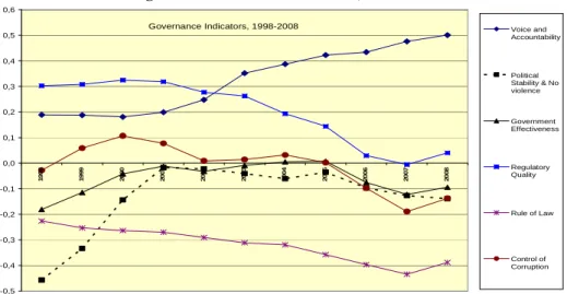
In what follows we use a World Bank database — namely, the World Governance Indicators (WGI)38 — to evaluate Brazil’s institutional development according to the six dimensions covered by the WGI survey: (i) Voice and Accountability; (ii) Political Stability and Absence of violence; (iii) Government Effectiveness; (iv) Regulatory Quality; (v) Rule of Law; (vi) Control of Corruption. We compiled series of 3-year moving averages for these indicators, which are shown in the next figure.39
The main conclusion from the figure is straightforward: over the decade analyzed Brazil has improved its position relative to the world average in one dimension only: Voice and Accountability.40 This is one of the two dimensions in which Brazil has displayed above world average grades during the whole period for which the indicator is available.
36
The accounting procedure is such that the lending is backed by assets (loans extended by the by BNDES) that presumably will be paid out in due time.
37
Besides, if, on the one hand, institutional reform can be facilitated during a growth phase, on the other existing growth may imply that reforms are not necessary, because growth has been occurring without their help.
38
See Kaufmann, Kraay and Mastruzzi (2009), or KKM, for short. The governance indicators are measured in normalized units ranging from -2.5 to +2.5 (the world average is zero), with higher values corresponding to better governance outcomes. They cover 212 countries and territories and include hundreds of variables from 35 different data sources to capture the views of tens of thousands of survey respondents worldwide, as well as thousands of experts in the institutes, think tanks, NGOs and international organizations both in the private and public sectors on the quality of governance.
39 The indicators are available for the years 1996, 1998, 2000 and from 2002 to 2008 on a yearly basis. We
added averages for 1997, 1999 and 2001 to fill the gaps and allow for the construction of 3-year averages for the decade beginning in 1998 and ending in 2008. The 2009 dataset is not available yet.
40
Indeed, the country has been steadily improving its position over time, at least until 2008 (average 2006-08).
The other dimension in which Brazil has been performing above world average is regulatory quality: “the ability of the government to provide sound policies and regulations that enable and promote private sector development.” (KKM, 2009) In this case, however, the record shows a peak in 2000 and a gradual worsening over time up to 2007, with a recovery in 2008. With few exceptions, the capture of regulatory agencies in the more recent years by specific interest groups (with close links with the sector ministries they are expected to regulate) has implied a worsening in this dimension, as future research will probably show. In a sense, this is also reflected in the “control of corruption” dimension (next).
Figure 3: Governance Indicators, 1998-2008
Governance Indicators, 1998-2008
-0,5 -0,4 -0,3 -0,2 -0,1 0,0 0,1 0,2 0,3 0,4 0,5 0,6 1 9 9 8 1 9 9 9 2 0 0 0 2 0 0 1 2 0 0 2 2 0 0 3 2 0 0 4 2 0 0 5 2 0 0 6 2 0 0 7 2 0 0 8 Voice and Accountability Political Stability & No violence Government Effectiveness Regulatory Quality Rule of Law Control of Corruption
Source: Kaufmann, Kraay and Mastruzzi; see text
The control of corruption dimension — “the extent to which public power is exercised for private gain, including both petty and grand forms of corruption, as well as elite ‘capture’ of the state” (KKM, 2009) — represents a case in which progress in the initial years, up to 2000, was compromised afterwards. After remaining at world average levels until 2005, the indicator drops until 2007 and recovers a little in 2008.
Brazil’s record in all other three dimensions has been, and still is, poor relative to the world average. Furthermore, the trends over time not always point to positive achievements: (i) government effectiveness (“the quality of public services, the capacity of the civil service and its independence from political pressures; the quality of policy formulation”) improved until 2005 — only to drop afterwards; (ii) political stability and absence of violence (“the likelihood that the government will be destabilized by unconstitutional or violent means, including terrorism”) improved until the early 2000s, but fell a little afterwards;41 (iii) and the rule of law dimension (“the extent to which agents
41
have confidence in and abide by the rules of society, including the quality of property rights, the police, and the courts, as well as the risk of crime”) has always been the dimension characterized by the lowest record — and one in which the curve in the figure above shows a constant decline until 2007.
The conclusion is that Brazil’s record in terms of institutional quality has not been brilliant relative to the world average. The average for all six indicators is exactly the same in 1996 and in 2007. There was improvement in 2008, though. But there is a long way to go before governance levels and institutional quality become similar to those found in most advanced economies. And it is feared that the process of ‘capture’ of regulatory agencies by interest groups and politicians that has been going on since Pres. Lula’s first term will hardly be reflected in institutional improvements.42
In a previous work (Bonelli, 2009) the analysis of the WGI dataset for 2006 allowed for the following conclusions: (i) all six dimensions are highly correlated, the highest correlation coefficient being the one between regulatory quality and government effectiveness (R = 0,95); (ii) cross country regression equations (including 175 countries) for each dimension against per capita national income result in positive associations and show that Brazil was below the average — meaning that its record was that of a country with a higher income — in only one dimension: political stability and freedom of expression. In all the other ones the Brazilian indicator was characteristic of a country with lower per capita income than the actual one.
Repeating the exercise with the WGI 2008 dataset yields essentially the same results, but now: (i) the highest correlation occurs between “corruption” and the “rule of law” dimensions (R=0.947), followed by the one between “government effectiveness” and “rule of law” (R=0.934); (ii) “government effectiveness” and “regulatory quality” are also closely related (R=0.932).
More recent data from the Global Competitiveness Report (GCR) 2010-2011 (World Economic Forum, 2010) shows that Brazil lost in 2010 little of the ground it had acquired in the previous years: the Report’s latest issue shows that Brazil went from the 56th to the 58th position among 139 countries between 2009 and 2010. It ranks especially low in the pillars related to “Goods Market Efficiency” (114th), “Macroeconomic Environment” (111th), “Labor Market Efficiency” (94th), “Institutions” (93rd), and “Health and Primary Education” (87th);43 and less so in “Financial Market Development” (50th), “Technological Readiness” (54th) and “Infrastructure (62nd).44 In particular, the Report estimates that investment in infrastructure should reach (at least) 5 percent of GDP to keep infrastructure from becoming a bottleneck to achieving sustained (high) growth rates in the future.
Thus, the institutional environment remains relatively weak in areas related to legal and regulatory issues, a situation that tends to deteriorate with the on-going process of
42
Few agencies are truly independent at present. Most have either become inoperative or subject to the ministries whose activities they are supposed to regulate.
43 Note that the median is 69.5.
44 On the positive side the GCR 2010-2011 also notes that “Brazil displays one of the most developed and
capture of firms and agencies by particular interests, and contract enforcement. The country’s business environment is also dragged down by a high cost of doing business, and less-developed human capital. On the other hand, a high degree of IPO activity contributes to the country’s relatively high scores in non-banking financial services, according to the GCR 2010-11.
The high cost of doing business in Brazil has also been measured by the country’s position in international comparisons. The latest World Bank Doing Business 2010 report has ranked Brazil in the 129th position among 183 countries. What is worse, Brazil lost two positions from the previous report, indicating that excessive regulation and bureaucratic procedures have not been solved or, at least, dealt with.45
From the report we conclude that private investment presently faces three key challenges to improving business environment conditions: (i) regulatory bottlenecks and political uncertainties; (ii) excessive renegotiations of concessions; and (iii) the lack of efficiency of regulatory agencies, a process which has been worsening in the recent past. The coincidence of analyses in the GCR and the Doing Business reports with the WGI indicators is suggestive of the weakest institutional aspects, or dimensions. It is also fitting to bring attention to the fact that juridical uncertainty is associated with fragile legal and regulatory frameworks. All these dimensions tend to constrain investment and growth.
3.3 Impediments to investment in infrastructure
Its has long been established that the availability and quality of infrastructure services of telecommunications, road and railroad transportation, ports, transmission and distribution of energy, and water and sanitation lead to higher productivity and lower costs for the private sector, thereby facilitating growth and increasing its prospects. Accordingly, many empirical studies that have examined the relationship between infrastructure investment and economic growth have found a positive and significant association between the two (Rozas, 2010).46 Studies have also found a correlation between infrastructure investment and overall investment.47
To what extent is infrastructure a binding constraint to growth in Brazil? It is a known fact that the growth slowdown in Brazil occurred simultaneously with the reduction of expenditures in infrastructure. The reduction in infrastructure investment reflected the retrenchment in public investment, including both central and local governments and state enterprises. Privatization and regulatory reform have not been able to reverse this decline (Blyde et al., 2010). Bur a recent study has found that central government infrastructure investment has recovered steadily since 2003: having reached only 0.31% of GDP in that
45
Thus, for instance, the Brazil time spent on paying taxes is the highest in the world: 2,600 hours per year (World Bank, 2009, p. 58). Reforms in 2008-09 have been more effective in the procedures related to starting businesses (ibid, p.98).
46
A pioneering work for Brazil has found that the causation runs from infrastructure investment to growth (Ferreira and Maliagros, 1998).
47 In the case of Brazil the following conclusion holds, as shown by Ferreira and Araujo (2007): “Having
year, the ratio went to 1.02% in 2009 and is estimated to reach 1.14% in 2010. During Pres. Cardoso’s term this ratio had averaged 0.83% of GDP.48
In fact, the issue is common to many countries. Part of the growth slowdown in Latin America, for instance, has been attributed to lower infrastructure investment.49 The reduction of capital expenditures, a general phenomenon in the region, is characteristic of the times of fiscal restrictions, when public investments were curtailed. A good part of the burden of fiscal adjustment was felt first and with more intensity in infrastructure. Many studies also found that there is a correlation between increased public sector deficits and reduced public investment infrastructure expenditures made by the public sector, a situation that began in the early 1980s as the foreign debt crisis erupted. Not coincidentally, at that time Brazil (and other countries) started its growth collapse. The need to have fiscal adjustment together with servicing an increasingly costly external debt led countries to restrain public expenditures, mostly on capital investment. The same continued to occur in the 1990s, as the fiscal crises in many states forced them to postpone infrastructure expenditures before sacrificing consumption and debt service expenditures.50
Thus, the annual average of infrastructure investment in the main economies in Latin America during 1980-1985, 1996-2001 and 2002-2006 went from 3.7% of GDP to 2.2% and to 1.5% (Rozas, 2010). Ferreira and Gonçalves do Nascimento (2005) estimate that the decline in public investment since the early 1980s, largely concentrated on infrastructure, lowered Brazil’s annual GDP growth by about 0.4 percentage points.
As mentioned, the public investment decline in Brazil has also been due to the effort to generate budget surpluses, as in the other countries of Latin America. One political explanation for the myopic behavior of policy makers, who restrain infrastructure investment in order to solve fiscal constraints, is that “with short-term tenures (e.g., four or six years) they have little incentive to consider the future gains of infrastructure expenditures.” (Ferreira and Araujo, 2005)
Another explanation lies in one crucial characteristic of Brazil’s recently adopted policy mix: its reliance on private and public consumption as growth-enhancing variables, even before the 2008 crisis.
Thus, infrastructure spending in Brazil declined from the 1970s to the early 2000s. It averaged 5.4% of GDP during the 1970s, 3.6% in the 1980s, 2.3% in the 1990s, and 2.1% in the 2000s, and has been identified as one of the binding constraints in the near future, despite recent efforts by the central government: “Although part of the decline in SOE investment stems from changes in classification, as a result of privatization, the bulk of it had already happened by 1990-94, before the peak of privatization in 1996-98. Indeed, the decline in public investment is underestimated, for it does not take into account the contraction in investment by state and municipal SOEs. The main consequence of this fall in public investment has been the deterioration in the quantity and quality of infrastructure.” (Blyde et al., 2010)
48 See O VALOR, November 8, 2010, p. A5.
49 Calderon and Serven (2003) estimated that one third of the growth difference between Latin America and
East Asia is due to underinvestment in infrastructure.
50
Macroeconomic instability contributed to the observed decline until recently, as it increased the cost of capital and implied uncertainty towards the future.51 According to the World Bank (2007, p. 25), however, although “evidence shows that higher infrastructure investments may lead to higher growth rates and better social indicators … it is not possible to claim that infrastructure is a binding constraint to higher sustainable growth rates in Brazil — especially when compared to high current expenditures and high levels and incidence of taxation”. This is not to say, of course, that it may not become a binding constraint, if infrastructure investment stays at their current low levels.
Frischtak (2007) estimates that public and private investment in infrastructure has averaged only 2.21% of GDP in 2001-2006 (water and sanitation, electric energy, communications and road construction account for 93% of the total, railroads, airports, ports, hydro ways for 7%). He notes the central role played by BNDES, the National Development Bank, in accounting for these results: “In 2007 investment in infrastructure reached R$ 57.3 billion (2.15% of GDP), of which 12.4 by the central government and 44.9 by private and public enterprises. Of these, BNDES disbursements came to represent 53.5%.” (Frischtak, 2007)
A recent mapping of infrastructure projects at the sector level, planned for the present and for the next three years put infrastructure investment at R$274 billion in 2010– 13, or 37% higher than the R$199 billion disbursed in 2005–08. The estimate for 2010–13 corresponds to only 2.2% of GDP — in line with the average 2.1% of GDP spent in recent years (Borça and Quaresma, 2010).
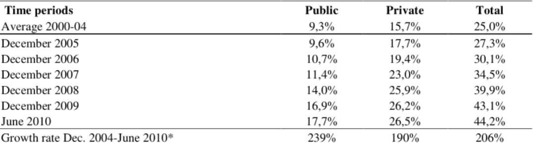
Over the past 10 years, the private sector has accounted for almost 90% of total investment (not only infrastructure) in Brazil, while the public sector was responsible for the remaining 10% (ibid). In infrastructure investment, however, the private and public sectors have shared the burden. The bulk of total projected infrastructure investment in 2010-13 is concentrated in the electricity sector, which is expected to account for about
one-third of total infrastructure investments during the next four years.
Telecommunications come second, with a share of 24.5% of the total, followed by water and sewage with a share of 14.2%.
Thus, public sector investment in infrastructure, albeit increasing, has been low. It could grow even more over time if authorities manage to create enough fiscal space. A crucial challenge to increasing public sector investment in infrastructure without reducing consumption expenditures is that the tax burden is already high. In addition, most of the budget is earmarked for hard-to-curb expenditures like payroll and social security. As to challenges to the private sector, the main ones are the legal and regulatory frameworks, as mentioned above.
3.4 Financial Development
Financial development is usually measured by factors such as size, depth, access, efficiency and stability of a given financial system. Evidence suggests that both the level of banking sector development and stock market development exert a causal impact on economic growth (and are highly correlated with subsequent GDP per capita growth as
51